Structure Factor of a Relaxor Ferroelectric

Abstract

We study a minimal model for a relaxor ferroelectric including dipolar interactions, and short-range harmonic and anharmonic forces for the critical modes as in the theory of pure ferroelectrics together with quenched disorder coupled linearly to the critical modes. We present the simplest approximate solution of the model necessary to obtain the principal features of the correlation functions. Specifically, we calculate and compare the structure factor measured by neutron scattering in different characteristic regimes of temperature in the relaxor PbMg_1/3Nb_2/3O₃.

I Introduction

Relaxor ferroelectrics, a typical example of which is PbMg_1/3Nb_2/3O₃ (PMN), a perovskite in which the Mg²⁺ and Nb⁵⁺ randomly occupy the octahedrally coordinated site, have a very high dielectric constant for a very wide region in temperature and have no ferroelectric transition except in applied electric fields. Cowley et al. Cowley2011a in a detailed review of relaxor ferroelectrics have commented that although they were first synthesized over 50 years ago and their properties have been well explored, a satisfactory theory explaining their properties has not yet been formulated. Here, we present a minimal model for the canonical relaxor PMN and its simplest necessary approximate solution based on Onsager’s results on models with dipolar interactions, the displacive transition model of pure ferroelectrics, and quenched random fields.

The properties of the relaxors such as PMN may be summarized as follows: Cowley2011a ; Bokov2006a ; Kleeman2006a ; Samara2003a ; Cross1987a in zero external electric field they have a region of collective dielectric fluctuations which is bounded at the upper end by a temperature $T_{B}$, the Burns temperature, Burns1983 above which the susceptibility has a Curie-Weiss form. Viehland1992a A broad region extending down to $T=0$ below $T_{B}$ is marked by a temperature $T_{\max}$ where the susceptibility is maximum and has a width in temperature $\Delta T_{\max}$. Both $T_{\max}$ and $\Delta T_{\max}$ depend on the frequency $\omega$ at which the dielectric susceptibility is measured. Smolenskii1970a ; Bovtun2004a ; Hlinka2006a ; Bokov2012a ; Glazounov1998a Very significantly, neutron scattering experiments have revealed that the structure factor $S_{\bm{q}}$ has unusual temperature Gvasaliya2005a ; Hiraka2004a ; Gehring2009a , power-law Gvasaliya2005a forms and anisotropies, Xu2011a which are unlike those in the random field or the random bond disorder models with short-range interactions. Imry1975a ; Blinc1999a ; Westphal1992a

Typically only such interaction models with quenched disorder have been used to describe relaxor ferroelectrics. These models in three dimensions for weak disorder also have long-range order at a finite temperature, Imry1975a which is not observed in the canonical relaxor PMN. Cowley2011a Several other models have been proposed for relaxors, Glinchuk2004a ; Burton2006a ; Tinte2006a ; Akbarzadeh2012a ; Takenaka2013a ; Sherrington2014a - including those of Burton et al. Burton2006a and of Tinte et al. Tinte2006a which just like it is done in the present paper, considers well-known effective Hamiltonians for conventional ferroelectrics with quenched disorder - however, they have almost exclusively been solved by numerical methods, which makes it difficult to determine general aspects of the solution of such models.

Recently, it has been proposed that the ground state of relaxors is that of a cluster glass in which polar domains generated by random fields cluster at low temperatures due to frustrating nature of the dipolar force. Kleemann2014a The mechanism by which such a glassy state is formed is described by the subsequent formation of polar domains due to random electric fields and the clustering of mesoscopic domains due to frustrated random dipolar interactions. While we do not study this problem here, we cannot rule out that such freezing mechanisms may be out of reach of the theoretical treatment that is presented here, as nucleation of polar domains within the disordered matrix may occur as there are stable ordered states in the free energy of our model. Guzman2013a Such domains would then interact through the dipolar force, which is in itself frustrating due to its anisotropy.

In a previous paper, Guzman2013a we developed a variational method which allowed us to study the temperature evolution of the free energy with compositional disorder, which is essential to understand the dielectric properties of solid solutions of relaxors with conventional ferroelectrics such as PbMg_1/3Nb_2/3O₃-PbTiO₃ (PMN-PT). We found that there are disordered states with a region of metastability that extends to zero temperature for moderate disorder and that field-induced transitions to stable ferroelectric states can occur only for applied electric fields sufficiently large to overcome the energy barriers that result from disorder. Here, we present a different solution of the model based on Onsager’s results on systems with dipolar interactions Onsager1936a that provides an important physical insight that is not obvious from the variational solution.

In formulating the minimum necessary model for PMN, it is important to recall Onsager’s result Onsager1936a that unlike in the Clausius-Mossotti or Lorentz approximation, dipole interactions alone do not lead to ferroelectic order except at $T=0$. Moreover, pure ferroelectric transitions were understood with the realization Cochran-Anderson that they are soft transverse optic mode transitions due to dipoles induced by structural transitions so the low temperature phase does not have a center of symmetry. The first point is not in practice important for pure ferroelectrics which are well described by a mean-field theory for the dielectric constant, and is often a first order transition only below which the dipoles are produced. Lines1977a But as we show below, in the relaxor PMN the random location of defects acts in concert with the dipole interactions to extend the region of fluctuations to zero temperatures. Therefore dipole interactions must be a necessary part of the model. The essential physical points in the simplest necessary solution is to formulate a theory which considers thermal and quantum fluctuations at least at the level of the Onsager approximation Onsager1936a and random field fluctuations at least at the level of a replica theory. DeDominicis_book

II Model Hamiltonian

We consider the model Hamiltonian presented in Ref. [Guzman2013a, ], which we present here for the sake of completeness. We focus on the relevant transverse optic mode configuration coordinate $u_{i}$ of the ions in the unit cell $i$ along the polar axis (chosen to be the $z$-axis). $u_{i}$ experiences a local random field $h_{i}$ with probability $P(\{h_{i}\})$ due to the compositional disorder introduced by the different ionic radii and different valencies of Mg⁺², Nb⁺⁵ in PMN. The model Hamiltonian is

$$H =\sum_{i}\left[\frac{\Pi_{i}^{2}}{2M}+V(u_{i})\right]-\frac{1}{2}\sum_{i,j}v_{ij}u_{i}u_{j}$$

$$~{}~{}~{}~{}~{}~{}~{}~{}~{}~{}~{}~{}~{}~{}~{}~{}~{}~{}~{}~{}~{}~{}~{}~{}~{}~{}~{}~{}~{}~{}~{}~{}-\sum_{i}E_{i}^{ext}u_{i}-\sum_{i}h_{i}u_{i},$$ (1)

where $\Pi_{i}$ is the momentum conjugate to $u_{i}$, $M$ is an effective mass and we have included an external electric field $E_{i}^{ext}=E_{0}^{ext}+E_{i}^{ext}(t)$, with a static and uniform component $E_{0}^{ext}$ and an infinitesimally small time-dependent component, $E_{i}^{ext}(t)$. We assume the $h_{i}$’s are independent random variables with zero mean and variance $\Delta^{2}$. $V(u_{i})$ is an anharmonic potential,

$$V(u_{i})=\frac{\kappa}{2}u_{i}^{2}+\frac{\gamma}{4}u_{i}^{4},$$ (2)

where $\kappa,~{}\gamma$ are positive constants. $v_{ij}$ is the dipole interaction,

$$v_{ij}/{e^{*}}^{2}=\begin{cases}3\frac{(Z_{i}-Z_{j})^{2}}{|{\bm{R}}_{i}-{\bm{R}}_{j}|^{5}}-\frac{1}{|{\bm{R}}_{i}-{\bm{R}}_{j}|^{3}},&{\bm{R}}_{i}\neq{\bm{R}}_{j}\\ 0,&{\bm{R}}_{i}={\bm{R}}_{j},\end{cases}$$ (3)

where $e^{*}$ is the Born effective charge and $Z_{i}$ is the $z$-component of ${\bm{R}}_{i}$. The Fourier transform of the dipole interaction $v_{\bm{q}}/(n{e^{*}}^{2})=1/(n{e^{*}}^{2})\sum_{i,j}v_{ij}e^{i{\bm{q}}\cdot({\bm{R}}_{i}-{\bm{R}}_{j})}=\frac{4\pi}{3}\left(1-3\frac{q_{z}^{2}}{|{\bm{q}}|^{2}}\right)-\zeta|{\bm{q}}a|^{2}+3\zeta(q_{z}a)^{2}$ is non-analytic for ${\bm{q}}\to 0$. For future use, we denote $v_{0}^{\perp}=4\pi n{e^{*}}^{2}/3$ as the ${\bm{q}}\to 0$ component of $v_{\bm{q}}$ in the direction transverse to the polar axis (${\bm{q}}\perp\hat{\bm{z}})$, $n$ as the number of unit cells per unit volume, and $a$ as the lattice constant. $\zeta$ is a dimensionless coefficient that depends on the structure of the lattice. Aharony1973a

The Hamiltonian of Eq. (II) presents (i) long ranged (anisotropic) dipolar interactions; (ii) compositional disorder; and (iii) anharmonicity. We now present the procedure used to find the correlation functions for (II). We use the quasi-harmonic approximation, similar to that used for pure displacive ferroelectrics to treat anharmonicity. Lines1977a This reduces the problem to that of harmonic oscillators with a renormalized stiffness which is determined self-consistently. Disorder is treated by an approach which may be termed the “poor man’s replica method”, and has been used to study two and three dimensional magnets with quenched random fields. Vilfan1985a The Onsager approximation, which may be considered the leading fluctuation correction over the mean-field approximation VanVleck1937a is used for the dipolar interactions as well as for the general statistical-mechanical treatment of the problem.

III Solution by Onsager Cavity Method

In this approximation,

$$H \approx \sum_{i}H_{i}=\sum_{i}\left(H_{i}^{0}-h_{i}u_{i}-E_{i}^{cavity}u_{i}\right),$$ (4)

with $H_{i}^{0}=\Pi_{i}^{2}/(2M)+V(u_{i})-(\lambda/2)u_{i}^{2}$. $E_{i}^{cavity}$ is the Onsager cavity field,

$$E_{i}^{cavity}=\sum_{j}v_{ij}\left<u_{j}\right>-\lambda\left<u_{i}\right>+E_{i}^{ext}.$$ (5)

$\left<X\right>$ denotes the thermal average of any quantity $X$; similarly we will denote by $\overline{\left<X\right>}$, the configurational average over the quenched random fields $h_{i}$ taken after the thermal average is taken.

Onsager calculated the parameter $\lambda$ for the simpler problem of dipolar forces alone using continuum electrostatics. More generally, one may determine $\lambda$ by use of a self-consistent procedure such that the response functions obey the fluctuation dissipation theorem. Brout1967a To find the self-consistent response functions, we consider the thermal average of $u_{i}$ made up of a static and uniform order-parameter $p=\overline{\left<u_{i}\right>}$ and a linear response part $\delta\left<u_{i}\right>$, i.e., $\left<u_{i}\right>=p+\delta\left<u_{i}\right>$. The linear response is determined from the cavity field $E_{i}^{cavity}$, Lines1977a

$$\delta\left<u_{i}\right>=\phi_{h_{i}}(\omega)\delta E_{i}^{cavity},$$ (6)

where $\phi_{h_{i}}(\omega)$ is the dielectric susceptibility for the problem with Hamiltonian, $H_{i}^{0}-u_{i}h_{i}-u_{i}p(v_{0}^{\perp}-\lambda)-u_{i}E_{0}$ and $\delta E_{i}^{cavity}=\sum_{j}v_{ij}\delta\left<u_{j}\right>-\lambda\delta\left<u_{i}\right>+\delta E_{i}^{ext}(t)$. To take the average over configurations, we assume that the effects of the random fields $h_{i}$ decouple in $\phi_{h_{i}}(\omega)$ and $\left<u_{i}\right>$. For our model, as will be shown below, $\overline{\phi_{h_{i}}}(\omega)$ is independent of $i$ and therefore has only a ${\bm{q}}=0$ component denoted simply by $\overline{\phi_{h}}(\omega)$. Then taking a Fourier transform, we get the formal expression for the susceptibility function,

$$\chi_{\bm{q}}(\omega)=\frac{\overline{\delta\left<u_{\bm{q}}\right>}}{\delta E_{\bm{q}}^{ext}}=\frac{\overline{\phi_{h}}(\omega)}{1+\overline{\phi_{h}}(\omega)\left(v_{\bm{q}}-\lambda\right)}$$ (7)

Next we determine $\phi_{h}(\omega)$. The equation of motion for $u_{i}$ due to $H_{0}-h_{i}u_{i}-u_{i}p(v_{0}^{\perp}-\lambda)-u_{i}E_{0}^{ext}$ and including a damping force characterized by $\Gamma$ are

$$M\ddot{u}_{i} =-\frac{dV(u_{i})}{du_{i}}+\lambda u_{i}+h_{i}+p(v_{0}^{\perp}-\lambda)$$

$$~{}~{}~{}~{}~{}~{}~{}~{}~{}~{}~{}~{}~{}~{}~{}~{}~{}~{}~{}~{}~{}~{}~{}~{}~{}~{}~{}~{}~{}~{}~{}~{}~{}~{}~{}~{}~{}~{}~{}~{}~{}~{}+E_{0}^{ext}-\Gamma\dot{u}_{i}.$$ (8)

We now linearize (III) by considering fluctuations $\delta u_{i}$ around the static and uniform expectation value of $u_{i}$, i.e., $u_{i}=p+\delta u_{i}$ to get that

$$\overline{\phi_{h}}(\omega) =\frac{1}{{M\Omega^{\prime}}^{2}-\omega^{2}+i\omega\Gamma},$$ (9)

$$E_{0} =\left[M{\Omega^{\prime}}^{2}-(v_{0}^{\perp}-\lambda)-2\gamma p^{2}\right]p,$$ (10)

where $M{\Omega^{\prime}}^{2}\equiv\kappa-\lambda+3\gamma\left(\overline{\left<(\delta u_{i})^{2}\right>}+p^{2}\right)$.

The fluctuations $\overline{\left<(\delta u_{i})^{2}\right>}$ of the $H_{0}-h_{i}u_{i}$ problem are easily shown to be,

$$\overline{\left<(\delta u_{i})^{2}\right>} = \frac{\hbar}{2M\Omega^{\prime}}\coth\left(\frac{\beta\hbar\Omega^{\prime}}{2}\right)+\overline{\left<u_{i}\right>^{2}}-p^{2}.$$ (11)

We finally find the susceptibility (7),

$$\chi_{\bm{q}}(\omega)=\frac{1}{M\Omega_{\bm{q}}^{2}-M\omega^{2}+i\omega\Gamma},$$ (12)

where $\Omega_{\bm{q}}$ is the vibration frequency of $u_{i}$ for the full problem,

$$M\Omega_{\bm{q}}^{2}=M\left(\Omega_{0}^{\perp}\right)^{2}+\left(v_{0}^{\perp}-v_{\bm{q}}\right),$$ (13)

and $\Omega_{0}^{\perp}$ is the ${\bm{q}}=0$ component of the phonon frequency in the direction perpendicular to the polar axis,

$$M\left(\Omega_{0}^{\perp}\right)^{2}=M{\Omega^{\prime}}^{2}-\left(v_{0}^{\perp}-\lambda\right).$$ (14)

We now determine the parameter $\lambda$ by enforcing the fluctuation dissipation theorem,

$$\overline{\left<u_{i}^{2}\right>} -\overline{{\left<u_{i}\right>}^{2}}=$$ (15)

$$\frac{1}{N}\sum_{\bm{q}}\frac{1}{2\pi}\int_{-\infty}^{\infty}d\omega\coth\left(\frac{\beta\hbar\omega}{2}\right)\mbox{Im}\left[\chi_{\bm{q}}(\omega)\right].$$

The summation over ${\bm{q}}$ extends over the first Brillouin zone. To close the system of equations the polarization $\left<u_{i}\right>_{T}^{0}$ must itself be related to the random fields through the susceptibility (12). For a fixed realization of disorder, Vilfan1985a

$$\left<u_{i}\right>=p+\sum_{j}\overline{\chi}_{ij}h_{j},$$ (16)

where $\overline{\chi}_{ij}(0)$ is the zero-frequency susceptibility averaged over compositional disorder with the Fourier transform $\chi_{\bm{q}}(0)=\sum_{ij}\overline{\chi}_{ij}(0)e^{i{\bm{q}}\cdot({\bm{R}}_{i}-{\bm{R}}_{j})}$. Using $\overline{h_{j}}=0$ and $\overline{h_{i}h_{j}}=\Delta^{2}\delta_{ij}$,

$$\overline{\left<u_{i}\right>}=p,~{}~{}\overline{\left<u_{i}\right>^{2}}=p^{2}+\frac{\Delta^{2}}{N}\sum_{\bm{q}}\chi_{\bm{q}}^{2}(0).$$ (17)

Given the above solution, the temperature and disorder dependence of the the dielectric susceptibility $\chi_{\bm{q}}(\omega)$ given by Eq. (12), the phonon frequency $\Omega_{\bm{q}}$ of Eq. (13), and the static polarization $p$ of Eq. (17) can be determined self-consistently together with the parameter $\lambda$ in Eq. (15). It is easy to show that by eliminating $\Omega^{\prime}$ and $\lambda$ from Eqs. (10), (11), and (14) one recovers the results of Ref. [Guzman2013a, ].

The static structure factor $S_{\bm{q}}$ is derivable from $\chi_{\bm{q}}(\omega)$ by use of the standard procedure. Halperin1976a We obtain the following result,

$$S_{\bm{q}}=p^{2}\delta_{\bm{q}}+\frac{\hbar}{2M\Omega_{\bm{q}}}\coth\left(\frac{\beta\hbar\Omega_{\bm{q}}}{2}\right)+\frac{\Delta^{2}}{\left(M\Omega^{2}_{\bm{q}}\right)^{2}},$$ (18)

where the transverse optic phonon frequency $\Omega_{\bm{q}}$ is given in Eq. (13) and it is calculated self-consistently as described above. In the absence of disorder and in the classical limit ($\hbar\to 0$), we recover the standard results for conventional ferroelectrics. Lines1977a The line shape of the structure factor (13) resembles that of the well-known Lorentzian plus Lorentzian squared for disordered magenetic systems Belanger1992a with the important distinction that the relevant interactions in our problem are long-ranged and anisotropic dipolar forces rather than short-ranged isotropic exchange interactions.

IV Results

We now present results of the calculations to illustrate the physical principles. We focus on the disordered states ($p=0$) as the experiments we will compare have been performed in such a phase. The model parameters are obtained from fits to the experimental structure factor of PMN (see Fig. 4).

Figure 1 presents the calculated temperature dependence of the (mean) transverse optical model frequency at ${\bm{q}=0}$ suitably normalized to show its different regimes. The frequency remains finite at all temperatures even for weak disorder, thus excluding long-range order in the model which includes dipolar interactions and weak disorder (long-range order would be present for the model with short-range interactions alone). Imry1975a This state is metastable at low temperatures. Guzman2013a As expected, these results are similar to those found previously Guzman2013a and are shown here for the sake of completeness.

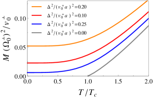
Figure 1: Temperature dependence of the zone center optic phonon frequencies $\Omega_{0}^{\perp}$ for dipole interactions and compositional disorder. The frequencies remain finite down to $T=0$ for finite disorder, thus excluding long-range ferroelectric order.

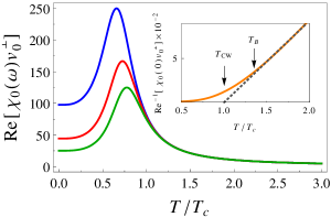
Figure 2: Temperature and frequency dependence of the real part of the dynamic susceptibility $\chi_{0}(\omega)$. Inset: Inverse of the real part of the static susceptibility with compositional disorder ($\Delta^{2}/(v_{0}^{\perp}a)^{2}=0.03$). Deviations from Curie-Weiss law are indicated by the gray dashed line. Blue (top), red (middle), and green (bottom) lines correspond to $\omega\Gamma/v_{0}^{\perp}=2.0\times 10^{-2},~{}3.0\times 10^{-2},~{}4.0\times 10^{-2}$.

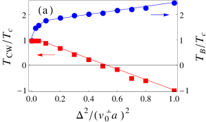
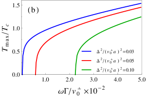
Figure 3: (a) Curie-Weiss ($T_{CW}$) and Burns ($T_{B}$) temperatures dependence on compositional disorder. (b) Frequency and disorder dependence of the temperature $T_{\max}$ at which the dielectric constant is maximum.

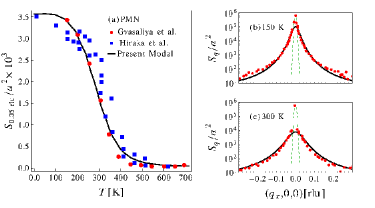
Figure 4: (a) Temperature and (b)-(c) wavevector dependence of the structure factor $S_{\bm{q}}$. Red dots and blue squares correspond to neutron scattering data from Refs. [Gvasaliya2005a, ; Hiraka2004a, ] in the vicinity of the $(110)$ and $(100)$ Bragg peaks in PMN. Black solid line corresponds to the calculated $S_{\bm{q}}$ with $(v_{0}^{\perp}-\kappa)/{v_{0}^{\perp}}=0.85,~{}\gamma a^{2}/v_{0}^{\perp}=0.09,~{}\hbar/(Mv_{0}^{\perp}a^{4})^{1/2}=5.0,~{}\Delta^{2}/(v_{0}^{\perp}a)^{2}=0.03$, and $k_{B}T_{c}/(v_{0}^{\perp}a^{2})=1.0$ with $T_{c}=465\,$K. The green dashed line is a Gaussian Bragg peak of width given by the experimental resolution used in Ref. [Gvasaliya2005a, ] ($\simeq 0.01\,$rlu).

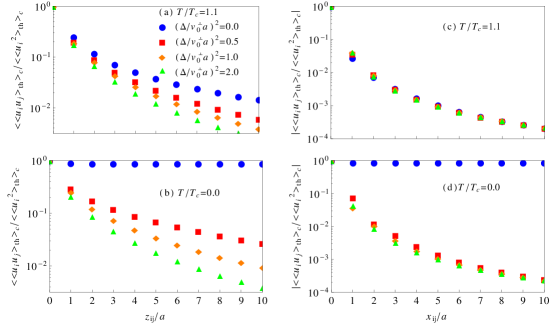
Figure 5: Log-linear plot of near-neighbor correlation functions of polarization for several temperatures and disorder strengths. Here, $(v_{0}^{\perp}-\kappa)/v_{0}^{\perp}=0.40,~{}\gamma a^{2}/v_{0}^{\perp}=0.10$, and $\hbar/(Mv_{0}^{\perp}a^{4})^{1/2}=1.0$.

Associated with the phonon frequency is the dielectric response $\chi_{0}(\omega)$, shown in Fig. 2, where $T_{CW}$ and $T_{B}$ are also identified (see the inset in Fig. 2). Figs. 3 (a)-(b) give the variation of $T_{CW}$, $T_{B}$, and $T_{\max}$ with the parameters of the model. We see that the characteristic temperatures are understood by the ratio of the disorder distribution to the transverse dipole interaction with the damping $\Gamma$ playing a major role for $T_{\max}$. Clearly, our model is too simple to give the dynamics observed in the relaxor susceptibility such as the Vogel-Fulcher behavior. Glazounov1998a Nonetheless, it can capture several of the temperature scales. To get detailed dynamics, one must add the full landscape of potentials and relaxation processes, which have already been considered in the literature. Burton2006a ; Takenaka2013a This is not the aim of the present paper which is concerned with the simpler question of static structure factor. We may add, however, that it is necessary to have the theory of static structure factor well in hand before one can reliably consider the more complicated dynamical problems.

We now compare the static structure factor $S_{\bm{q}}$ with that measured by neutron scattering experiments Gvasaliya2005a ; Hiraka2004a . Without compositional disorder ($\Delta=0$), simple inspection shows that $S_{\bm{q}=0}$ diverges as the mode frequency softens in the vicinity of the critical point $T_{c}$ where long-range ferroelectric order sets in. For finite compositional disorder ($\Delta>0$), $S_{\bm{q}=0}$ remains finite at all temperatures and there is no long-range ferroelectric order. We find this temperature behavior is in agreement with that observed by neutrons in PMN, as shown in Fig. 4 (a). The flat behavior of $S_{\bm{q}}$ at low temperatures ($T\to 0$) is due to zero-point fluctuations: in the classical limit ($\hbar\to 0$), $S_{\bm{q}}$ of Eq. (18) increases with decreasing temperature and is finite at $T=0$.

Figures 4 (b)-(c) compare the calculated wavevector distribution of $S_{\bm{q}}$ with that observed for the relaxor PMN at $T=150\,$K and $T=300\,$K. We use the same value of the model parameters as those of Fig. 4 (a). The observed line shape cannot be described by a simple Lorentzian seen for conventional perovskite ferroelectrics or the “squared Lorentzian” expected for random field models.

We now compute the spatial dependence and anisotropy of the correlation functions of polarization at various characteristic temperatures and various normalized disorder strengths. These spatial correlations have been Fourier transformed to give the static structure factor $S_{\bm{q}}$. One of the purposes of this section is to contrast the correlations of our model to those expected from hypothetical polar nanoregions (PNRs) on which we will comment at the end.

We first consider the correlation functions of polarization at large distances ($|{\bm{R}}_{ij}|\to\infty$). For low temperatures ($T\to 0$) and arbitrarily small but finite disorder ($0<\Delta/(v_{0}^{\perp}a)\ll 1$), the correlations are anisotropic and slowly decaying functions,

$$\overline{\left<u_{i}u_{j}\right>}=\begin{cases}\left(\frac{4\pi}{3}\right)^{2}\frac{\Delta^{2}}{\left(v_{0}^{\perp}\right)^{2}}\times\frac{32\pi^{3}}{v_{BZ}}\frac{(\bar{\chi}_{0}^{\perp})^{3}}{|{\bm{R}}_{ij}|^{3}},&{\bm{R}}_{ij}\parallel\hat{\bm{z}},\\ -\left(\frac{4\pi}{3}\right)^{2}\frac{\Delta^{2}}{\left(v_{0}^{\perp}\right)^{2}}\times\frac{1}{2}\frac{\pi^{3/2}}{v_{BZ}}\frac{(\bar{\chi}_{0}^{\perp})^{3/2}}{|{\bm{R}}_{ij}|^{3}},&{\bm{R}}_{ij}\perp\hat{\bm{z}},\end{cases}$$ (19)

where $\left(\bar{\chi}_{0}^{\perp}\right)^{-1}=(4\pi/3)\left(\chi_{0}^{\perp}\right)^{-1}/v_{0}^{\perp}$ is a small but finite dimensionless inverse susceptibility; and $v_{BZ}$ is the volume of the Brillouin zone. The ratio of the longitudinal to transverse components is proportional (in absolute value) to $\left(\bar{\chi}_{0}^{\perp}\right)^{3/2}$, indicating that the positive longitudinal correlations are stronger than the negative transverse components. This behavior is similar to that of ferroelectrics without random fields. For an uniaxial ferroelectric without compositional disorder and above the critical temperature $T_{c}$, the correlation functions exhibit the same anisotropy, power law decay, and longitudinal to transverse ratio Lines1974a . The correlations of Eq. (19) are, however, in sharp contrast with those of short-range interactions with quenched random fields in three dimensions where the correlation functions decay exponentially. Birgeneau1983a

We now discuss the near-neighbor correlations with compositional disorder. For temperatures slightly above $T_{c}$, the near-neighbor longitudinal correlations with and without disorder show similar decay with an overall strength that decreases with increasing compositional disorder (Fig. 5(a)). This behavior persists down to $T=0$ for finite compositional disorder (Fig. 5(b)). For no disorder, the correlations exhibit the long-range order expected at $T=0$. The correlations in the transverse direction follow similar decay as that of the longitudinal components except that they are negative and significantly weaker (Figs. 5(c)-(d)).

To compare with the idea of PNRs invoked to rationalize the behavior of relaxors, we note that we find that significant correlations develop below the Burns temperature $T_{B}$. However, we do not find a difference in the characteristic behavior at short distances compared to that at long distances, which might have been expected for PNRs. We find that the correlations have a power law behavior which joins smoothly to a short-range part where they must saturate to near the on-site correlations. This is characteristic of the fluctuation regime of any cooperative problem. We have emphasized that relaxors may be looked on as materials in which the fluctuation regime extends from the Burns temperature all the way to $T=0$. We therefore conclude that the diffuse scattering observed by neutrons does not support the qualitative picture of PNRs. Recently, other works have arrived at similar conclusions. Bosak2012a ; Hlinka2012a ; Takenaka2013a We point out, however, that nucleation of local polar domains within the non-polar phase may occur as there are stable ferroelectric states in the free energy. Guzman2013a

V Conclusions

We have used the insight that the frustrating nature of the dipolar interactions (due to their anisotropy) introduced in a perovskite due to a putative displacive transition together with quenched disorder impedes a ferroelectric transition at all temperatures and leads instead to a region of extended ferroelectric fluctuations in PMN. The nature of the dipolar interactions is such that the physics cannot be captured in a mean-field like or two body correlation approximations to the problem. Using a minimal approximation scheme which is able to handle the special nature of the problem, we are able to derive the observed structure factor of the relaxor PMN and relate it to their static and dynamic microscopic properties.

In addition to the difficulties posed to our current theoretical treatment by the complex dynamic processes of relaxors (see Sec. IV), there are several other challenges which should be addressed in future extensions of this work such as the effects of cubic symmetry, of disorder in the bonds (e.g. lattice stiffness and dipole interactions), and of electrostriction. These are all important ingredients of any model that aims to describe of the universality class, Cowley2011a glassiness, Kleemann2014a and ultra-high piezoelectricity piezoelectricity of typical relaxors such as PMN and its solid solutions with conventional ferroelectrics such as PMN-PT.

VI Acknowledgments

This research was partially supported by the University of California Lab Fee Program 09-LR-01-118286-HELF. We thank Peter Littlewood for insightful discussions and other principal investigators with whom this grant was issued: Frances Hellman, Albert Migliori and Alexandra Navrotsky. Work at Argonne National Laboratory is supported by the U.S. Department of Energy, Office of Basic Energy Sciences under contract no. DE-AC02-06CH11357, and work at the University of Costa Rica by Vicerrectoría de Investigación under the project no. 816-B5-220.

References

- (1) R. A. Cowley, S. N. Gvasaliya, S. G. Lushnikov, B. Roessli and G. M. Rotaru, Adv. Phys. 60, 229 (2011).
- (2) A. A. Bokov and Z.-G. Ye, J. Mater. Sci. 41, 31 (2006).
- (3) W. Kleeman, J. Mater. Sci. 41, 129 (2006).
- (4) G. A. Samara, J. Phys.: Condens. Matter 15, R367 (2003).
- (5) L. E. Cross, Ferroelectrics 151, 305 (1994); L. E. Cross, Ferroelectrics 76, 241 (1987).
- (6) G. Burns and B. A. Scott, Solid State Commun. 13, 423 (1973); G. Burns and F. H. Dacol, Solid State Commun. 48, 853 ̵͑(1983͒); G. Burns and F. H. Dacol, Phys. Rev. B 28, 2527 ̵͑(1983͒).
- (7) D. Viehland, S. J. Jang, L. E. Cross and M. Wuttig, Phys. Rev. B 46 8003 (1992).
- (8) G. A. Smolenskii, J. Phys. Soc. Jpn. 28, Suppl. 26 (1970).
- (9) V. Bovtun, S. Kamba, A. Pashkin, M. Savinov, P. Samoukhina, J. Petzelt, I. P. Bykov and M. D. Glinchuk, Ferroelectrics 298, 23 (2004).
- (10) J. Hlinka, J. Petzelt, S. Kamba, D. Noujni and T. Ostapchuk, Phase Transitions 79, 41 (2006).
- (11) A. A. Bokov and Z.-G. Ye J. Adv. Dielec. 2, 1241010 (2012).
- (12) A.E. Glazounov and A.K. Tagantsev, Appl. Phys. Lett. 73, 856 (1998).
- (13) S. N. Gvasaliya, B. Roessli, R. A. Cowley, P. Huber and S. G. Lushnikov, J. Phys.: Condens. Matter 17, 4343 (2005); R. A. Cowley, S. N. Gvasaliya and B. Roessli, Ferroelectrics 378, 53 (2009).
- (14) H. Hiraka, S. -H Lee, P.M. Gehring, Guangyong Xu and G. Shirane, Phys. Rev. B 70, 184105 (2004).
- (15) P. M. Gehring, H. Hiraka, C. Stock, S.-H. Lee, W. Chen, Z.-G. Ye, S. B. Vakhrushev, and Z. Chowdhuri, Phys. Rev. B 79 224109 (2009).
- (16) for reviews, see G. Xu, J. Phys. Conf. Ser. 320, 012081 (2011) and P. M. Gehring, J. Adv. Dielec. 2, 1241005 (2012).
- (17) Y. Imry, S. Ma, Phys. Rev. Lett. 35, 1399 (1975).
- (18) R. Pirc, R. Blinc, Phys. Rev. B 60, 13470 (1999); R. Blinc, J. Dolinsek, A. Gregorovic, B. Zalar, C. Filipic, Z. Kutnjak, A. Levstik, and R. Pirc, Phys. Rev. Lett. 83, 424 (1999).
- (19) V. Westphal, W. Kleemann, M. D. Glinchuk, Phys. Rev. Lett. 68, 847 (1992).
- (20) M. D. Glinchuk, Br. Ceram. Trans. 103, 76 (2004).
- (21) B. P. Burton, E. Cockayne, S. Tinte, and U. V. Waghmare, Phase Transitions 79, 91 (2006).
- (22) S. Tinte, B. P. Burton, E. Cockayne, and U. V. Waghmare Phys. Rev. Lett. 97, 137601 (2006).
- (23) A. R. Akbarzadeh, S. Prosandeev, E. J. Walter, A. Al-Barakaty, and L. Bellaiche, Phys. Rev. Lett. 108, 257601 (2012).
- (24) H. Takenaka, I. Grinberg, and A. M. Rappe, Phys. Rev. Lett. 110, 147602 (2013).
- (25) D. Sherrington, Phys. Rev. B 89, 064105 (2014).
- (26) W. Kleemann, in Mesoscopic Phenomena in Multifunctional Materials, edited by A. Saxena and A. Planes, Springer Series in Materials Science, Vol 198, p. 249 (Springer, Berlin, 2014).
- (27) G. G. Guzmán-Verri, P. B. Littlewood, and C. M. Varma, Phys. Rev. B 88, 134106 (2013).
- (28) L. Onsager, J. Am. Chem. Soc. 58, 1486 (1936).
- (29) W. Cochran, Phys. Rev. Lett. 3, 412 (1959); W. Cochran, Adv. Phys. 9, 387 (1960); P. W. Anderson, Fizika Dielectrikov, ed. G. I. Skanavi (Akad. Nauk SSSR Fizicheskii Inst., im P. N. Levedeva, Moscow, 1960); P. W. Anderson, A Career in Theoretical Physics, (World Scientific Publishing Co., New Jersey, 1994).
- (30) M. E. Lines and A. M. Glass, Principles and Applications of Ferroelectrics and Related Materials (Clarendon Press, Oxford, 1977).
- (31) C. De Dominicis and I. Giardina, Random Fields and Spin Glasses: A Field Theory Approach (Cambridge University Press, Cambridge, 2010).
- (32) A. Aharony and M. E. Fisher, Phys. Rev. B 8, 3323 (1973).
- (33) I. Vilfan and R. A. Cowley, J. Phys. C: Solid State Phys. 18, 5055 (1985).
- (34) J. H. Van Vleck, J. Chem. Phys. 5 320 (1937).
- (35) R. Brout and H. Thomas, Phys. 3, 317 (1967); H. Thomas and R. Brout, J. Appl. Phys. 39, 624 (1968).
- (36) B. I. Halperin and C. M. Varma, Phys. Rev. B 14, 4030 (1976).
- (37) D. P. Belanger and A. P. Young, J. Magn. Magn. Mater. 100, 272 (1992).
- (38) M. Lines, Phys. Rev. B 9, 950 (1974).
- (39) R. J. Birgeneau, H. Yoshizawa, R. A. Cowley, G. Shirane and H. Ikeda, Phys. Rev. B 28, 1438 (1983).
- (40) J. Hlinka, J. Adv. Dielec. 2, 1241006 (2012).
- (41) A. Bosak, D. Chernyshov, S. Vakhrushev, and M. Krischa, Acta Cryst. A68, 117 (2012).
- (42) S.-E. Park and T. R. Shrout, J. Appl. Phys. 82, 1804 (1997).