Efficient method to generate time evolution of the Wigner function for open quantum systems

Abstract

The Wigner function is a useful tool for exploring the transition between quantum and classical dynamics, as well as the behavior of quantum chaotic systems. Evolving the Wigner function for open systems has proved challenging however; a variety of methods have been devised but suffer from being cumbersome and resource intensive. Here we present an efficient fast-Fourier method for evolving the Wigner function, that has a complexity of $O(N\log N)$ where $N$ is the size of the array storing the Wigner function. The efficiency, stability, and simplicity of this method allows us to simulate open system dynamics previously thought to be prohibitively expensive. As a demonstration we simulate the dynamics of both one-particle and two-particle systems under various environmental interactions. For a single particle we also compare the resulting evolution with that of the classical Fokker-Planck and Koopman-von Neumann equations, and show that the environmental interactions induce the quantum-to-classical transition as expected. In the case of two interacting particles we show that an environment interacting with one of the particles leads to the loss of coherence of the other.

I Introduction

The Wigner function is a useful tool in understanding the relationship between quantum systems and their classical counterparts Zachos and Curtright (2005); Curtright et al. (1998, 2001); Bolivar (2004); Polkovnikov (2010), especially for chaotic systems in which visualization in phase-space has been crucial in enabling breakthroughs Heller (1984). The Wigner function is also very useful for studying the quantum-to-classical transition, the process in which classical dynamics emerges as an effective theory from the underlying quantum mechanics Bhattacharya et al. (2000); Habib et al. (2002); Bhattacharya et al. (2003); Zurek (2003); Everitt (2009); Jacobs (2014), and for which open systems play an important role Hillery et al. (1984); Kapral (2006); Petruccione and Breuer (2002); Bolivar (2012); Caldeira (2014).

The equation of motion for the Wigner function is known as Moyal’s equation, and can be written either as an infinite-order partial differential equation or as an integral equation Moyal (1949); Groenewold (1946). Both forms are difficult to solve and, as a result, a plethora of numerical methods for evolving the Wigner function propagation have been developed. These have involved (i) the integral form of Moyal’s equation Barker and Murray (1983); Grønager and Henriksen (1995); Wong (2003); Dittrich et al. (2006, 2010); Sakurai and Tanimura (2014), (ii) reduction of the Moyal equation to a Boltzmann-like equation Brosens and Magnus (2010); Sels et al. (2012), (iii) propagation of Gaussian and coherent states Herman and Kluk (1984); Shimshovitz and Tannor (2012); Dimler et al. (2009); Koch and Frankcombe (2013), (iv) Monte Carlo schemes in which the Wigner function is contracted by averaging over stochastic trajectories of pure-states Shifren and Ferry (2001); Torres et al. (2009); Filinov et al. (1995); Querlioz et al. (2006), and (v) evolving the density matrix in the coordinate representation Gao (1997); Grossmann and Koch (2009).

In this paper we combine a recently developed, elegant formalism for quantum mechanics in phase space Bondar et al. (2012, 2013) with the spectral split operator method Feit et al. (1982). The spectral (fast Fourier transform) method is desirable because it allows one to take advantage of excellent existing libraries, parallelizes well, and is efficient and highly stable. The versatility and effectiveness of the resulting numerical method is illustrated by simulating decoherence and energy dissipation in single- and two-particle systems.

The rest of the paper is organized as follows. The Hilbert phase space formalism that underlies the numerical methods is introduced in Sec. II. In this section we show how master equations for open systems are written in this formalism, as well as the evolution equations that describe classical motion. We also discuss the relationship between the equations describing the quantum and classical evolution. The split-operator technique for evolving the Wigner function is then presented in Sec. III. In Secs. IV and V we illustrate the use of the split operator technique by applying it to a number of examples. Section VI concludes with a brief summary.

II Formalism

II.1 Hilbert phase-space

We first define the following notation. Given continuous variables $a$ and $b$, we write the derivatives with respect to these variables in the following compact form

$$\partial_{a}\equiv\frac{\partial}{\partial a},\;\;\;\partial_{a}^{2}\equiv\frac{\partial^{2}}{\partial a^{2}},\;\;\;\partial_{ab}^{2}\equiv\frac{\partial^{2}}{\partial a\partial b}$$ (1)

We will also use $\bm{a}$ to denote a continuous variable that is distinct from $a$. As is common we use hats to denote quantum operators that correspond to classical observables. Thus, the position operator $\hat{\bm{x}}$ has a continuous spectrum of eigenvalues given by the variable $\bm{x}$, and the corresponding momentum operator is $\hat{\bm{p}}\equiv-i\hbar\bm{\partial}_{\bm{x}}$. We do not use a hat for the density operator, which we denote by $\rho$, and we write the matrix elements of $\rho$ in the compact form $\rho_{\bm{xy}}=\langle\bm{x}|\rho|\bm{y}\rangle$. Finally, for a function $f$ of two variables $x$ and $y$, we use the form $f(x,y)$ as well as the more compact form $f_{xy}$.

With the above notation the unitary evolution for the quantum density operator $\rho$ is given by Gardiner and Zoller (2004)

$$i\hbar\dot{\rho}=[\hat{H}(\hat{\bm{x}},\hat{\bm{p}}),\rho].$$ (2)

where $[\hat{\bm{x}},\hat{\bm{p}}]=i\hbar$ and $\hat{H}$ is the Hamiltonian. In particular, Eq. (2) in the position representation is

$$i\hbar\,\partial_{t}\rho_{\bm{xx^{\prime}}}=\left[H\left(\bm{x},-i\hbar\bm{\partial}_{\bm{x}}\right)-H\left(\bm{x}^{\prime},i\hbar\bm{\partial}_{\bm{x^{\prime}}}\right)\right]\rho_{\bm{xx^{\prime}}}.$$ (3)

The linear change of variables,

$$\bm{x}=x-\mbox{$\frac{\hbar}{2}$}\theta,\qquad\bm{x}^{\prime}=x+\mbox{$\frac{\hbar}{2}$}\theta,$$ (4)

gives the new representation

$$B_{x\theta}=\langle x-\mbox{$\frac{\hbar}{2}$}\theta|\rho|x+\mbox{$\frac{\hbar}{2}$}\theta\rangle,$$ (5)

with the new equation of motion

$$i\hbar\,\partial_{t}B_{x\theta}= \left[H\left(x-\mbox{$\frac{\hbar}{2}$}\theta,i\left[\partial_{\theta}-\mbox{$\frac{\hbar}{2}$}\partial_{x}\right]\right)\right.\left.-H\left(x+\mbox{$\frac{\hbar}{2}$}\theta,i\left[\partial_{\theta}+\mbox{$\frac{\hbar}{2}$}\partial_{x}\right]\right)\right]B_{x\theta}.$$ (6)

Since $\hbar\theta$ has dimensions of length, the function $B_{x\theta}$ was named the “double configuration space representation” by Blokhintsev Blokhintsev (1940); Blokhintsev and Dadyshevsky (1941). Following Blokhintsev it is possible to define the quantity $p$, with dimensions of momentum, as the conjugate variable to $\theta$. In this way we obtain the celebrated Wigner function, $W_{xp}$, related to $B_{x\theta}$ through the Fourier transform:

$$B_{x\theta}= \int W_{xp}\,e^{-ip\theta}dp,\qquad$$ (7)

$$W_{xp}= \frac{1}{2\pi}\int B_{x\theta}\,e^{ip\theta}d\theta.$$ (8)

Note that while $B_{x\theta}$ is in general a complex valued function, $W_{xp}$ is real and can be normalized according to

$$\int W_{xp}\,dx\,dp=1.$$ (9)

Nevertheless, considering that $W_{xp}$ is not necessarily positive, it cannot be interpreted as a true probability distribution (see discussions below).

Using the above definitions we obtain the equation of motion in phase space

$$i\hbar\,\partial_{t}W_{xp}= {[}H\left(x+\mbox{$\frac{i\hbar}{2}$}\partial_{p},p-\mbox{$\frac{i\hbar}{2}$}\partial_{x}\right)-H\left(x-\mbox{$\frac{i\hbar}{2}$}\partial_{p},p+\mbox{$\frac{i\hbar}{2}$}\partial_{x}\right){]}W_{xp}.$$ (10)

The latter can be also expressed in terms of the Moyal star defined as

$$H_{xp}\star W_{xp}\equiv H_{xp}\exp\!\left(\mbox{$\frac{i\hbar}{2}$}\,\overleftarrow{\partial_{x}}\,\overrightarrow{\partial_{p}}-\mbox{$\frac{i\hbar}{2}$}\,\overleftarrow{\partial_{p}}\,\overrightarrow{\partial_{x}}\right)W_{xp},$$ (11)

where the arrows indicate the direction of the derivatives’ action, and we have written $H_{xp}\equiv H(x,p)$. Employing the following identities

$$H_{xp}\star W_{xp} =H\!\left(x+\mbox{$\frac{i\hbar}{2}$}\overrightarrow{\partial_{p}},p-\mbox{$\frac{i\hbar}{2}$}\overrightarrow{\partial_{x}}\right)W_{xp},$$

$$W_{xp}\star H_{xp} =H\!\left(x-\mbox{$\frac{i\hbar}{2}$}\overrightarrow{\partial_{p}},p+\mbox{$\frac{i\hbar}{2}$}\overrightarrow{\partial_{x}}\right)W_{xp},$$ (12)

the equation of motion (10) becomes

$$i\hbar\,\partial_{t}W_{xp}=H_{xp}\star W_{xp}-W_{xp}\star H_{xp},$$ (13)

which is Moyal’s equation Moyal (1949); Zachos and Curtright (2005); Curtright and Zachos (2012).

An abstract formalism that is independent of the particular representation can be introduced by defining an extended four-operator algebra $\hat{x},\hat{p},\hat{\theta},\hat{\lambda}$ satisfying the following commutator relations Bondar et al. (2012, 2013):

$${[}\hat{x},\hat{p}{]}=0,\quad{[}\hat{x},\hat{\lambda}{]}=i,\quad{[}\hat{p},\hat{\theta}{]}=i,\quad{[}\hat{\lambda},\hat{\theta}{]}=0.$$ (14)

We note that the commuting operators $\hat{x}$ and $\hat{p}$, representing position and momentum in the phase space, form a basis for the Koopman-von Neumann representation of classical mechanics Koopman (1931); von Neumann (1932a, b); Mauro (2002). The operators $\hat{\lambda}$ and $\hat{\theta}$ are known as the Bopp operators Boop (1956); Hillery et al. (1984). The four operators (14) can be used to realize the usual canonically-conjugate position and momentum coordinates via

$$\hat{\bm{x}}=\hat{x}-\mbox{$\frac{\hbar}{2}$}\hat{\theta},\qquad\hat{\bm{p}}=\hat{p}+\mbox{$\frac{\hbar}{2}$}\hat{\lambda},$$ (15)

so that $[\hat{\bm{x}},\hat{\bm{p}}]=i\hbar$. Similarly, one can define a mirror quantum algebra as

$$\hat{\bm{x}}^{\prime}=\hat{x}+\mbox{$\frac{\hbar}{2}$}\hat{\theta},\qquad\hat{\bm{p}}^{\prime}=\hat{p}-\mbox{$\frac{\hbar}{2}$}\hat{\lambda},$$ (16)

obeying the commutation relation with the negative sign $[\hat{\bm{x}}^{\prime},\hat{\bm{p}}^{\prime}]=-i\hbar$, while all the other commutators vanish: $[\hat{\bm{x}},\hat{\bm{x}}^{\prime}]=[\hat{\bm{x}},\hat{\bm{p}}^{\prime}]=[\hat{\bm{p}}^{\prime},\hat{\bm{p}}]=[\hat{\bm{p}}^{\prime},\hat{\bm{x}}]=0$.

The four operators $\hat{x}$, $\hat{\theta}$, $\hat{\lambda}$, and $\hat{p}$ can be used to define a Hilbert space that we refer to as the “Hilbert phase space” after Bondar et al. (2013). Specifically, since the self-adjoint operators $\hat{x}$ and $\hat{\theta}$ (respectively $\hat{\lambda}$ and $\hat{p}$) commute, they share a common orthonormal eigenbasis $|x\theta\rangle$ (respectively $|\lambda p\rangle$). These bases are complete so naturally

$$\bm{1}=\int dxd\theta\scalebox{1.3}{$\bm{|}$}x\theta\scalebox{1.4}{$\bm{\rangle}$}\scalebox{1.3}{$\bm{\langle}$}x\theta\scalebox{1.4}{$\bm{|}$}=\int d\lambda dp\scalebox{1.3}{$\bm{|}$}\lambda p\scalebox{1.4}{$\bm{\rangle}$}\scalebox{1.3}{$\bm{\langle}$}\lambda p\scalebox{1.4}{$\bm{|}$},$$ (17)

where $\scalebox{1.3}{$\bm{\langle}$}\lambda p\scalebox{1.3}{$\bm{|}$}x\theta\scalebox{1.3}{$\bm{\rangle}$}=\exp(ip\theta-ix\lambda)/(2\pi)$.

The position and momentum coordinates introduced above, as well as their mirror counterparts allow Eq.(3) to be rewritten in the more abstract form

$$i\hbar\frac{d}{dt}\scalebox{1.3}{$\bm{|}$}\rho\scalebox{1.4}{$\bm{\rangle}$}=\left[H\left(\hat{\bm{x}},\hat{\bm{p}}\right)-H\left(\hat{\bm{x}}^{\prime},\hat{\bm{p}}^{\prime}\right)\right]\scalebox{1.3}{$\bm{|}$}\rho\scalebox{1.3}{$\bm{\rangle}$},$$ (18)

where $\scalebox{1.2}{$\bm{|}$}\rho\scalebox{1.3}{$\bm{\rangle}$}$ is a ket belonging to the Hilbert phase space .

We can realize $\hat{x},\hat{p},\hat{\theta}$, and $\hat{\lambda}$ in terms of differential operators. For example, the phase space representation $x-p$ is accomplished by

$$\hat{x}=x,\quad\hat{p}=p,\quad\hat{\lambda}=-i{\partial_{x}},\quad\hat{\theta}=-i{\partial_{p}},$$ (19)

while, the $x-\theta$ representation requires

$$\hat{x}=x,\quad\hat{p}=i{\partial_{\theta}},\quad\hat{\lambda}=-i{\partial_{x}},\quad\hat{\theta}=\theta.$$ (20)

Other representations can be constructed in a similar fashion.

The Hilbert phase space formalism conveniently unites previously known results regarding phase-space distribution functions. Considering the Hamiltonian form $\hat{H}=\frac{1}{2m}\hat{\bm{p}}^{2}+V(\hat{\bm{x}})$, the abstract equation of motion for the density matrix is

$$i\hbar\frac{d}{dt}\scalebox{1.3}{$\bm{|}$}\rho\scalebox{1.4}{$\bm{\rangle}$}=\left[\frac{\hbar}{m}\hat{p}\hat{\lambda}+V\left(\hat{x}-\mbox{$\frac{\hbar}{2}$}\hat{\theta}\right)-V\left(\hat{x}+\mbox{$\frac{\hbar}{2}$}\hat{\theta}\right)\right]\scalebox{1.3}{$\bm{|}$}\rho\scalebox{1.4}{$\bm{\rangle}$},$$ (21)

for which the $x-\theta$ representation gives a linear partial differential equation

$$i\hbar\,\partial_{t}\scalebox{1.4}{$\bm{|}$}\rho\scalebox{1.4}{$\bm{\rangle}$}_{\!\!x\theta}=\left[\frac{\hbar}{m}\partial^{2}_{x\theta}+V\left(x-\mbox{$\frac{\hbar}{2}$}\theta\right)-V\left(x+\mbox{$\frac{\hbar}{2}$}\theta\right)\right]\scalebox{1.4}{$\bm{|}$}\rho\scalebox{1.4}{$\bm{\rangle}$}_{\!\!x\theta},$$ (22)

where $\scalebox{1.4}{$\bm{|}$}\rho\scalebox{1.4}{$\bm{\rangle}$}_{\!\!x\theta}\equiv\scalebox{1.4}{$\bm{\langle}$}x\theta\scalebox{1.4}{$\bm{|}$}\rho\scalebox{1.4}{$\bm{\rangle}$}$. Since this differential equation is the same as Eq.(6) we have Bondar et al. (2013)

$$B(x,\theta)=\frac{1}{\sqrt{\hbar}}\scalebox{1.4}{$\bm{|}$}\rho\scalebox{1.4}{$\bm{\rangle}$}_{\!\!x\theta}.$$ (23)

Alternatively, the same equation in the usual phase space is

$$i\hbar{\partial_{t}}\scalebox{1.4}{$\bm{|}$}\rho\scalebox{1.4}{$\bm{\rangle}$}_{\!\!xp}=\biggl{[}-i\frac{\hbar}{m}p{\partial_{x}} +V^{+}-V^{-}\biggr{]}\scalebox{1.4}{$\bm{|}$}\rho\scalebox{1.4}{$\bm{\rangle}$}_{\!\!xp},$$ (24)

where $V^{\pm}=V\left(x\pm i\mbox{$\frac{\hbar}{2}$}{\partial_{p}}\right)$ and

$$W(x,p)=\frac{1}{\sqrt{2\pi\hbar}}\scalebox{1.4}{$\bm{|}$}\rho\scalebox{1.4}{$\bm{\rangle}$}_{\!\!xp}.$$ (25)

Equations (22) and (24) illustrate the power of choosing an appropriate representation: The equation of motion in the $x-\theta$ representation is a second-order partial differential equation with the same computational complexity as the two-dimensional Schrödinger equation, while the equation of motion in the $x$-$p$ representation is much more difficult to solve, as either a higher order partial differential equation or an equally challenging integro-differential equation Zachos and Curtright (2005).

In addition to $W(x,p)$ [$x$-$p$ phase space] and $B(x,\theta)$ [$x$-$\theta$ space], the quantum state can be represented by the functions $A(\lambda,\theta)$ and $Z(\lambda,p)$ as

$$A(\lambda,\theta) =\int dx\,e^{-i\lambda x}B(x,\theta),$$ (26)

$$Z(\lambda,p) =\frac{1}{2\pi}\int dxd\theta\,e^{i(p\theta-\lambda x)}B(x,\theta),$$ (27)

where $A(\lambda,\theta)$ is known as the ambiguity function in signal-processing Cohen and Posch (1985), and $Z(\lambda,p)$ can be regarded as the double momentum space representation since $\hbar\lambda$ has the dimensionality of momentum. The connections among all these functions are easily visualized in the following diagram:

(32)

where vertical arrows denote the $\theta\to p$ partial Fourier transforms ( ${\mathcal{F}_{\theta\rightarrow p}}$), while horizontal arrows indicate the $\lambda\to x$ partial Fourier transforms( $\mathcal{F}^{\lambda\rightarrow x}$).

II.2 Open systems

Having reviewed the equations of motion for unitary evolution in the Hilbert phase-space formalism, we now show how to write various standard Markovian master equations in this formalism. If a master equation that describes the interaction with an environment is time-independent then to preserve the positivity of the density matrix it must have the Lindblad form. This means that in addition to the unitary evolution the derivative of $\rho$ contains one or more additional terms of the form Gardiner and Zoller (2004)

$$\mathcal{L}[\rho]=A\rho A^{\dagger}-\mbox{$\frac{1}{2}$}A^{\dagger}A\rho-\mbox{$\frac{1}{2}$}\rho A^{\dagger}A,$$ (33)

where $A$ can be any operator. For a single particle every operator $A$ can be written as a function of the position and momentum operators, so we can write $A(\hat{\bm{x}},\hat{\bm{p}})$. Following the steps leading to Eq.(18), each of the terms in the Lindblad form $\mathcal{L}[\rho]$ can be easily translated to the Hilbert phase-space formalism by using the following rules:

$$A(\hat{\bm{x}},\hat{\bm{p}})\rho\; \Leftrightarrow\;A(\hat{\bm{x}},\hat{\bm{p}})\scalebox{1.3}{$\bm{|}$}\rho\scalebox{1.4}{$\bm{\rangle}$}$$ (34)

$$\rho A(\hat{\bm{x}},\hat{\bm{p}})\; \Leftrightarrow\;A(\hat{\bm{x}}^{\prime},\hat{\bm{p}}^{\prime})\scalebox{1.3}{$\bm{|}$}\rho\scalebox{1.4}{$\bm{\rangle}$},$$ (35)

and the fact that $A(\hat{\bm{x}},\hat{\bm{p}})$ commutes with $B(\hat{\bm{x}}^{\prime},\hat{\bm{p}}^{\prime})$ for every $A$ and $B$. That is, when any operator $A(\hat{\bm{x}},\hat{\bm{p}})$ acts to the right on $\rho$ it acts on $\scalebox{1.3}{$\bm{|}$}\rho\scalebox{1.4}{$\bm{\rangle}$}$ as itself, and when it acts to the left on $\rho$ it acts on $\scalebox{1.3}{$\bm{|}$}\rho\scalebox{1.4}{$\bm{\rangle}$}$ as $A(\hat{\bm{x}}^{\prime},\hat{\bm{p}}^{\prime})$. Note also that in the Hilbert phase-space

$$A(\hat{\bm{x}},\hat{\bm{p}}) =A\left(\hat{x}-\frac{\hbar\hat{\theta}}{2},\hat{p}+\frac{\hbar\hat{\lambda}}{2}\right),$$ (36)

$$A(\hat{\bm{x}}^{\prime},\hat{\bm{p}}^{\prime}) =A\left(\hat{x}+\frac{\hbar\hat{\theta}}{2},\hat{p}-\frac{\hbar\hat{\lambda}}{2}\right).$$ (37)

As an example, the Lindblad operator for the Wigner function is

$$\mathcal{L}[W_{x,p}]= \biggl{[}A\left(x-\mbox{$\frac{\hbar}{2}$}\hat{\theta},p+\mbox{$\frac{\hbar}{2}$}\hat{\lambda}\right)A^{\dagger}\left(x+\mbox{$\frac{\hbar}{2}$}\hat{\theta},p-\mbox{$\frac{\hbar}{2}$}\hat{\lambda}\right)-\mbox{$\frac{1}{2}$}A^{\dagger}\left(x-\mbox{$\frac{\hbar\hat{\theta}}{2}$},p+\mbox{$\frac{\hbar\hat{\lambda}}{2}$}\right)A\left(x-\mbox{$\frac{\hbar\hat{\theta}}{2}$},p+\mbox{$\frac{\hbar\hat{\lambda}}{2}$}\right)\biggr{.}$$

$$-\mbox{$\frac{1}{2}$}A^{\dagger}\left(x+\mbox{$\frac{\hbar\hat{\theta}}{2}$},p-\mbox{$\frac{\hbar\hat{\lambda}}{2}$}\right)A\left(x+\mbox{$\frac{\hbar\hat{\theta}}{2}$},p-\mbox{$\frac{\hbar\hat{\lambda}}{2}$}\right)\biggl{.}\biggr{]}W_{x,p},$$ (38)

where $\hat{\theta}=-i{\partial_{p}}$ and $\hat{\lambda}=-i{\partial_{x}}$.

We now give useful forms for two important master equations. The first is decoherence in the basis of $x$ for which the master equation is Zurek (2003); Habib et al. (2002); Gardiner and Zoller (2004)

$$i\hbar\mathcal{L}[\rho] =-\frac{D}{\hbar^{2}}[\hat{\bm{x}},[\hat{\bm{x}},\rho]]=\frac{2D}{\hbar^{2}}\left(\hat{\bm{x}}\rho\hat{\bm{x}}-\frac{1}{2}\hat{\bm{x}}^{2}\rho-\frac{1}{2}\rho\,\hat{\bm{x}}^{2}\right);$$ (39)

however, it has a particularly simple form in the Hilbert phase space

$$i\hbar\mathcal{L}\left[\scalebox{1.4}{$\bm{|}$}\rho\scalebox{1.4}{$\bm{\rangle}$}\right]= \frac{D}{\hbar^{2}}\left[2(\hat{x}-\hbar\hat{\theta}/2)(\hat{x}+\hbar\hat{\theta}/2)\right.$$

$$\,\,\,\,-(\hat{x}-\hbar\hat{\theta}/2)(\hat{x}-\hbar\hat{\theta}/2)$$

$$\,\,\,\,-\left.(\hat{x}+\hbar\hat{\theta}/2)(\hat{x}+\hbar\hat{\theta}/2)\right]\scalebox{1.4}{$\bm{|}$}\rho\scalebox{1.4}{$\bm{\rangle}$}$$

$$= -D\hat{\theta}^{2}\scalebox{1.4}{$\bm{|}$}\rho\scalebox{1.4}{$\bm{\rangle}$}.$$ (40)

As a result, Blokhintsev’s dynamical equation for a quantum system undergoing decoherence in the position basis reads

$$\partial_{t}B_{x\theta}= \left[\frac{-i}{m}\partial^{2}_{\theta x}+\frac{V^{-}-V^{+}}{i\hbar}-D\theta^{2}\right]B_{x\theta},$$ (41)

with $V^{-}=V(x-\hbar\theta/2)$ and $V^{+}=V(x+\hbar\theta/2)$.

Another widely used master equation is the time-independent approximation to the Caldeira-Legget model Dekker (1977); Caldeira and Leggett (1983); Gardiner and Zoller (2004); Bolivar (2012). This master equation is not strictly correct because it is not in the Lindblad form, but it is good enough for many purposes to describe damping and thermalization of a harmonic oscillator Munro and Gardiner (1996). It is given by

$$i\hbar\hat{\mathcal{D}}[\rho]=-\frac{i\gamma}{\hbar}[\bm{x},[\bm{p},\rho]_{+}]-\frac{2m\gamma kT}{\hbar^{2}}[\bm{x},[\bm{x},\rho]],$$ (42)

Here $[\bm{p},\rho]_{+}$ denotes the anticommutator, $\gamma$ is the damping coefficient and $T$ is the temperature of a bath. The Hilbert phase-space form of this master equation is

$$i\hbar\hat{\mathcal{D}}\scalebox{1.4}{$\bm{|}$}\rho\scalebox{1.4}{$\bm{\rangle}$}=2\gamma(i\hat{\theta}\hat{p}-mkT\hat{\theta}^{2})\scalebox{1.4}{$\bm{|}$}\rho\scalebox{1.4}{$\bm{\rangle}$},$$ (43)

and in the $x$-$\theta$ representation this becomes

$$\partial_{t}B_{x\theta}= \left[\frac{-i}{m}\partial^{2}_{x\theta}+\frac{V^{-}-V^{+}}{i\hbar}-2\gamma\theta\left(\partial_{\theta}+mkT\theta\right)\right]B_{x\theta}.$$ (44)

II.3 Hilbert Phase Space and Classical Dynamics

Classical mechanics can be embedded in the Hilbert phase space. As discussed in Ref. Bondar et al. (2013), when we take the classical limit $\hbar\to 0$ of Eq. (21) we recover the Koopman-von Neumann equation for the classical state $\scalebox{1.4}{$\bm{|}$}\rho\scalebox{1.4}{$\bm{\rangle}$}$ Koopman (1931); von Neumann (1932a, b); Mauro (2002)

$$i\frac{d}{dt}\scalebox{1.3}{$\bm{|}$}\rho\scalebox{1.4}{$\bm{\rangle}$}=\left[\frac{1}{m}\hat{p}\hat{\lambda}-V^{\prime}(\hat{x})\hat{\theta}\right]\scalebox{1.3}{$\bm{|}$}\rho\scalebox{1.4}{$\bm{\rangle}$},$$ (45)

where the position and momentum are given by the commuting operators $\hat{x}$ and $\hat{p}$ [Eq. (14)]. In this limit the $x$-$p$ representation, $\Psi(x,p)=\scalebox{1.4}{$\bm{\langle}$}xp\scalebox{1.4}{$\bm{|}$}\rho\scalebox{1.4}{$\bm{\rangle}$}$, is the classical Koopman-von Neumann “wave-function” which is essentially the square root of the phase-space probability density. It has the differential equation

$$\frac{\partial}{\partial t}\scalebox{1.4}{$\bm{\langle}$}xp\scalebox{1.4}{$\bm{|}$}\rho\scalebox{1.4}{$\bm{\rangle}$}=\left[-\frac{1}{m}p\frac{\partial}{\partial x}+V^{\prime}(x)\frac{\partial}{\partial p}\right]\scalebox{1.4}{$\bm{\langle}$}xp\scalebox{1.4}{$\bm{|}$}\rho\scalebox{1.4}{$\bm{\rangle}$},$$ (46)

Equation (46) can be also obtained by taking the limit $\hbar\to 0$ of the Moyal equation (24) for the Wigner function $W(x,p)$. The corresponding positive phase-space probability density, $\rho(x,p)=|\Psi(x,p)|^{2}$, can be properly normalized

$$\int\rho(x,p)dxdp=1,$$ (47)

and applying the chain rule to the definition of the density $\rho(x,p)$ one obtains the Liouville equation of classical mechanics, which strikingly is identical to that for the classical wave-function $\Psi(x,p)$ Mauro (2002). Since Eq. (46) is the equation obeyed by the classical probability density it is equivalent to an ensemble of Newtonian trajectories, as can be shown via the method of characteristics. The classical evolution leaves the following cumulative function, time invariant

$$C_{\rho}(\gamma,t)=\int_{\rho<\gamma}\rho(x,p,t)\,dxdp.$$ (48)

This statement is proven by slicing the cumulative distribution for an arbitrarily small increment $\delta\gamma$

$$C_{\rho}(\gamma+\delta\gamma,t)-C_{\rho}(\gamma,t)=\int_{\delta R}\!\!\!\!\rho(x,p,t)\,dxdp\approx\gamma\!\int_{\delta R}\!\!\!\!dxdp,$$ (49)

where $\delta R$ is the region $\gamma<\rho<\gamma+\delta\gamma$. The latter integral measures the phase space volume where $\rho(x,p,t)\approx\gamma$, which is preserved according to Liouville’s theorem, implying the time invariance of $C_{\rho}(\gamma,t)$.

The same arguments establish the time independence of the cumulative distribution

$$C_{\Psi}(\gamma,t)=\int_{\Psi<\gamma}\Psi(x,p,t)\,dxdp,$$ (50)

for Koopman-von Neumann dynamics of real valued states $\Psi(x,p,t)$. Note that $\Psi(x,p,t)$ is real for any time time if and only if the initial condition is real. Contrary to classical mechanics, quantum propagation of the Wigner function does not necessarily preserve the cumulative function. For example, a typical effect of quantum decoherence is the eventual elimination of any negativity in the Wigner function,

$$\mathcal{N}_{W}(t)=C_{W}(0,t)=\int_{W<0}W(x,p,t)\,dxdp.$$ (51)

Modern developments and applications of the Koopman-von Neumann classical mechanics can be found in, e.g., Refs. Gozzi (1988); Gozzi et al. (1989); Wilkie and Brumer (1997a, b); Gozzi and Mauro (2002); Mauro (2002); Deotto et al. (2003a, b); Abrikosov et al. (2005); Blasone et al. (2005); Brumer and Gong (2006); Carta et al. (2006); Gozzi and Pagani (2010); Gozzi and Penco (2011); Cattaruzza et al. (2011); Bondar et al. (2012, 2013).

The Fokker-Planck equation of open classical dynamics can also be described in the present formalism

$$i{\partial_{t}}\rho(x,p)=\left[\frac{1}{m}p\hat{\lambda}-V^{\prime}(x)\hat{\theta}-iD\hat{\theta}^{2}\right]\rho(x,p),$$ (52)

where $\hat{\lambda}$ and $\hat{\theta}$ are the differential operators defined in Eq. (19). The classical limit of Eq. (41), governing quantum decoherence, recovers Eq. (52) as further discussed in Sec. IV.

III Spectral Split-Operator Methods

The unitary time-evolution operator, underlying the equation of motion (21), for a time increment $dt$ is

$$U_{dt}=\exp\biggl{(}-idt\left[\frac{\hat{p}\hat{\lambda}}{m}+\frac{V^{-}-V^{+}}{\hbar}\right]\biggr{)}.$$ (53)

This operator can be approximated using the Trotter product Trotter (1959) in the limit of a small time increment either by the first-order scheme

$$U_{dt}=\exp\left(-i\frac{dt}{m}\hat{p}\hat{\lambda}\right)\exp\left(-i\frac{dt}{\hbar}(V^{-}-V^{+})\right)+O(dt^{2}),$$ (54)

or by the second-order scheme Feit et al. (1982)

$$U_{dt}=\exp\left(-i\frac{dt}{2m}\hat{p}\hat{\lambda}\right)\exp\left(-i\frac{dt}{\hbar}(V^{-}-V^{+})\right)\exp\left(-i\frac{dt}{2m}\hat{p}\hat{\lambda}\right)+O(dt^{3}).$$ (55)

Both factorizations are advantageous for numerical evaluations since the time-evolution propagator is expressed as a sequence of Fourier transforms $\mathcal{F}$ [see Eq. (32)] and element-wise multiplications. Thus, the first order scheme propagates the state in the $x$-$p$ representation according to

$$W(t+dt)=\mathcal{F}^{\lambda\to x}\exp\left(-i\frac{dt}{m}p\lambda\right)\mathcal{F}_{\theta\to p}^{x\to\lambda}\exp\left(-i\frac{dt}{\hbar}(V^{-}-V^{+})\right)\mathcal{F}_{p\to\theta}W(t),$$ (56)

where $V^{\pm}=V\left(x\pm\mbox{$\frac{\hbar}{2}$}\theta\right)$ have now become scalar functions, and $\mathcal{F}_{\theta\to p}^{x\to\lambda}=\mathcal{F}_{\theta\to p}\mathcal{F}^{x\to\lambda}=\mathcal{F}^{x\to\lambda}\mathcal{F}_{\theta\to p}$ is a sequence of two Fourier transforms defined in Eq.(32). Numerical propagators for other representations of the Hilbert phase space can be developed in a similar fashion.

If the Wigner function $W(t)$ at a given point in time is stored in an array of length $N=N_{p}\times N_{x}$, then the total complexity of the propagator Eq. (56) is $O(N\log N)$ since it involves a sequence of two Fast Fourier Transforms Frigo and Johnson (2005) of $O(N\log N)$ complexity, and two element-wise multiplications of $O(N)$ complexity. The fast Fourier transform does not exactly coincide with the formal definition of the Fourier transform $\mathcal{F}$ because of the need to have one more element with negative frequency than with positive frequency. For convenience we thus give the propagators explicitly in terms of discrete position and momentum grids. We assume that both grids have an even number of points given respectively by $N_{p}$ and $N_{x}$, and denote the separation of the grid points by $\Delta x$ and $\Delta p$. In particular the grids are given by $x_{n}$ and $p_{n}$ with

$$\Delta x= 2L_{x}/N_{x}\qquad\Delta p=2L_{p}/N_{p}$$ (57)

$$x_{n}= -L_{x}+n\Delta x,\;\;\;n=0,\ldots,N_{x}-1,$$ (58)

$$p_{m}= -L_{p}+m\Delta p,\;\;\;m=0,\ldots,N_{p}-1,$$ (59)

where $L_{x}$ and $L_{p}$ define the window of interest in the phase space. The Wigner function is actually stored with the grid elements in a different order, in that the negative grid points are stored in the second half of the grid. This order is given by $W_{kj}=W(\tilde{x}_{j},\tilde{p}_{k})$ with

$$\tilde{x}_{j} =\left\{\begin{array}[]{ll}x_{j+N_{x}/2}&\mbox{for}\;\;\;j=0,\ldots,\mbox{$\frac{N_{x}}{2}$}-1\\ x_{j-N_{x}/2}&\mbox{for}\;\;\;j=\mbox{$\frac{N_{x}}{2}$},\ldots,N_{x}-1\end{array}\right.$$ (62)

and with the corresponding relationship between $\tilde{p}_{k}$ and $p_{m}$. Note that the Wigner function at the origin of the coordinate system, $W(0,0)$, is now stored at the edge of the grid as $W_{00}$. The reason for this new grid ordering is that it is the natural ordering upon which to apply the fast Fourier transform. It is, of course, not the natural ordering to use in displaying the Wigner function, so we transform from the $j,k$ ordering to the $n,m$ ordering before plotting. This transformation is called an “FFT shift” and is characterized for being a self-inverse function. It is usually provided in libraries that implement the fast Fourier transform. However it should be noted that some implementations of the “FFT shift” store an extra copy of the Wigner function, which can be prohibitively expensive, which is why the user may need to make explicit use of Eq. (62). We provide a Python implementation of the unitary propagation for a single-particle in the Appendix A.

In the case of other representations, e.g., $x-\theta$, the grid discretization step size $\Delta\theta$ is given by

$$\Delta\theta=2\pi/L_{p},\qquad L_{\theta}=\Delta\theta N_{p}/2;$$ (63)

whereas in the $\lambda-p$ representation

$$\Delta\lambda=2\pi/L_{x},\qquad L_{\lambda}=\Delta\lambda N_{x}/2.$$ (64)

If the system’s initial condition is given by a wave function known analytically, then $B(x,\theta)$ can be readily constructed by Eq. (5), whereas the calculation of the corresponding Wigner distribution requires an additional Fourier transform (8).

III.1 Solving master equations

The split-operator method presented above can be extended to handle non-unitary open quantum system dynamics. For example, the first-order split-operator method for evolving the master equation given in Eq. (40) is

$$W(t+dt)=\mathcal{F}^{\lambda\to x}\exp{\left(-\frac{idt}{m}p\lambda\right)}\mathcal{F}^{x\to\lambda}_{\theta\to p}\exp{\left(-\frac{idt}{\hbar}\left[V^{-}-V^{+}\right]-dtD\theta^{2}\right)}\mathcal{F}_{p\to\theta}W(t).$$ (65)

Similar techniques can be used for solving the classical Liouville equation Dattoli et al. (1995, 1996); Gómez et al. (2014), and can be extended to the Koopman-von Neumann equation (46). However, Liouville-like equations can only be solved exactly for a finite time on a fixed grid, due to the development of increasingly fine structure, know as velocity filamentation Kellogg (1965). This issue can be handled by filtering the phase-space distribution so as to remove high-frequency (spatial) structure. In the $x$-$\theta$ representation this results in the following propagation scheme for $\rho(t)$ and $\Psi(t)$ Klimas (1987); Narayan and Klöckner (2009)

$$\left\{\rho(t+dt)\atop\Psi(t+dt)\right\}=\mathcal{F}^{\lambda\to x}\exp{\left(-\frac{idt}{m}p\lambda\right)}\mathcal{F}^{x\to\lambda}_{\theta\to p}\exp{\left(-idtV^{\prime}(x)-\delta D\theta^{2}\right)}\mathcal{F}_{p\to\theta}\left\{\rho(t)\atop\Psi(t)\right\},$$ (66)

valid for both the classical probability density $\rho(x,p)$ and the Koopman-von Neumann wave function $\Psi(x,p)$. This propagator is equivalent to the evolution of the Fokker-Planck equation (52); the diffusion term in the Fokker-Planck equation washes out the fine structure. A similar numerical trick is used to develop efficient numerical methods for the Hamiltonian-Jacobi equation Sethian (1999).

The Caldeira-Legget master equation, Eq. (42), can be implemented by separating the effects of decoherence and dissipation. The second term in Eq. (42), generating decoherence, has already been treated in Eq. (65). The first term in Eq. (42) describes energy exchange with the bath, and could be evaluated by specially designed finite difference schemes Vesely (1994); Collins et al. (2014); Grossmann and Koch (2009), although these require large grid sizes to achieve numerical stability.

To overcome this limitation we now present a stable method enabling, for the first time, higher dimensional simulations (see Sec.V). The time evolution induced by a general dissipator operator $\hat{\mathcal{C}}$ is

$$\scalebox{1.4}{$\bm{|}$}\rho(t+dt)\scalebox{1.4}{$\bm{\rangle}$} =e^{dt\hat{\mathcal{C}}}\scalebox{1.4}{$\bm{|}$}\rho(t)\scalebox{1.4}{$\bm{\rangle}$}$$

$$=\left(1+dt\,\hat{\mathcal{C}}[1+dt\,\hat{\mathcal{C}}/2]\right)\scalebox{1.4}{$\bm{|}$}\rho(t)\scalebox{1.4}{$\bm{\rangle}$}+O(dt^{3}).$$ (67)

For the energy exchange term in the Caldeira-Legget model, Eq. (42), we have $\hat{\mathcal{C}}=2i\gamma\hat{\theta}\hat{p}$. Using Eq. (67) we can propagate the Wigner function in two steps as

$$W(t+dt) =W(t)+2idt\gamma\,\hat{\theta}\hat{p}\,W^{(1)}(t),$$ (68)

$$W^{(1)}(t) =W(t)+idt\gamma\,\hat{\theta}\hat{p}\,W(t)$$ (69)

where a sequence of $\theta\to p$ Fourier transforms is used to calculate the required operator product:

$$\hat{\theta}\hat{p}W(t)=\mathcal{F}_{\theta\to p}\,\theta\,\mathcal{F}_{p\to\theta}\,pW(t).$$ (70)

We note that the second-order scheme (68) is sufficient for the simulations in Sec. IV and V; nevertheless, higher order corrections can be recursively included if needed.

IV Single-particle Systems

In this section, we apply the numerical methods developed in Sec. III to propagate a single-particle under various interactions with the environment. We consider the model for vibrational diatomic molecular dynamics: a particle with mass $m=58752~{}\mbox{a.u.}$ (we use atomic units (a.u.) throughout) moving in a Morse potential given by

$$V(x)=V_{0}[\exp(-2a[x-r_{e}])-2\exp(a[x-r_{e}])],$$ (71)

with $V_{0}=0.6~{}\mbox{eV}=0.0220~{}\mbox{a.u.}$, $a=2.5~{}\mbox{a.u.}$ and $r_{e}=-4.7~{}\mbox{a.u.}$ The Wigner function for the initial state is shown in Fig. 1(a). This initial state corresponds to the first-exited state of the Morse potential displaced by $x_{0}=4.3~{}\mbox{a.u.}$, and is given by

$$\psi_{1}(x)=Nz^{L-n-1/2}e^{-z/2}\left(1-\frac{L\exp(-a[x-x_{0}])}{L-1}\right),$$ (72)

where $L=\sqrt{2mV_{0}}/a$ and $N$ is a normalization constant. This state possesses significant negativity, defined in Eq. (51), and we propagate it according to three different dynamical equations: (i) unitary evolution, Eq. (21), resulting in the final state shown in Fig. 1 (b); (ii) decoherent dynamics given by Eq. (41), resulting in the final state shown in Fig. 1(c); (iii) Evolution under the Caldeira-Legget master equation, Eq. (44), resulting in the final state given in Fig. 1(d).

These simulations provide an opportunity to observe the emergence of the classical world as a result of the interactions with the environment Bhattacharya et al. (2000); Habib et al. (2002); Bhattacharya et al. (2003); Zurek (2003); Everitt (2009); Jacobs (2014). In particular they illustrate how decoherence eliminates the negative regions of the Wigner function. The final state under purely unitary evolution in Fig. 1(b) contains significant negativity (51), while the states in the presence of interactions with the environment evolve to entirely positive states as seen in Figs 1(c) and 1(d).

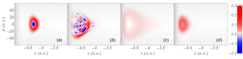
Figure 1: (Color online) Various quantum dynamics in the Morse potential $V(x)$ given in Eq.(71). The contour lines represent level sets of the classical energy $H(x,p)=p^{2}/(2m)+V(x)$. (a) The initial Wigner function (WF) at $t=0~{}\mbox{a.u.}$ (b) The WF at time $t=40,400~{}\mbox{a.u.}$ after unitary evolution employing Eq.(56). (c) The WF at $t=40,400~{}\mbox{a.u.}$ after unitary evolution with additional decoherence in the position basis. The diffusion coefficient is $D=2.70\times 10^{-3}~{}\mbox{a.u.}$ and we use the propagator in Eq.(65). (d) The WF at time $t=40,400~{}\mbox{a.u.}$ after unitary evolution with energy damping given by the Caldeira-Legget model with temperature $T=300K$, diffusion $D=2.70\times 10^{-3}~{}\mbox{a.u.}$ and inverse damping coefficient $\gamma^{-1}=41,341~{}\mbox{a.u.}=1~{}\mbox{ps}$. All these simulations were performed with a grid of $512\times 1024$.

We also propagated the initial state shown in Fig. 1(a) using i) the classical Koopman-von Neumann evolution, Eq. (46), regularized to handle the velocity filamentation (see the discussion in Sec. III ), and ii) the Fokker-Planck evolution (52) with the same diffusion coefficient as used for the open-system evolution shown Fig. 1(c). The result of the Koopman-von Neumann evolution is shown in Fig. 2(a) and that of the Fokker-Planck equation is shown in Fig. 2(b). A comparison of the final states in Fig. 1 and Fig. 2 shows that a quantum state undergoing decoherence converges to the solution of the Fokker-Planck equation, rather than to the corresponding Koopman-von Neumann state. The reason for this is that the decoherence is a measurement process and induces quantum back-action noise that is equivalent to diffusion, and the Fokker-Planck equation correctly includes this diffusion. The classical limit is defined as that in which the action of a system is sufficiently large that the decoherence needed to transform the motion into classical dynamics induces diffusion that is negligible in comparison. In that case the open-system dynamics converges to the Koopman-von Neumann evolution (equivalently the classical Liouville evolution) because the effect off the diffusion is negligible. We note that the color scales in Figs. 1 and 2 differ due to the different normalization conventions for the Wigner function (9) and the Koopman-von Neumann state (47).

While the quantum evolution has a bound on the smallest structure in the phase space Zurek (2001), the Koopman-von Neumann evolution develops an ever finer structure, even for a non-chaotic classical system (see Fig. 2(b)). As a result the Koopman-von Neumann simulations required significantly larger grids than either the quantum or Fokker-Planck simulations.

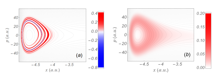
Figure 2: (Color online) (a) Koopman-von Neuman state classically propagated at $t=40400~{}\mbox{a.u.}$, with regularization diffusion coefficient $\delta D=1.5\times 10^{-6}~{}\mbox{a.u.}$ in a grid $768\times 6144$. (b) Corresponding classical state propagated according to the Fokker-Planck equation with decoherence (diffusion) coefficient equal to $D=2.61\times 10^{-3}~{}\mbox{a.u.}$ in a grid $512\times 1024$.

The need to regularize the Koopman-von Neumann propagator, Eq. (66), is illustrated in Fig. 3, where we can see that without regularization the propagator fails to maintain the negativity (Eq. (51)), while the regularized version, in which a small amount of decoherence is added, keeps the negative area approximately constant for long times. In addition, Fig. 3 shows that a larger decoherence rate quickly eliminates all the negativity.

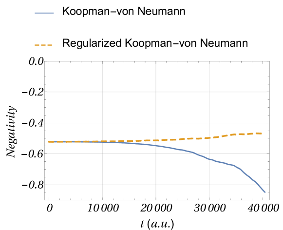
Figure 3: Negativity as a function of time for i) the regularized Koopman-von Neumann propagation with decoherence coefficient $\delta D=1.5\times 10^{-6}~{}\mbox{a.u.}$ (dashed line), ii) Koopman-von Neumann propagation without regularization (solid line), The regularized Koopman-von Neumann propagator maintains an approximately constant negativity, contrary to the monotonic increase given by the un-regularized version.

V Two-particle Systems

A two-particle quantum system in phase space involves four degrees of freedom (i.e., $x$, $p_{x}$, $y$, and $p_{y}$), and has rarely been simulated even for closed system dynamics Filinov et al. (1995); Dittrich et al. (2010). Here we study open system dynamics within the Caldeira-Legget master equation, which has never been attempted, to the best of our knowledge. Even so, we are able to run these simulations on a typical desktop machine. To do this an efficient use of memory becomes critical, and because of this we perform the computations employing single precision arithmetic (32 bit floats). We use a grid which is $128\times 192\times 128\times 192$ and occupies 4.7GB of memory. Two copies of the state are needed according to Eq. (68). The resulting simulation of the Caldeira-Legget evolution remains numerically stable even for the time increment $dt=0.01a.u.$, which is unattainable by alternative methods Vesely (1994); Collins et al. (2014); Grossmann and Koch (2009).

The two particle Wigner function, $W(x,p_{x},y,p_{y})$, expressed through the density matrix

$$W_{2}(x,p_{x},y,p_{y})=\frac{1}{(2\pi)^{2}}\int\langle x-\frac{\hbar}{2}\theta_{x},y-\frac{\hbar}{2}\theta_{y}|\rho|x+\frac{\hbar}{2}\theta_{x},y+\frac{\hbar}{2}\theta_{y}\rangle\,e^{ip_{x}\theta_{x}+ip_{y}\theta_{y}}d\theta_{x}d\theta_{y},$$ (73)

can be reduced to the following single particle Wigner functions,

$$W_{x}(x,p_{x})=\int W_{2}\,dydp_{y},\quad W_{y}(y,p_{y})=\int W_{2}\,dxdp_{x},$$ (74)

which are more easily visualized. Note that even if the two particle state is pure the reduced states may be mixed. The purity of an arbitrary state in the phase space is given by

$$\mathcal{P}=2\pi\int W^{2}(x,p)dxdp,$$ (75)

where the maximum value $\mathcal{P}=1$ is attained for pure states only.

Here we simulate a two particle system evolving in the anharmonic potential

$$V(x,y)=\frac{1}{2}\left(x^{2}+y^{2}\right)+\frac{1}{10}\left(x^{4}+y^{4}+xy\right),$$ (76)

where the first particle interacts with an environment and as result is subject to the Caldeira-Leggett master equation, Eq. (44). The Caldeira-Leggett dynamics is similar to a position measurement because it decoheres the system in the position basis. We chose $D=0.04\,~{}\mbox{a.u.}$ and $\gamma=1./12.5\,~{}\mbox{a.u.}$. The second particle does not interact with the environment, and is only affected by the latter through its interaction with the first particle. Such coupled systems play an important role in describing quantum measurements Wheeler and Zurek (1983); Jacobs and Steck (2006); Jacobs (2014); Clerk et al. (2010); Bose et al. (1999). The initial state is chosen to be an antisymmetric pure entangled state [Figs. 4(a)]

$$\psi_{F}(x,y)= \frac{1}{\sqrt{2}}\left[\psi_{1}(x)\psi_{2}(y)-\psi_{1}(y)\psi_{2}(x)\right],$$ (77)

where $\psi_{1}(x)$ is a Gaussian centered at $x=1$, and $\psi_{2}(x)$ is another Gaussian centered at $y=-1$. Both reduced single particle Wigner functions are identical for this state. However, due to the environment interaction with the first particle, the reduced Wigner functions $W_{x}$ and $W_{y}$ are not equal at later times, and this is shown in Fig. 4(b) and (c). Moreover, $W_{y}$ has a larger negativity than $W_{x}$, indicating that it preserves more of its initial quantum nature. Figure 5 shows how the purity of both reduced states evolves with time.

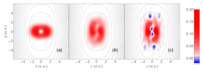
Figure 4: (a) Initial reduced fermionic-like state for both particles ($W_{x}=W_{y}$). (b) Reduced state $W_{x}$ at $t=5.0~{}\mbox{a.u.}$. (c) Reduced state $W_{y}$ at $t=5.0~{}\mbox{a.u.}$.

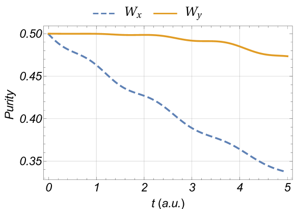
Figure 5: Evolution of the purity for the Fermionic-like reduced states $W_{x}$ (dashed line) and $W_{y}$ (solid line).

VI Conclusion

We have presented a flexible and powerful numerical toolbox for simulating open quantum systems in terms of the Wigner function. These methods significantly reduce the numerical resources required for exact simulation of open systems in phase space, and the method we have presented for solving the Caldeira-Leggett master equation enjoys higher stability than currently available methods. Illustrative examples were provided for single- and two-particle systems that can be evaluated on a typical desktop computer. In these examples we illustrated the emergence of a positive Wigner function as a result of decoherence and compared it with the classical Koopman-von Neumann and Fokker-Planck evolutions. These simulations confirm that quantum evolution with decoherence approaches classical Fokker-Planck dynamics.

Acknowledgments. The authors acknowledge financial support from (HR) NSF CHE 1058644, (RC) DOE DE-FG02-02-ER-15344 and (DB) ARO-MURI W911-NF-11-1-2068.

Appendix A Appendix: Python code for a single particle

⬇

# coding: utf-8

## Wigner Propagator

# In[1]:

import matplotlib.pyplot as plt

from scipy.special import laguerre

import numpy as np

import scipy.fftpack as fftpack

from scipy.special import hyp1f1

# In[2]:

def Fourier_XTheta_to_XP(M):

return fftpack.ifft( M , axis=0 )

# In[3]:

def MorsePsi( n , morse_a, morse_Depth, mass, r0, r):

x = (r-r0)*morse_a

LAMBDA = np.sqrt(2*mass*morse_Depth )/morse_a

z = 2.*LAMBDA*np.exp(-x)

return z**( LAMBDA - n - 0.5 )*np.exp( -0.5*z )*hyp1f1( -n , 2*LAMBDA - 2*n , z )

# In[4]:

def Morse_Wigner(mass, morse_a, morse_Depth, X, Theta):

x_init = -4.3

p_init = 0.

n = 1

psiLeft = MorsePsi(n, morse_a, morse_Depth, mass, x_init, X - 0.5*Theta)

psiRight= MorsePsi(n, morse_a, morse_Depth, mass, x_init, X + 0.5*Theta)

B = psiLeft*psiRight.conj()

W = Fourier_XTheta_to_XP( B )

#norm = np.sum( W )*dX*dP

#W /= norm

return W

# In[5]:

X_gridDIM = 2*512 # Discretization grid size in X

P_gridDIM = 512 # Discretization grid size in P

X_amplitude = 6 # Window range -X_amplitude to X_amplitude

P_amplitude = 80 # Window range -P_amplitude to P_amplitude

dt= 1.01

timeSteps = 1000 # Number of iterations

mass = 32.*1836 # Mass of the particle

# Decoherence parameter

timeDamping = 10.**(-12) * 1./( 2.418884326505*10.**(-17) ) # 1 ps

temperatureT = 300. * 1.3806488*10**(-23) /( 4.35974417*10**(-18) )

gammaDamping = 1./timeDamping

D_Theta = 2*mass*temperatureT*gammaDamping # Decoherence parameter

print ’ gamma = ’, gammaDamping , ’ D_Theta = ’, D_Theta #, ’ D_Lambda = ’, D_Lambda

print ’␣final␣time␣=␣’, timeSteps*dt ,’a.u.␣␣␣=’, timeSteps*dt*2.418884326505*10.**(-17),’␣s’

# Potential parameters

morse_a = 2.5

morse_Depth = 0.6/27.211 # 0.4 eV

morse_x = -4.7

# In[6]:

def truncationFunction(x):

return 1000.*np.arctan( x/1000. )

def Potential(x):

return truncationFunction(

morse_Depth*(np.exp(-2*morse_a*(x-morse_x)) - 2.*np.exp(-morse_a*(x-morse_x ) ) )

)

# In[7]:

# Discretization resolution

dX = 2.*X_amplitude/float(X_gridDIM)

dP = 2.*P_amplitude/float(P_gridDIM)

dTheta = 2.*np.pi/(2.*P_amplitude)

Theta_amplitude = dTheta*P_gridDIM/2.

dLambda = 2.*np.pi/(2.*X_amplitude)

Lambda_amplitude = dLambda*X_gridDIM/2.

# vectors with range of coordinates

X_range = np.linspace(-X_amplitude , X_amplitude -dX , X_gridDIM )

Lambda_range = np.linspace(-Lambda_amplitude , Lambda_amplitude-dLambda , X_gridDIM)

Theta_range = np.linspace(-Theta_amplitude , Theta_amplitude - dTheta , P_gridDIM)

P_range = np.linspace(-P_amplitude , P_amplitude-dP , P_gridDIM)

# matrices of grid of coordinates

X = fftpack.fftshift(X_range)[np.newaxis,:]

Theta = fftpack.fftshift(Theta_range)[:,np.newaxis]

Lambda = fftpack.fftshift(Lambda_range)[np.newaxis,:]

P = fftpack.fftshift(P_range)[:,np.newaxis]

# In[8]:

# Center of the wave packet

x_init = -4.3

p_init = 0.

# Standard deviation in x

mass = 58762

# initialization wigner function

W_init = Morse_Wigner( mass, morse_a, morse_Depth, X, Theta)

norm = np.sum( W_init )*dX*dP

W_init /= norm

# In[9]:

# Ploting potential

fig, ax = plt.subplots(figsize=(10, 5))

ax.plot( X_range, Potential(X_range) )

ax.set_xlim(-5,4)

ax.set_ylim(-0.025,0.001)

ax.set_xlabel(’x’)

ax.set_ylabel(’V’)

ax.grid(’on’)

ax.set_aspect(200.)

# In[10]:

# Matrix grid for the classical Hamiltonian

Hamiltonian_Classical = fftpack.fftshift( P**2/(2*mass) + Potential(X) )

# In[11]:

# Iteration

timeRangeIndex = range(0, timeSteps+1)

print ’␣——————————————————————————-␣’

print ’␣␣␣␣␣Split␣Operator␣Propagator␣␣␣␣␣␣␣␣␣␣␣␣␣␣␣␣␣␣␣␣␣␣␣␣␣␣␣␣␣␣␣␣␣␣␣␣␣␣␣␣␣␣␣␣␣␣␣␣␣␣␣’

print ’␣——————————————————————————-␣’

W = W_init

expPLambda = np.exp(-1j*dt*P*Lambda/mass)

expPotential = np.exp( -dt*1j*(Potential(X-Theta/2.) - Potential(X+Theta/2.)) )

for tIndex in timeRangeIndex:

if tIndex%100==0:

print ’␣␣tIndex␣␣=␣’, tIndex

t = (tIndex)*dt

# p x -> p lambda

W = fftpack.fft( W, axis = 1 )

W *=expPLambda

# p lambda -> p x

W = fftpack.ifft( W, axis = 1 )

# p x -> theta x

W = fftpack.fft( W, axis = 0 )

W *= expPotential

# theta x -> p x

W = fftpack.ifft( W, axis = 0 )

# Normalization

norm = np.sum( W )*dX*dP

W /= norm

W_end = np.real(W)

### Plotting

# In[12]:

def PlotWigner(W):

W = fftpack.fftshift( W )

global_color_max = 0.17 # Maximum value used to select the color range

global_color_min = -0.31 #

print ’min = ’, np.min( W ), ’ max = ’, np.max( W )

print ’normalization␣=␣’, np.sum( W_end )*dX*dP

zero_position = abs( global_color_min) / (abs( global_color_max) + abs(global_color_min))

wigner_cdict = {’red’ : ((0., 0., 0.),

(zero_position, 1., 1.),

(1., 1., 1.)),

’green’ : ((0., 0., 0.),

(zero_position, 1., 1.),

(1., 0., 0.)),

’blue’ : ((0., 1., 1.),

(zero_position, 1., 1.),

(1., 0., 0.)) }

wigner_cmap = plt.cm.colors.LinearSegmentedColormap(’wigner_colormap’, wigner_cdict, 256)

fig, ax = plt.subplots(figsize=(12, 5))

#wigner_cmap = ax.colors.LinearSegmentedColormap(’wigner_colormap’, wigner_cdict, 256)

x_min = -X_amplitude

x_max = X_amplitude - dX

p_min = -P_amplitude

p_max = P_amplitude - dP

cax = ax.imshow( W ,origin=’lower’,interpolation=’none’,

extent=[ x_min , x_max, p_min, p_max],

vmin= global_color_min, vmax=global_color_max, cmap=wigner_cmap)

cbar = fig.colorbar(cax, ticks=[-0.3, -0.2,-0.1, 0, 0.1, 0.2 , 0.3])

ax.set_aspect(1./64.)

ax.set_xlim( -5.3, -3)

ax.contour( Hamiltonian_Classical ,

np.arange(-1, 1, 0.01 ),origin=’lower’,extent=[x_min,x_max,p_min,p_max],

linewidths=0.25,colors=’k’)

return fig

# In[13]:

init_fig = PlotWigner( W_init.real );

init_fig.savefig(”Morse_init.png”);

# In[14]:

end_fig = PlotWigner( W_end.real );

end_fig.savefig(”Morse_end.png”);

# In[14]:

References

- Zachos and Curtright (2005) D. Zachos, C. Fairlie and T. Curtright, Quantum mechanics in phase space: an overview with selected papers, Vol. 34 (World Scientific Publishing Company Incorporated, Singapore, 2005).
- Curtright et al. (1998) T. Curtright, D. Fairlie, and C. Zachos, Phys. Rev. D 58, 025002 (1998).
- Curtright et al. (2001) T. Curtright, T. Uematsu, and C. Zachos, J. Math. Phys. 42, 2396 (2001).
- Bolivar (2004) A. O. Bolivar, Quantum-classical correspondence: dynamical quantization and the classical limit (Springer Verlag, Berlin Heidelberg, 2004).
- Polkovnikov (2010) A. Polkovnikov, Ann. Phys. (NY) 325, 1790 (2010).
- Heller (1984) E. J. Heller, Phys. Rev. Lett. 53, 1515 (1984).
- Bhattacharya et al. (2000) T. Bhattacharya, S. Habib, and K. Jacobs, Phys. Rev. Lett. 85, 4852 (2000).
- Habib et al. (2002) S. Habib, K. Jacobs, H. Mabuchi, R. Ryne, K. Shizume, and B. Sundaram, Phys. Rev. Lett. 88, 040402 (2002).
- Bhattacharya et al. (2003) T. Bhattacharya, S. Habib, and K. Jacobs, Phys. Rev. A 67, 042103 (2003).
- Zurek (2003) W. H. Zurek, Rev. Mod. Phys. 75, 715 (2003).
- Everitt (2009) M. J. Everitt, New J. Phys. 11, 013014 (2009).
- Jacobs (2014) K. Jacobs, Quantum measurement theory and its applications (Cambridge University Press, 2014).
- Hillery et al. (1984) M. Hillery, R. O’Connell, M. Scully, and E. Wigner, Phys. Rep. 106, 121 (1984).
- Kapral (2006) R. Kapral, Ann. Rev. Phys. Chem. 57, 129 (2006).
- Petruccione and Breuer (2002) F. Petruccione and H.-P. Breuer, The theory of open quantum systems (Oxford Univ. Press, 2002).
- Bolivar (2012) A. Bolivar, Ann. Phys. (NY) 327, 705 (2012).
- Caldeira (2014) A. O. Caldeira, An introduction to macroscopic quantum phenomena and quantum dissipation (Cambridge University Press, 2014).
- Moyal (1949) J. Moyal, Math. Proc. Cambridge Philos. Soc. 45, 99 (1949).
- Groenewold (1946) H. Groenewold, Physica 12, 405 (1946).
- Barker and Murray (1983) J. Barker and S. Murray, Phys. Lett. A 93, 271 (1983).
- Grønager and Henriksen (1995) M. Grønager and N. Henriksen, J. Chem. Phys. 102, 5387 (1995).
- Wong (2003) C.-Y. Wong, J. Opt. B: Quantum Semiclassical Opt. 5, S420 (2003).
- Dittrich et al. (2006) T. Dittrich, C. Viviescas, and L. Sandoval, Phys. Rev. Lett. 96, 070403 (2006).
- Dittrich et al. (2010) T. Dittrich, E. Gómez, and L. Pachón, J. Chem. Phys. 132, 214102 (2010).
- Sakurai and Tanimura (2014) A. Sakurai and Y. Tanimura, New J. Phys. 16, 015002 (2014).
- Brosens and Magnus (2010) F. Brosens and W. Magnus, Solid State Commun. 150, 2102 (2010).
- Sels et al. (2012) D. Sels, F. Brosens, and W. Magnus, Phys. A (Amsterdam, Neth.) 391, 78 (2012).
- Herman and Kluk (1984) M. Herman and E. Kluk, Chem. Phys. 91, 27 (1984).
- Shimshovitz and Tannor (2012) A. Shimshovitz and D. J. Tannor, Phys. Rev. Lett. 109, 070402 (2012).
- Dimler et al. (2009) F. Dimler, S. Fechner, A. Rodenberg, T. Brixner, and D. Tannor, New J. Phys. 11, 105052 (2009).
- Koch and Frankcombe (2013) W. Koch and T. J. Frankcombe, Phys. Rev. Lett. 110, 263202 (2013).
- Shifren and Ferry (2001) L. Shifren and D. Ferry, Phys. Lett. A 285, 217 (2001).
- Torres et al. (2009) M. S. Torres, G. Tosi, and J. M. A. Figueiredo, Phys. Rev. E 80, 036701 (2009).
- Filinov et al. (1995) V. Filinov, Y. V. Medvedev, and V. Kamskyi, Mol. Phys. 85, 711 (1995).
- Querlioz et al. (2006) D. Querlioz, J. Saint-Martin, V.-N. Do, A. Bournel, and P. Dollfus, IEEE Trans. Nanotechnol. 5, 737 (2006).
- Gao (1997) S. Gao, Phys. Rev. Lett. 79, 3101 (1997).
- Grossmann and Koch (2009) F. Grossmann and W. Koch, J. Chem. Phys. 130, 034105 (2009).
- Bondar et al. (2012) D. I. Bondar, R. Cabrera, R. R. Lompay, M. Y. Ivanov, and H. A. Rabitz, Phys. Rev. Lett. 109, 190403 (2012).
- Bondar et al. (2013) D. I. Bondar, R. Cabrera, D. V. Zhdanov, and H. A. Rabitz, Phys. Rev. A 88, 052108 (2013).
- Feit et al. (1982) M. Feit, J. Fleck Jr, and A. Steiger, J. Comput. Phys. 47, 412 (1982).
- Gardiner and Zoller (2004) C. Gardiner and P. Zoller, Quantum noise: a handbook of Markovian and non-Markovian quantum stochastic methods with applications to quantum optics, Vol. 56 (Springer, Berlin, Heidelberg, New York, 2004).
- Blokhintsev (1940) D. Blokhintsev, J. Phys. U.S.S.R. 2, 71 (1940).
- Blokhintsev and Dadyshevsky (1941) D. Blokhintsev and Y. B. Dadyshevsky, Zh. Eksp. Teor. Fiz. 11, 222 (1941).
- Curtright and Zachos (2012) T. Curtright and C. Zachos, Asia Pac. Phys. Newsl. 1, 37 (2012).
- Koopman (1931) B. O. Koopman, Proc. Nat. Acad. Sci. U. S. A. 17, 315 (1931).
- von Neumann (1932a) J. von Neumann, Ann. Math. 33, 587 (1932a).
- von Neumann (1932b) J. von Neumann, Ann. Math. 33, 789 (1932b).
- Mauro (2002) D. Mauro, Topics in Koopman-von Neumann Theory, Ph.D. thesis, Università degli Studi di Trieste (2002), arXiv:quant-ph/0301172 .
- Boop (1956) F. Boop, Ann. Inst. H. Poincaré 15 (1956).
- Cohen and Posch (1985) L. Cohen and T. Posch, in Acoustics, Speech, and Signal Processing, IEEE International Conference on ICASSP’85., Vol. 10 (IEEE, 1985) pp. 1033–1036.
- Dekker (1977) H. Dekker, Phys. Rev. A 16, 2126 (1977).
- Caldeira and Leggett (1983) A. Caldeira and A. Leggett, Phys. A (Amsterdam, Neth.) 121, 587 (1983).
- Munro and Gardiner (1996) W. J. Munro and C. W. Gardiner, Phys. Rev. A 53, 2633 (1996).
- Gozzi (1988) E. Gozzi, Phys. Lett. B 201, 525 (1988).
- Gozzi et al. (1989) E. Gozzi, M. Reuter, and W. D. Thacker, Phys. Rev. D 40, 3363 (1989).
- Wilkie and Brumer (1997a) J. Wilkie and P. Brumer, Phys. Rev. A 55, 27 (1997a).
- Wilkie and Brumer (1997b) J. Wilkie and P. Brumer, Phys. Rev. A 55, 43 (1997b).
- Gozzi and Mauro (2002) E. Gozzi and D. Mauro, Ann. Phys. (NY) 296, 152 (2002).
- Deotto et al. (2003a) E. Deotto, E. Gozzi, and D. Mauro, J. Math. Phys. 44, 5902 (2003a).
- Deotto et al. (2003b) E. Deotto, E. Gozzi, and D. Mauro, J. Math. Phys. 44, 5937 (2003b).
- Abrikosov et al. (2005) A. A. Abrikosov, E. Gozzi, and D. Mauro, Ann. Phys. (NY) 317, 24 (2005).
- Blasone et al. (2005) M. Blasone, P. Jizba, and H. Kleinert, Phys. Rev. A 71, 052507 (2005).
- Brumer and Gong (2006) P. Brumer and J. Gong, Phys. Rev. A 73, 052109 (2006).
- Carta et al. (2006) P. Carta, E. Gozzi, and D. Mauro, Ann. Phys. (Berlin, Ger.) 15, 177 (2006).
- Gozzi and Pagani (2010) E. Gozzi and C. Pagani, Phys. Rev. Lett. 105, 150604 (2010).
- Gozzi and Penco (2011) E. Gozzi and R. Penco, Ann. Phys. (NY) 326, 876 (2011).
- Cattaruzza et al. (2011) E. Cattaruzza, E. Gozzi, and A. F. Neto, Ann. Phys. (NY) 326, 2377 (2011).
- Trotter (1959) H. F. Trotter, Proc. Amer. Math. Soc. 10, 545 (1959).
- Frigo and Johnson (2005) M. Frigo and S. G. Johnson, Proc. IEEE 93, 216 (2005).
- Dattoli et al. (1995) G. Dattoli, L. Giannessi, P. L. Ottaviani, and A. Torre, Phys. Rev. E 51, 821 (1995).
- Dattoli et al. (1996) G. Dattoli, P. Ottaviani, A. Segreto, and A. Torre, Nuovo Cimento B 111, 825 (1996).
- Gómez et al. (2014) E. A. Gómez, S. P. Thirumuruganandham, and A. Santana, Comput. Phys. Commun. 185, 136 (2014).
- Kellogg (1965) P. J. Kellogg, Phys. Fluids. 8, 102 (1965).
- Klimas (1987) A. J. Klimas, J. Comp. Phys. 68, 202 (1987).
- Narayan and Klöckner (2009) A. Narayan and A. Klöckner, arXiv preprint arXiv:0911.3589 (2009).
- Sethian (1999) J. A. Sethian, Level SetMethods and Fast Marching Methods (Cambridge University Press, New York, 1999).
- Vesely (1994) F. J. Vesely, Computational Physics: An introduction (Springer, New York, 1994).
- Collins et al. (2014) J. Collins, D. Estep, and S. Tavener, J. Comput. App. Math. 263, 299 (2014).
- Zurek (2001) W. H. Zurek, Nature (London) 412, 712 (2001).
- Wheeler and Zurek (1983) J. A. Wheeler and W. Zurek, Quantum Theory and Measurement (Princeton Series in Physics) (Princeton, NJ: Princeton University Press, 1983).
- Jacobs and Steck (2006) K. Jacobs and D. A. Steck, Contemp. Phys. 47, 279 (2006).
- Clerk et al. (2010) A. Clerk, M. Devoret, S. Girvin, F. Marquardt, and R. Schoelkopf, Rev. Mod. Phys. 82, 1155 (2010).
- Bose et al. (1999) S. Bose, K. Jacobs, and P. L. Knight, Phys. Rev. A 59, 3204 (1999).