Experimental signature of programmable quantum annealing
Abstract
Quantum annealing is a general strategy for solving difficult optimization problems with the aid of quantum adiabatic evolution Finnila et al. (1994); Kadowaki and Nishimori (1998). Both analytical and numerical evidence suggests that under idealized, closed system conditions, quantum annealing can outperform classical thermalization-based algorithms such as simulated annealing Santoro et al. (2002); Morita and Nishimori (2008). Do engineered quantum annealing devices effectively perform classical thermalization when coupled to a decohering thermal environment? To address this we establish, using superconducting flux qubits with programmable spin-spin couplings, an experimental signature which is consistent with quantum annealing, and at the same time inconsistent with classical thermalization, in spite of a decoherence timescale which is orders of magnitude shorter than the adiabatic evolution time. This suggests that programmable quantum devices, scalable with current superconducting technology, implement quantum annealing with a surprising robustness against noise and imperfections.
Many optimization problems can be naturally expressed as the NP-hard problem of finding the ground state, or minimum energy configuration, of an Ising spin glass modelBarahona (1982); Nishimori (2001),
| (1) |
where the parameters and are, respectively, local fields and couplings. The operators are Pauli matrices which assign values to spin values . Two algorithmic approaches designed to address this family of problems are directly inspired by different physical processes: classical simulated annealing (SA), and quantum annealing (QA).
SA Kirkpatrick et al. (1983) probabilistically explores the spin configuration space by taking into account the relative configuration energies and a time-dependent (fictitious) temperature. The initial temperature is high relative to the system energy scale, to induce thermal fluctuations which prevent the system from getting trapped in local minima. As the temperature is lowered, the simulation is driven towards optimal solutions, represented by the global minima of the energy function.
In QA Finnila et al. (1994); Kadowaki and Nishimori (1998) the dynamics are driven by quantum, rather than thermal fluctuations. A system implementing QA Brooke et al. (1999, 2001); Das and Chakrabarti (2008) is described, at the beginning of a computation, by a transverse magnetic field
| (2) |
The system is initialized, at low temperature, in the ground state of , an equal superposition of all computational basis states, the quantum analog of the initial high-temperature classical state. The final Hamiltonian of the computation is the function to be minimized, . During the computation, the Hamiltonian is evolved smoothly from to ,
| (3) |
where the “annealing schedule” satisfies and . If the change is sufficiently slow, the adiabatic theorem of quantum mechanics predicts that the system will remain in its ground state, and an optimal solution is obtained Farhi et al. (2001); Boixo and Somma (2010). Similar transformations with more general Hamiltonians are equivalent in computational power (up to polynomial overhead) to the standard circuit model of quantum computation Aharonov et al. (2007); Mizel et al. (2007), and offer at least a quadratic speed-up over any classical SA algorithm Somma et al. (2008).
Realistically, one should include the effects of coupling to a thermal environment, i.e., consider open system quantum adiabatic evolution Childs et al. (2001); Sarandy and Lidar (2005); Amin et al. (2008); Patanè et al. (2008); de Vega et al. (2010); Albash et al. (2012). An implementation of open system QA has recently been reported in a programmable architecture of superconducting flux qubits Harris et al. (2010); Berkley et al. (2010); Johnson et al. (2010, 2011), and applied to relatively simple protein folding and number theory problems Perdomo-Ortiz et al. (2012); Bian et al. (2012). Although quantum tunneling has already been demonstrated Johnson et al. (2011), the decoherence time in this architecture can be three orders of magnitude faster than the computational timescale, due in part to the constraints imposed by the scalable design. In the circuit model of quantum computation this relatively short decoherence time would imply, without quantum error correction Shor (1995); Chiaverini et al. (2004), that the system dynamics can be described by classical laws Unruh (1995). In the context of open system QA, this might lead one to believe that the experimental results should be explained by classical thermalization, or that in essence QA has effectively degraded into SA.
Here we address precisely this question: are the dynamics in open system QA dominated by classical thermalization with respect to the final Hamiltonian, as in SA, or by the energy spectrum of the time-dependent quantum Hamiltonian? We answer this by studying an eight-qubit Hamiltonian representing a simple optimization problem, and show that classical thermalization and QA make opposite predictions about the final measurement statistics. Our Ising Hamiltonian, depicted in Fig. 1, has a -fold degenerate ground state
| (4a) | ||||
| (4b) | ||||
Sixteen of these states form a cluster of solutions connected by single spin-flips of the ancillae spins [Eq. (4a)], while the seventeenth ground state is isolated from this cluster in the sense that it can be reached only after at least four spin-flips of the core spins [Eq. (4b)]. As we show below, classical thermalization predicts that the isolated solution will be found with higher probability than any of the cluster solutions, i.e., it is enhanced. Furthermore, after an initial transient, faster thermalization corresponds to a higher probability of finding the isolated solution. Open system QA makes the exact opposite prediction: after an initial transient, the isolated solution is suppressed relative to the cluster, and faster quantum dynamics yields higher suppression (lower probability). Our experimental results are consistent with the open system QA prediction of the suppression effect, and inconsistent with classical thermalization. We next discuss these opposite effects, starting from the classical case.
Let denote the probability of state in the cluster (4a), and the probability of the isolated state (4b). The thermalization dynamics are dominated by single spin-flips in our experiment (see Appendix). The probabilities are all close because states in the cluster are connected by single spin flips, so we consider the average cluster probability . Enhancement of the isolated state means that . Our SA numerics show that this is indeed the case for different update rules and cooling schedules, throughout the thermalization evolution (see Appendix). To explain this, note that the general features of a thermalization process are determined by the spectrum of and by the combinatorics of state interconversion. Each of the degenerate ground states can be reached from any other state without ever raising the energy via a sequence of single spin-flips, so that SA never gets trapped in local minima (Appendix).
The SA master equation and the classical thermalization prediction can be derived from first principles from an adiabatic quantum master equation Albash et al. (2012). Let and denote the system and system-bath Hamiltonians. The Lindblad equation is
| (5) | ||||
where , , is the instantaneous eigenbasis of for spin vector , and . We are interested in the thermalization process in which the density operator is diagonal in the computational basis of spin vectors. The system-bath coupling Hamiltonian then has the form , where . We denote by () the spin vector resulting from flipping the th spin up (down). From here we arrive at the classical master equation for the populations :
| (6) |
and the detailed balance condition . Eq. (6) is the master equation that we used in our SA numerics. It can also be used to derive the classical thermalization prediction . To this end, it can be seen directly that the isolated state is connected via single spin-flips to excited states with energy , giving the rate equation . In contrast, all states in the cluster are connected via single spin-flips to at most singly-excited states; the other four spin-flips connect between other states in the cluster and hence conserve the energy. Thus . Comparing, we conclude that population feeds into the isolated state faster than into the cluster and, given that initially , we always observe . Simultaneous double spin-flips do not change this conclusion, and higher order simultaneous spin-flips are physically less likely. A complete derivation is given in the Appendix.
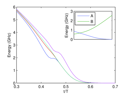
We next analyze the corresponding predictions of QA. A crucial difference with respect to SA is that now the relevant energy spectrum is given by a combination of the final Ising Hamiltonian and the transverse field. Consequently, as shown in Fig. 2, the degeneracy of the ground space is lifted for times . The isolated state has support only on the highest eigenstate plotted during the second half of the evolution. Given that the system starts in the ground state, the isolated state is suppressed by the energy gap, until this gap vanishes at the end of the evolution. The isolated state remains suppressed nonetheless, since transitions to other low energy states require at least four spins-flips. The transverse field term, which drives simultaneous spin-flip transitions, is small at large . If the four spins-flips are not simultaneous, these transitions involve excited states with much higher energy, and are suppressed. This predicted QA suppression of the isolated state is confirmed by our closed and open system quantum dynamical simulations.
Our experiments were performed using the D-Wave One Rainier chip at the USC Information Sciences Institute, comprising unit cells of superconducting flux qubits each, with a total of functional qubits. The couplings are programmable superconducting inductances. The qubits and unit cell, readout, and control have been described in detail elsewhere Harris et al. (2010); Berkley et al. (2010); Johnson et al. (2010, 2011). The initial energy scale for the transverse field is GHz (the function in Fig 2), the final energy scale for the Ising Hamiltonian (the function) is GHz, about fifteen times the experimental temperature of mK GHz. To gather our data, we ran each of the embeddings times, in batches of readouts, resetting all the local fields and couplers after each batch.
A diagram of the experimentally achievable coupling configurations is shown in Fig. 3 (left). The experimental results are shown in Fig. 4. The key finding that is immediately apparent is that the isolated state is robustly suppressed, in agreement with the QA but not the SA prediction.
Is it possible that suppression has an explanation other than QA? The main physical argument along these lines is that a systematic or random bias due to experimental imperfections breaks the -fold ground state degeneracy and energetically disfavors the isolated state, thus lowering if the system thermalizes. We proceed to examine this and the robustness of the suppression effect.
First, note that spin numbers must be assigned to the flux qubits before each experimental run. One of the possible such “embeddings” allowed by the symmetries of the Hamiltonian and the hardware connectivity-graph is shown in Fig. 3 (right).
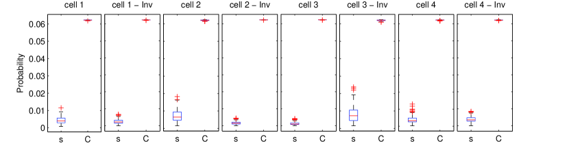
Second, note that spin-inversion transformations commute with , and simply relabel the spectrum of both and : if a certain spin configuration has energy , then the corresponding spin configuration with the th spin flipped has the same energy under . Spin-inversions also commute with the spin-flip operations of classical thermalization. Therefore all of our arguments for the suppression of the isolated state in QA and for its enhancement in classical thermalization are unchanged. Using spin inversions we can check that the suppression effect is not due to a perturbation of the Hamiltonian such as a magnetic field bias. Indeed, by performing a spin-inversion on all spins we obtain a new Ising Hamiltonian where the isolated state is that with all spins-up. If a field bias suppressed the all spins-down state, then it would enhance the all spins-up state. Figure 4 rules this out. We also tested cases with only antiferromagnetic couplings, and with random spin-inversions. The results for one such random inversion example are shown in Fig. 5. In all cases we found agreement with the QA prediction, but not with classical thermalization.
Robust suppression holds even at the level of individual embeddings and spin inversions. We found that %, while % for each of the thousands of such cases we tested (the highest median for the experiment in Fig 4 is 0.004). Thus suppression survives breaking of the ground state degeneracy, which certainly occurs due to the limited precision of % in our control of . The suppression effect is robust because it does not depend on the exact values of these parameters, but on the relatively large Hamming distance between the isolated state and the cluster.
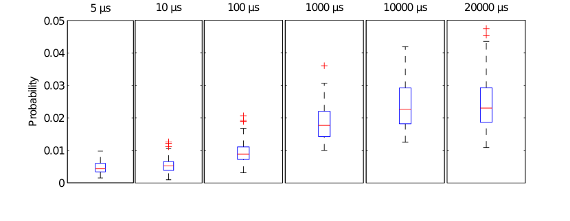
Finally, we consider the effect of increasing the annealing time. Open quantum and classical systems converge towards thermal equilibrium. Therefore if the cause of suppression is the QA spectrum, longer annealing times will result in increasing, approaching its Gibbs distribution value. This would not be the case if were governed by the spectrum of . In Fig. 6 we compare a numerical simulation of open system QA, using an adiabatic Markovian master equation Albash et al. (2012), with classical thermalization. The quantum prediction of increasing is confirmed experimentally, as shown in Fig. 5.

We thus arrive at our main conclusion: signatures of QA, as opposed to classical thermalization, persist for timescales that are much longer than the single-qubit decoherence time (from s to ms vs tens of ns) in programmable devices available with present-day superconducting technology. Our experimental results are also consistent with numerical methods that compute quantum statistics, such as Path Integral Monte Carlo aaaM. Troyer and T. Roennow, private communication.. Our study focuses on demonstrating a non-classical signature in experimental QA. Different methods are required to address the question of experimental computational speedups of open system QA relative to optimal classical algorithms.
Acknowledgements.
We thank M. Amin, T. Landing, T. Murray, J. Preskill, T. Roennow and M. Troyer for useful discussions. We particularly thank M. Amin for discussions that inspired our choice of the Ising Hamiltonian. This research was supported by the Lockheed Martin Corporation. S.B. and D.A.L. acknowledge support under ARO grant number W911NF-12-1-0523. D.A.L. was further supported by the National Science Foundation under grant number CHM-1037992, and ARO MURI grant W911NF-11-1-0268.
Appendix A First-principles derivation of the master equation
Here we derive the master equation used by SA from first principles within the open quantum systems formalism. This motivates classical SA as a model for a system dominated by classical thermalization of the final Ising Hamiltonian.
Let be the time-dependent system Hamiltonian and be the system-bath Hamiltonian. We have previously established that the Lindblad equation within the rotating wave approximation has the form Albash et al. (2012)
| (7) | ||||
where
| (8a) | ||||
| (8b) | ||||
| (8c) | ||||
is the instantaneous eigenbasis of (we have suppressed its explicit time-dependence) for spin vector , where , and
| (9) |
is the Fourier transform of the bath correlation function. The star adornment on the first subscript () is a reminder that the first operator in the bath correlation function is Hermitian-transposed. We have ignored the Lamb shift in Eq. (7) since for a time-dependent Lindblad evolution it amounts to a small perturbation of the system Hamiltonian. We used this form of the master equation for our quantum open system numerical simulations, as detailed elsewhere Albash et al. (2012).
We assume that the system-bath coupling Hamiltonian has the form
| (12) |
where , we identify with and with , and where we neglect higher-order interactions of the form or above. Since is Hermitian we also have , , , , and where the asterisk denotes complex conjugation. In the computational basis of spin vectors , we introduce the notation
| (13) |
which denotes either a flipping of , or if either acts on or acts on . Then
| (14) |
where the function is defined to evaluate to zero also when annihilates . We are interested in classical thermalization, in which the density operator is diagonal in the computational basis , so we set for . Equation (7) then gives . Using indexes and in Eq. (7), where and , and taking the diagonal matrix element, the Lindblad equation becomes
| (15) | ||||
Note that the sum in Eq. (7) involving the resonant contribution vanishes, since the terms and cancel after taking the diagonal matrix element. Moreover, since Eq. (15) involves only off-diagonal terms (), contributions due to all vanish, and using Eq. (14), we are left with
| (16) |
where we denoted , the probability of spin configuration . We can furthermore identify
| (17a) | |||
| (17b) | |||
as the transition probabilities, so that Eq. (16) becomes the rate equation
| (18) |
This can be further simplified using the KMS condition. Indeed, note that, using in Eqs. (9) and (11), we have
| (19) |
Using this along with [Eq. (8c)] and Eq. (10), we have
| (20) |
Therefore Eq. (17) yields
| (21a) | ||||
| (21b) | ||||
This, together with , gives the detailed balance condition for thermalization dynamics
| (22) |
where we introduced transition functions , which we identify with the transition probabilities in Eq. (21).
We can now rewrite Eq. (18) as the classical master equation that we used in our SA numerical simulations
| (23) |
Appendix B Correlation functions and the KMS condition
Here we derive the detailed balance condition Eq. (10) from first principles. Our calculation closely follows Ref. Albash et al., 2012, but differs in that it applies also to non-Hermitian bath operators.
The correlation function of a thermal bath is assumed to satisfy the KMS (Kubo-Martin-Schwinger) condition Breuer and Petruccione (2002)
| (24) |
This expression has the advantage that it also applies to operators which are not trace class. For trace class operators the KMS condition can be derived assuming that the bath is in a thermal state, , where is the bath Hamiltonian. In this case:
| (25) |
where is the bath unitary evolution operator. Note that
| (26) |
If in addition the correlation function is analytic in the strip between and , then it follows that the Fourier transform of the bath correlation function satisfies the detailed balance condition Eq. (10) as we show next.
We compute the Fourier transform:
| (27) |
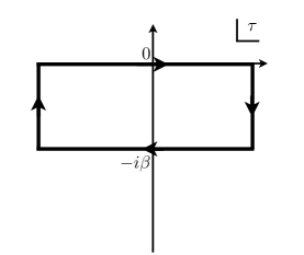
To perform this integral we replace it with a contour integral in the complex plane, , with the contour as shown in Fig. 7. This contour integral vanishes by the Cauchy-Goursat theorem Mathews and Howell (2012) since the closed contour encloses no poles (the correlation function is analytic in the open strip and is continuous at the boundary of the strip Haag et al. (1967)), so that
| (28) | ||||
where is the integrand of Eq. (27), and the integral is the same as in Eq. (27). After making the variable transformation , where is real, we have
| (29) |
Assuming that (i.e., the correlation function vanishes at infinite time), we further have , and hence we find the result:
| (30) | ||||
Appendix C Spectrum and ground states of the Ising Hamiltonian
The spectrum of the -qubit Ising Hamiltonian we consider in the main text,
can be analyzed by first considering the spectrum of the Hamiltonian coupling a single ancilla spin to a core spin, i.e.,
The spectrum, with the core (ancilla) spin written first (second) is
| (35) |
The minimum energy is whether the core spin is up or down. It is important to note that if the core spin is up, the minimum energy is whether the ancilla is up or down; this will give rise to a -fold degeneracy when we account for all spins below.
We analyze the core spins’ energies by first taking into account only their couplings. That is, we analyze the ferromagnetic Hamiltonian
Denoting by the number of satisfied couplings (both spins linked by the coupling have the same sign), the energy is , where . The ground states of this Hamiltonian are the configurations and . Since Eq. (35) shows that the minimum energy of a core-ancilla pair is , when adding the low energy configurations of the couplings to the ancillae the minimum energy is . It also follows from Eq. (35) that the ground state configurations of the full -qubit Hamiltonian are
| (36a) | ||||
| (36b) | ||||
where the first (last) four spins are the core (ancillae) spins, and means that the spin can be either up or down. The all-spins down case (36a) results from the configuration in Eq. (35), while the -fold degenerate case (36b) results from the degeneracy of and.
An important feature of the energy landscape of the -qubit Hamiltonian is that it does not have any local minima. This can be easily proved by showing that a global minimum can always be reached from any state by performing a sequence of single spin flips and never raising the energy. To see this, consider an arbitrary state of the system. We can first flip all the ancillae spins to which, according to Eq. (35), can be done without raising the energy (independently of the state of the corresponding core spin). Then we can flip the core spins in order to satisfy all the couplings between core spins, either making them all or all , whichever requires the fewest spin flips. Again, according to Eq. (35), this operation will not raise the energy of the core-ancilla pair. Hence, the final state is either the isolated ground state , or the state that belongs to the degenerate cluster of ground state configurations.
Appendix D Simulated annealing and classical thermalization
Here we report the results of our numerical simulations of classical thermalization (or SA), using the master equation (23). In the plots below we used the Metropolis update rule for the transition probability . Explicitly, if is the energy difference for the update, the transition probability is
| (37) |
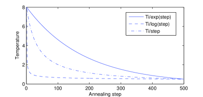
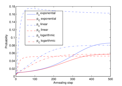
We have also tested other update rules, such as Glauber’s Bertoin et al. (2004), and the results are essentially unchanged. The result are also essentially unchanged when using a transition probability for positive (such as when simulating a continuous time master equation). We do find a dependence on the choice of annealing schedule, i.e., the functional dependence of the temperature on the number of steps. Three different annealing schedules we used are shown in Fig. 8, and the corresponding SA results are shown in Fig. 9. The probability of the isolated state is always above the average probability for a state in the cluster.
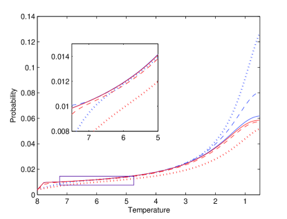
It might be argued that thermalization at constant temperature corresponds most closely to the experimental situation, given that the experimental system remains at an almost constant mK. This is modeled by the exponential annealing schedule, which rapidly converges to a nearly constant temperature, as can be seen in Fig. 8. On the other hand, the energy scale of the Ising model changes during the QA evolution (see the Fig. 2 insert in the main text), and the cooling schedule is determined not by the temperature alone but rather by the ratio between the energy scale and the temperature. We also show and for an exponential schedule with Metropolis updates and different numbers of steps in Fig. 10.
Appendix E Classical master equation explanation for the enhancement of the isolated state
We now explain why, as seen in the numerical simulations shown in Figs. 9 and 10, the probability of the isolated state never exceeds that of the average of the cluster ground states, i.e., why
| (38) |
We are interested in sufficiently slow thermalization processes (relative to spin flip rates), so that states connected by single spin-flips have similar populations. The cluster of degenerate ground states and the isolated ground state are connected via a plateau of excited states with energy .
Let us first derive a rate equation for the isolated state. A single spin-flip of a core spin in the isolated state raises its energy by , since it violates two couplings between the core spins and corresponds to a transition from to (where the second, ancilla, spin is unchanged), which doesn’t change the energy according to Eq. (35). Likewise, a single spin-flip of an ancilla spin in the isolated state violates no couplings and corresponds to a transition from to (with the core spin unchanged), which raises the energy by according to Eq. (35). There are ways this can happen ( core and ancilla spins can be flipped). Since this accounts for all the single spin transitions, Eq. (23) yields the rate equation
| (39) |
where is the population of the excited states with energy . Here we are assuming that the spin flip rate is the same for all sites [corresponding to assuming in Eq. (12)].
We next derive the rate equation for the cluster, once again accounting only for single spin flips. For states in the cluster the core spins are all up, and ancilla-spin flips are energy-preserving transitions between states in the cluster. For core-spin flips we need to analyze two different situations. The first is a configuration in a ground state where the core-ancilla pair starts as and the core spin flips, so the state becomes . This violates two couplings, with energy cost , and according to Eq. (35) the energy difference between these two states is , so the overall result is an excited state with energy . The second is a configuration in a ground state where the core-ancilla pair starts as and again the core spin flips, so the state becomes . This again violates two couplings, with energy cost , but costs no energy according to Eq. (35), so the overall result is an excited state with energy .
Thus, a state with ancillae with spin and ancillae with spin connects (via single spin-flips) to excited states with energy and excited states with energy . To write a rate equation for we shall assume that all excited states with energy () have probability (), and all states in the ground state cluster have equal probability . Summing over the number of ancilla with spin for each cluster state, the rate equation is
| (40a) | ||||
| (40b) | ||||
so that
| (41) |
For most temperatures of interest, relative to the energy scale of the Ising Hamiltonian, the dominant transitions are those between the cluster and states with energy -4. Transitions to energy 0 states are suppressed by the high energy cost, and transitions from energy 0 states to the cluster are suppressed by the low occupancy of the 0 energy states. Then
| (42) |
To show that , assume that this is indeed the case initially. Then, in order for to become larger than , they must first become equal at some inverse annealing temperature : , and it suffices to check that this implies that grows faster than . Subtracting Eq. (42) from Eq. (39) yields
| (43) |
where in the second line we used Eq. (22). Now, because the dynamical SA process we are considering proceeds via cooling, the ratio between the non-equilibrium excited state and the ground state probabilities will not be lower than the corresponding thermal equilibrium transition ratio, i.e., . Therefore, as we set out to show,
| (44) |
implying that at all times .
Appendix F Degenerate perturbation theory explanation for quantum suppression of the isolated state
We can understand the splitting of the degenerate ground subspace of the Ising Hamiltonian by treating the transverse field as a perturbation of the Ising Hamiltonian (thus treating the QA evolution as that of a closed system evolving backward in time). According to standard degenerate perturbation theory, the perturbation of the ground subspace is given by the spectrum of the projection of the perturbation on the ground subspace. Denoting by
| (45) |
the projector on the -dimensional ground subspace, we therefore wish to understand the spectrum of the operator
| (46) |
The isolated state is unconnected via single spin flips to any other state in the ground subspace, so we can write this operator as a direct sum of acting on the isolated state and the projection on the space of the cluster
| (47) |
While acting on any of the four ancillae connects two cluster ground states, acting on any core spin of a cluster state is projected away. Therefore the perturbation is given by the operator
| (48) |
where the sum is over the four ancillae spins.
Denoting the eigenbasis of by , with respective eigenvalues , the transverse field splits the ground space of lowering the energy of , and the four permutations of in the ancillae spins of . None of these states overlaps with the isolated ground state, which is therefore not a ground state of the perturbed Hamiltonian. Furthermore, after the perturbation, only the sixth excited state overlaps with the isolated state. The isolated state becomes a ground state only at the very end of the evolution (with time going forward), when the perturbation has vanished.
Appendix G The quantum Singular Coupling Limit does not agree with the experimental results
Interestingly, an open system QA master equation in the singular coupling limit (SCL) yields results in qualitative agreement with classical thermalization, and opposite to our weak coupling limit (WCL) master equation (7). Here, following Ref. Breuer and Petruccione, 2002, we present a derivation of the SCL master equation.
We consider a Hamiltonian of the form:
| (49) |
where we take the interaction Hamiltonian to have the form , where the system () and bath () operators are both Hermitian. The formal solution in the interaction picture generated by and is given by:
| (50) |
Plugging this solution back into the equation of motion and taking the partial trace over the bath, we obtain:
| (51) |
where we have assumed that . Under the standard Markovian assumption that and under a change of coordinates , we can write:
where and where we have used the homogeneity of the bath correlation function to shift its time-argument. We change coordinates and observe that under this coordinate change is independent of . We assume that this bath correlation function decays in a time that is sufficiently fast, such that . This allows us to approximate the integral by sending the upper limit to infinity. We also assume that , which forces the correlation time of the bath to zero, hence its spectral density to become flat, and hence—using the KMS condition—amounts to taking the infinite temperature limit. Under these assumptions, we can now take the limit, yielding the SCL master equation
| (53) | |||||
where
| (54) | |||||
| (55) |
where is the Lamb shift (renormalization of the system Hamiltonian) and where denotes the Cauchy principal value. Thus, even if is time-dependent, we recover the same form for the SCL master equation as in the time-independent case Breuer and Petruccione (2002). This SCL master equation yields results in qualitative agreement with classical thermalization, and opposite to the WCL presented in Fig. 6 of the main text. Namely, the SCL master equation predicts that the isolated state is enhanced relative to the cluster of states. Since the bath and system-bath coupling dominate the system Hamiltonian in the SCL, it predicts that decoherence takes place not in the instantaneous energy eigenbasis of the system but in the computational basis. Furthermore, the resulting Lamb shift in this limit, diagonal in the computational basis, preferentially lowers the energy of the all-up and all-down states relative to the other computational states. Together, these two effects cause the isolated state to be more populated than the average population of the cluster at the end of the evolution, in contradiction to our experimental findings. The agreement we find between our experimental results and the WCL master equation instead supports the idea that decoherence takes place in the instantaneous energy eigenbasis of the system and/or that the Lamb shift does not dominate the system Hamiltonian.
Appendix H Entanglement
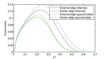
Another interesting question is the possible presence of entanglement during the evolution. Answering this question experimentally requires measurements to be performed during the annealing, a capability that is absent from the device used in our experiments. However, when we compute the concurrence of the states obtained from our master equation (7) during the QA evolution, which is consistent with the statistics of the measured output, we find it to be finite, as seen in Fig. 11. This suggests that entanglement is being generated in our experiments.
References
- Finnila et al. (1994) A. B. Finnila, M. A. Gomez, C. Sebenik, C. Stenson, and J. D. Doll, Chem. Phys. Lett. 219, 343 (1994).
- Kadowaki and Nishimori (1998) T. Kadowaki and H. Nishimori, Phys. Rev. E 58, 5355 (1998).
- Santoro et al. (2002) G. E. Santoro, R. Martonak, E. Tosatti, and R. Car, Science 295, 2427 (2002).
- Morita and Nishimori (2008) S. Morita and H. Nishimori, J. Math. Phys. 49, 125210 (2008).
- Barahona (1982) F. Barahona, J. Phys. A: Math. Gen 15, 3241 (1982).
- Nishimori (2001) H. Nishimori, Statistical Physics of Spin Glasses and Information Processing: An Introduction (Oxford University Press, Oxford, UK, 2001).
- Kirkpatrick et al. (1983) S. Kirkpatrick, C. D. Gelatt, and M. P. Vecchi, Science 220, 671 (1983).
- Brooke et al. (1999) J. Brooke, D. Bitko, T. F. Rosenbaum, and G. Aeppli, Science 284, 779 (1999).
- Brooke et al. (2001) J. Brooke, T. F. Rosenbaum, and G. Aeppli, Nature 413, 610 (2001).
- Das and Chakrabarti (2008) A. Das and B. K. Chakrabarti, Rev. Mod. Phys. 80, 1061 (2008).
- Farhi et al. (2001) E. Farhi, J. Goldstone, S. Gutmann, J. Lapan, A. Lundgren, and D. Preda, Science 292, 472 (2001).
- Boixo and Somma (2010) S. Boixo and R. D. Somma, Phys. Rev. A 81, 032308 (2010), URL http://link.aps.org/doi/10.1103/PhysRevA.81.032308.
- Aharonov et al. (2007) D. Aharonov, W. van Dam, J. Kempe, Z. Landau, S. Lloyd, and O. Regev, SIAM J. Comput. 37, 166 (2007).
- Mizel et al. (2007) A. Mizel, D. A. Lidar, and M. Mitchell, Phys. Rev. Lett. 99, 070502 (2007), URL http://link.aps.org/doi/10.1103/PhysRevLett.99.070502.
- Somma et al. (2008) R. D. Somma, S. Boixo, H. Barnum, and E. Knill, Phys. Rev. Lett. 101, 130504 (2008).
- Childs et al. (2001) A. M. Childs, E. Farhi, and J. Preskill, Phys. Rev. A 65, 012322 (2001).
- Sarandy and Lidar (2005) M. S. Sarandy and D. A. Lidar, Phys. Rev. Lett. 95, 250503 (2005).
- Amin et al. (2008) M. H. S. Amin, P. J. Love, and C. J. S. Truncik, Phys. Rev. Lett. 100, 060503 (2008).
- Patanè et al. (2008) D. Patanè, A. Silva, L. Amico, R. Fazio, and G. E. Santoro, Phys. Rev. Lett. 101, 175701 (2008).
- de Vega et al. (2010) I. de Vega, M. C. Bañuls, and A. Pérez, New J. Phys. 12, 123010 (2010).
- Albash et al. (2012) T. Albash, S. Boixo, D. A. Lidar, and P. Zanardi, arXiv:1206.4197 (2012).
- Harris et al. (2010) R. Harris, M. W. Johnson, T. Lanting, A. J. Berkley, J. Johansson, P. Bunyk, E. Tolkacheva, E. Ladizinsky, N. Ladizinsky, T. Oh, et al., Physical Review B 82, 024511 (2010), URL http://link.aps.org/doi/10.1103/PhysRevB.82.024511.
- Berkley et al. (2010) A. J. Berkley, M. W. Johnson, P. Bunyk, R. Harris, J. Johansson, T. Lanting, E. Ladizinsky, E. Tolkacheva, M. H. S. Amin, and G. Rose, Superconductor Science and Technology 23, 105014 (2010), URL http://stacks.iop.org/0953-2048/23/i=10/a=105014.
- Johnson et al. (2010) M. W. Johnson, P. Bunyk, F. Maibaum, E. Tolkacheva, A. J. Berkley, E. M. Chapple, R. Harris, J. Johansson, T. Lanting, I. Perminov, et al., Superconductor Science and Technology 23, 065004 (2010), URL http://stacks.iop.org/0953-2048/23/i=6/a=065004.
- Johnson et al. (2011) M. W. Johnson, M. H. S. Amin, S. Gildert, T. Lanting, F. Hamze, N. Dickson, R. Harris, A. J. Berkley, J. Johansson, P. Bunyk, et al., Nature 473, 194 (2011).
- Perdomo-Ortiz et al. (2012) A. Perdomo-Ortiz, N. Dickson, M. Drew-Brook, G. Rose, and A. Aspuru-Guzik, Sci. Rep. 2, 571 (2012).
- Bian et al. (2012) Z. Bian, F. Chudak, W. G. Macready, L. Clark, and F. Gaitan (2012), eprint arXiv:1201.1842.
- Shor (1995) P. W. Shor, Phys. Rev. A 52, R2493 (1995).
- Chiaverini et al. (2004) J. Chiaverini, D. Leibfried, T. Schaetz, M. D. Barrett, R. B. Blakestad, J. Britton, W. M. Itano, J. D. Jost, E. Knill, C. Langer, et al., Nature 432, 602 (2004).
- Unruh (1995) W. G. Unruh, Phys. Rev. A 51, 992 (1995), URL http://link.aps.org/doi/10.1103/PhysRevA.51.992.
- Frigge et al. (1989) M. Frigge, D. C. Hoaglin, and B. Iglewicz, The American Statistician 43, 50 (1989), URL http://www.jstor.org/stable/2685173.
- Breuer and Petruccione (2002) H.-P. Breuer and F. Petruccione, The Theory of Open Quantum Systems (Oxford University Press, 2002).
- Mathews and Howell (2012) J. H. Mathews and R. W. Howell, Complex Analysis: for Mathematics and Engineering (Jones and Bartlett Pub. Inc., Sudbury, MA, 2012), sixth ed.
- Haag et al. (1967) R. Haag, N. M. Hugenholtz, and M. Winnink, Comm. Math. Phys. 5, 215 (1967).
- Bertoin et al. (2004) J. Bertoin, F. Martinelli, Y. Peres, and P. Bernard, Lectures on Glauber Dynamics for Discrete Spin Models (Springer Berlin / Heidelberg, 2004), vol. 1717, pp. 93–191.