A Graph Partitioning Approach to Predict Patterns in Lateral Inhibition Systems

Abstract

We analyze pattern formation on a network of cells where each cell inhibits its neighbors through cell-to-cell contact signaling. The network is modeled as an interconnection of identical dynamical subsystems each of which represents the signaling reactions in a cell. We search for steady state patterns by partitioning the graph vertices into disjoint classes, where the cells in the same class have the same final fate. To prove the existence of steady states with this structure, we use results from monotone systems theory. Finally, we analyze the stability of these patterns with a block decomposition based on the graph partition.

I Introduction

Spatial patterning plays a crucial role in multicellular developmental processes [1, 2]. The majority of theoretical results on pattern formation rely on diffusion-driven instabilities, proposed by Turing [3] and further studied by other authors [4, 5, 6]. Although some early events in developmental biology employ diffusible signals, most of the patterning that leads to segmentation and fate-specification relies on contact-mediated signals. Lateral inhibition [7] is a cell-to-cell contact signaling mechanism that leads neighboring cells to compete and diverge to contrasting states of differentiation. An example of lateral inhibition is the Notch pathway, where neighboring cells compete through the interaction between Notch receptors and Delta ligands [8].

Dynamical models for the Notch mechanism have been analyzed in [8] and [9]. However, these either include analytical results for only two cells, or perform numerical simulations for larger networks. A broader dynamical model for lateral inhibition is proposed in [10], and results that are independent of the size of the network are presented. In this reference, the large-scale network is viewed as an interconnection of individual cells, each defined by an input-output model. The contact signaling is represented by an undirected graph, where each vertex is a cell, and a link between two vertices represents the contact between two cells. Results for the instability of the homogeneous steady state and the convergence of two level patterns for bipartite contact graphs are presented in [10].

In this paper, we use the model introduced in [10] and derive results for pattern formation on a general contact graph, recovering the results of [10] for bipartite graphs as a special case. Our main idea is to partition the graph vertices into disjoint classes, where the cells in the same class have the same final fate. We use algebraic properties of the graph and tools from monotone systems theory [11] to prove the existence of steady states that are patterned according to these partitions. Finally, we address the stability of these patterns by decomposing the system into two subsystems. The first describes the dynamics on an invariant subspace defined according to the partition; and the second describes the dynamics transversal to this subspace.

A key property that each partition must satisfy is that the sum of the weights from one vertex in one class to those in another class is independent of the choice of vertex. Partitions with this property are called equitable and allow us to study a reduced model where all vertices in the same class have the same state. As examples of equitable partitions, we study bipartite graphs and graphs with symmetries. For symmetric graphs, we show that subgroups of the automorphism group of a graph can be used to identify equitable partitions.

The idea of grouping the vertices of a network into classes of synchronized states has been explored in [12, 13]; however, no investigation about steady-states and their stability is pursued, and no biological application is addressed. Symmetry properties have been exploited in the dimension reduction and block decomposition of semidefinite program optimization problems, such as fastest mixing Markov chains on the graph [14, 15], and sum-of-squares [16]. Symmetry has also been related to controllability on controlled agreement problems [17].

In Section II, we define the model and introduce necessary graph theoretical concepts. In Section III, we present the main result of the paper, which provides conditions for the existence of steady-state patterns. In Sections IV, we apply the main results to graphs with symmetries, and present examples. Finally, in Section V, we present a decomposition that is helpful for the stability analysis of steady-state patterns, and a small gain stability type criterion.

II Lateral Inhibition Model

We represent the cell network by an undirected and connected graph $\mathcal{G}=\mathcal{G}(V,E)$, where the set of vertices $V$ represents a group of cells, and each edge $e\in E$ represents a contact between two cells. The strength of the contact signal between cells $i$ and $j$ is defined by the nonnegative constant $w_{i,j}$. We let $w_{i,j}=0$ when $i$ and $j$ are not in contact and allow uneven weights to represent distinct contact signal strengths. This contact graph is undirected, i.e., $W=\{w_{ij}\}$ is symmetric.
Let $N$ be the number of cells and define the scaled adjacency matrix $P\in\mathbb{R}^{N\times N}$ of $\mathcal{G}$ as:

$$p_{ij}=d_{i}^{-1}w_{i,j},$$ (1)

where the scaling factor is the node degree $d_{i}=\sum_{j}w_{i,j}$. The definition of $P$ implies that the matrix is nonnegative and row-stochastic, i.e., $P\mathbf{1}_{N}=\mathbf{1}_{N}$, where $\mathbf{1}_{N}\in\mathbb{R}^{N}$ denotes the vector of ones. The structure of $P$ is identical to the transposed probability transition matrix of a reversible Markov Chain. Therefore, $P$ has real valued eigenvalues and eigenvectors.

Consider a network of identical cells $i=1,\ldots,N$ whose dynamical model is given by:

$$\left\{\begin{array}[]{rcl}\dot{x_{i}}&=&f(x_{i},u_{i})\\ y_{i}&=&h(x_{i})\end{array}\right.$$ (2)

where $x_{i}\in\mathcal{X}\subset\mathbb{R}^{n}$ describes the state in cell $i$, $u_{i}\in\mathcal{U}\subset\mathbb{R}$ is an aggregate input from neighboring cells, and $y_{i}\in\mathcal{Y}\subset\mathbb{R}$ represents the output of each cell that contributes to the input to adjacent cells.
We represent the cell-to-cell interaction by

$$u=Py$$ (3)

where $P$ is the scaled adjacency matrix of the contact graph as in (1), $u:=[u_{1}\ldots u_{N}]^{T}$, and $y:=[y_{1}\ldots y_{N}]^{T}$. This means that the input to each cell is a weighted average of the outputs of adjacent cells.

We assume that $f(\cdot,\cdot)$ and $h(\cdot)$ are continuously differentiable, and that for each constant input $u^{*}\in\mathcal{U}$, system (2) has a globally asymptotically stable steady-state

$$x^{*}:=S(u^{*}).$$ (4)

Furthermore, we assume that the map $S:\mathcal{U}\rightarrow\mathcal{X}$ and map $T:\mathcal{U}\rightarrow\mathcal{Y}$, defined as:

$$T(\cdot):=h(S(\cdot)),$$ (5)

are continuously differentiable, and that $T(\cdot)$ is a positive, bounded, and decreasing function. The decreasing property of $T$ is consistent with the lateral inhibition feature, since higher outputs in one cell lead to lower values in adjacent cells.

Note that the steady states of the system (2)-(3) are given by $x_{i}=S(u_{i})$ in which $u_{1},\ldots,u_{N}$ are solutions of the equation:

$$u=P\mathbf{T}_{N}(u),$$ (6)

where

$$\mathbf{T}_{N}(u)=[T(u_{1}),\ldots,T(u_{N})]^{T}.$$ (7)

Since $P$ is row-stochastic, (6) admits the homogeneous solution $u_{i}=u^{*}$ for all $i=1,\ldots,N$, where $u^{*}$ is the unique fixed point of $T(\cdot)$, i.e,

$$T(u^{*})=u^{*}.$$ (8)

III Identifying Steady State Patterns

To identify nonhomogeneous steady states, we introduce the notion of equitable graph partitions. For a weighted and undirected graph $\mathcal{G}(V,E)$ with scaled adjacency matrix $P$, a partition $\pi$ of the vertex set $V$ into classes $O_{1},\ldots,O_{r}$ is said to be equitable if there exist $\overline{p}_{ij}$, $i,j=1,\ldots,r$, such that

$$\sum_{v\in O_{j}}p_{uv}=\overline{p}_{ij}\quad\forall u\in O_{i}.$$ (9)

This definition is a modification of [18, Section 9.3] which considers a partition based on the weights of the graph $w_{ij}$ instead of the scaled weights $p_{ij}$ in (1).

The quotient matrix $\overline{P}\in\mathbb{R}^{r\times r}$ is formed by the entries $\overline{p}_{ij}$. It is also a row-stochastic matrix, and its eigenvalues are a subset of the eigenvalues of $P$, as can be shown with a slight modification of [18, Thm9.3.3]. As we will further discuss, equitable partitions are easy to identify in bipartite graphs, and in graphs with symmetries.

We search for nonhomogeneous solutions to (6) in which the entries corresponding to cells in the same class have the same value. This means that we examine the reduced set of equations

$$z=\overline{P}\mathbf{T}_{r}(z),$$ (10)

where $\overline{P}$ is the quotient matrix of the contact graph $\mathcal{G}$, and $z\in\mathbb{R}^{r}$. The patterns determined from the solutions of (10) are structured in such a way that all cells in the same class have the same fate, i.e,

$$u_{i}=z_{j}\text{ for all }i\in O_{j}.$$ (11)

We now present a procedure to determine if (10) has a nonhomogeneous solution. Define the reduced graph $\mathcal{G}_{\pi}$ to be a simple graph in which the vertex set is $\tilde{V}=\{O_{1},\ldots,O_{r}\}$ and the edge set is

$$\tilde{E}=\{(O_{i},O_{j}):i\neq j,\text{ }\overline{p}_{ij}\neq 0\text{ or }\overline{p}_{ji}\neq 0\}.$$ (12)

Note that we omit self-loops in $\mathcal{G}_{\pi}$ even if $\overline{p}_{ii}\neq 0$.

Assumption III.1

The reduced graph $\mathcal{G}_{\pi}$ is bipartite.

In the following theorem, we determine whether there exists a solution to the reduced set of equations (10) other than the homogeneous solution $z^{*}=u^{*}\mathbf{1}_{r}$.

Theorem III.2

Let $\pi$ be an equitable partition of the vertices of $\mathcal{G}$ such that Assumption III.1 holds. Let $v_{r}$ be the eigenvector of $\overline{P}$ associated with the minimum eigenvalue $\lambda_{r}$. If $T(\cdot)$ is positive, bounded, and decreasing, and if $T^{\prime}(u^{*})$ is such that

$$|T^{\prime}(u^{*})|\lambda_{r}<-1,$$ (13)

then there exists a solution of (10) other than

$$z^{*}=u^{*}\mathbf{1}_{r}.$$ (14)

Proof:

Consider the auxiliary dynamical system:

$$\left[\begin{array}[]{c}\dot{z}_{1}\\ \vdots\\ \dot{z}_{r}\end{array}\right]=-\left[\begin{array}[]{c}z_{1}\\ \vdots\\ z_{r}\end{array}\right]+\overline{P}\left[\begin{array}[]{c}T(z_{1})\\ \vdots\\ T(_{z_{r}})\end{array}\right]:=F(z),\text{ }z\in\mathbb{R}^{r}_{\geq 0}.$$ (15)

Note that around the homogeneous steady state $z^{*}$, the Jacobian matrix

$$DF(z^{*})=-I_{r}+T^{\prime}(u^{*})\overline{P}$$ (16)

is a nonpositive matrix (since $\overline{P}$ is nonnegative, and from (13), $T^{\prime}(u^{*})<0$).
We show that under a coordinate transformation the system is cooperative, see [11, Definition 3.1.3]. Following the bipartite property of $\mathcal{G}_{\pi}$ in Assumption III.1, we define a partition $J\subset\{1,\ldots,r\}$ and $J^{\prime}=\{1,\ldots,r\}\backslash J$ such that no two vertices in the same set are adjacent. Let $\epsilon_{j}=0$ if $j\in J$ and $\epsilon_{j}=1$ if $j\in J^{\prime}$, and choose the transformation $Rz$ to be

$$R=diag\{(-1)^{\epsilon_{1}},\ldots,(-1)^{\epsilon_{j}},\ldots,(-1)^{\epsilon_{r}}\}.$$ (17)

Since the reduced graph is bipartite, $R^{-1}\overline{P}R=R\overline{P}R$ is a matrix similar to $\overline{P}$ and all of its off-diagonal elements are nonpositive. In the new coordinates $Rz$, the Jacobian matrix in (16) becomes $J:=R(DF(z^{*}))R$ and has nonnegative off-diagonal elements. This means that the system is cooperative.
To prove the existence of a solution $\tilde{z}\neq z^{*}$ of (10), we appeal to [11, Theorem 4.3.3] which stipulates that the largest real part of the eigenvalues of $J$ (designated as $s(J)$) to be positive with associated eigenvector $v\gg 0$ (i.e., all elements are positive); and that there exists a bounded forward invariant set.
First, note that $J$ is a quasi-positive and irreducible matrix (this is because the reduced graph is connected, and $T^{\prime}(u^{*})\neq 0$). Then, we know from [11, Corollary 4.3.2] that there exists an eigenvector $v\gg 0$ such that $Jv=s(J)v$. For this case, the eigenvalues of $J$ are all real and given by

$$-1+\lambda_{k}T^{\prime}(u^{*}),\ k=1,\ldots,r,$$ (18)

where $\lambda_{k}$ are the eigenvalues of $\overline{P}$. Therefore, $s(J)=-1+T^{\prime}(u^{*})\lambda_{r}$. From condition (13) we conclude that $s(J)>0$ with positive eigenvector $v$, and that $v_{r}=Rv$ is an eigenvector of $\overline{P}$ associated with $\lambda_{r}$ (i.e., $\overline{P}Rv=\lambda_{r}Rv$).
Second, since the transformed cooperative system is monotone with respect to the standard cone $R^{r}_{\geq 0}$, we conclude that $u^{*}\mathbf{1}_{r}+R^{r}_{\geq 0}$ and $u^{*}\mathbf{1}_{r}-R^{r}_{\geq 0}$ are forward invariant. Furthermore, since $T(\cdot)$ is bounded and decreasing (and $T(u^{*})=u^{*}$), there exists an hypercube $[0,\overline{u}]^{r}$, with $0<u^{*}<\overline{u}$ which is also forward invariant. This can be seen from the fact that at $z=0$, $\dot{z}=\overline{P}T(0)\geq 0$, and at $z=\overline{u}$, $\dot{z}\leq 0$ (since $\overline{u}>T(\overline{u})$). The sets

$$S_{1}=(u^{*}\mathbf{1}+R^{r}_{\geq 0})\cap[0,\overline{u}]^{r}\text{ and }S_{2}=(u^{*}\mathbf{1}-R^{r}_{\geq 0})\cap[0,\overline{u}]^{r},$$ (19)

are forward invariant. Therefore, we conclude from [11, Theorem 4.3.3], there exists an equilibrium point $\tilde{z}\neq z^{*}$, and it satisfies (10). ∎

Example 1: Checkerboard Patterns in Bipartite Graphs
Suppose that the contact graph $\mathcal{G}$ is bipartite, and choose $O_{1}$ and $O_{2}$ to be the partition such that every edge can only connect a vertex in $O_{1}$ to a vertex in $O_{2}$. Then, up to vertex relabeling, the scaled adjacency matrix of $\mathcal{G}$ can be written as

$$P=\left[\begin{array}[]{cc}0&P_{12}\\ P_{21}&0\end{array}\right].$$ (20)

Since the rows of $P_{12}$ (and also rows of $P_{21}$) sum up to $1$, we conclude that $\pi$, consisting of sets $O_{1}$ and $O_{2}$, is an equitable partition. Moreover, the reduced graph $\mathcal{G}_{\pi}$ is itself bipartite (i.e., Assumption III.1 holds), and matrix $\overline{P}$ is given by

$$\overline{P}=\left[\begin{array}[]{cc}0&1\\ 1&0\end{array}\right].$$ (21)

Since the eigenvalues/eigenvectors of $\overline{P}$ are $\lambda_{1}=1$ and $\lambda_{2}=-1$, the next Corollary follows.

Corollary III.3

Let $\mathcal{G}$ be bipartite, and define a partition $O_{1}\subset\{1,\ldots,N\}$ and $O_{2}=\{1,\ldots,N\}\backslash O_{1}$ such that no two vertices in the same set are adjacent. Then, if

$$|T^{\prime}(u^{*})|>1,$$ (22)

there exists a steady state $u=[u_{1}\ldots u_{N}]$ such that $u_{i}=z_{1}$ if $i\in O_{1}$, and $u_{i}=z_{2}$ if $i\in O_{2}$, and $z_{1}\neq z_{2}\neq u^{*}$. $\blacksquare$

The steady state defined by Corollary III.3 results in a “checkerboard” pattern as in Figure 2(A), since it has distinct states for adjacent cells.

IV Graphs with Symmetries

An important class of equitable partitions results from graph symmetries, which are formalized with the notion of graph automorphisms. For a weighted graph $\mathcal{G}(V,E)$, an automorphism is a permutation $g:V\rightarrow V$ such that if $(i,j)\in E$ then also $(gi,gj)\in E$ and $w_{i,j}=w_{gi,gj}$, where $gi$ denotes the image of vertex $i$ under permutation $g$. The set of all automorphisms forms a group designated by automorphism group, $Aut(\mathcal{G})$. A subset $H$ of a full automorphism group $Aut(\mathcal{G})$ is called a subgroup if $H$ is closed under composition and inverse.
Let $H$ be a subgroup of a full automorphism group $Aut(\mathcal{G})$. Then, the action of all permutations $h\in H$ forms a partition of the vertex set into orbits, $O_{i}=\{hi:h\in H\}$, such that $O_{j}=O_{i}$ for all $j\in O_{i}$. Let $r$ be the number of distinct orbits under the subgroup $H$, and relabel them as $\{\overline{O}_{1},\ldots,\overline{O}_{r}\}$. This orbit partition is equitable, because the sum $\sum_{k\in\overline{O}_{j}}p_{i^{*}k}=\overline{p}_{ij}$ is constant independently of the choice of $i^{*}\in\overline{O}_{i}$.
Since any subgroup of the full automorphism group of a graph leads to an equitable partition, we conclude by Theorem III.2 that any orbit partition generated by a subgroup of $Aut(\mathcal{G})$ is a candidate for a pattern structured according to this partition.

Example 2: Two-Dimensional Mesh
Consider a two-dimensional mesh with wraparounds as in Figure 1. Since the graph is bipartite, an equitable partition is given by the two disjoint subsets of vertices $O_{1}=\{1,3,6,8,9,11,14,16\}$, and $O_{2}=\{2,4,5,7,10,12,13,15\}$. From Corollary III.3, we know that a pattern with final value $u_{1}$ for all cells in $O_{1}$, and $u_{2}$ for all cells in $O_{2}$, with $u_{1}\neq u_{2}\neq u^{*}$, is a steady state of the network when $|T^{\prime}(u^{*})|>1$; see Figure 2 (A).

Figure 1: Graph representation for a two-dimensional mesh with wraparounds.

Figure 2: Patterns for the graph in Figure (1).

We next consider the automorphism subgroup that is generated by a combination of two cell rotations in the horizontal direction, one cell rotation in the vertical direction, and one cell rotation in both vertical and horizontal directions. This subgroup leads to the orbits $O_{1}=\{1,3,5,7,10,12,14,16\}$, $O_{2}=\{2,4,6,8,9,11,13,15\}$. The quotient matrix associated with this partition is given by

$$\overline{P}_{B}=\left[\begin{array}[]{cc}\tfrac{1}{4}&\tfrac{3}{4}\\ \tfrac{3}{4}&\tfrac{1}{4}\end{array}\right],$$

and has eigenvalues $-1/2$ and $1$. Therefore, from Theorem III.2, a steady state state given by $z=\overline{P}\mathbf{T}(z)$ exists if $|T^{\prime}(u^{*})|>2$.

In this example, the equitable partition obtained from the bipartite property of the contact graph can also be obtained by a subgroup of the automorphism group of the graph. However, this is in general not true; the four cell path is an example of a graph with a bipartite partition that cannot be defined by an orbit partition.

The computation of automorphism groups, and the identification of the reduced order systems, becomes cumbersome as the size and symmetries of the graphs increase. However, these can be obtained from a computer algebra system with emphasis on computational group theory, such as GAP, [19].

Example 3: Two-dimensional Hexagonal Cyclic Lattice

The number of distinct equitable partitions in a hexagonal lattice of cells is considerably large [20]. We use computational algebra algorithms to find all the possible two-level equitable partitions obtained by automorphisms subgroups in a $6\times 6$ cyclic lattice. Five distinct partitions, each with two classes, are plotted in Figure 3.

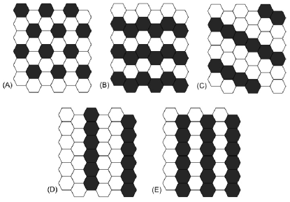
Figure 3: Five distinct partitions, each with two classes, in a $6\times 6$ Two-Dimensional Cyclic Hexagonal Lattice obtained by symmetries on the contact graph.

For these partitions, we have the following scaled adjacency graph of the auxiliary system:

$$\overline{P}_{A}=\left[\begin{array}[]{cc}0&1\\ \tfrac{1}{2}&\tfrac{1}{2}\end{array}\right],\overline{P}_{B}=\left[\begin{array}[]{cc}\tfrac{1}{3}&\tfrac{2}{3}\\ \tfrac{2}{3}&\tfrac{1}{3}\end{array}\right],\overline{P}_{C}=\left[\begin{array}[]{cc}\tfrac{1}{3}&\tfrac{2}{3}\\ \tfrac{1}{3}&\tfrac{2}{3}\end{array}\right],$$

and $\overline{P}_{D}=\overline{P}_{C}$, $\overline{P}_{E}=\overline{P}_{B}$. For each matrix we have the following smallest eigenvalue $\lambda_{A}=-1/2$, $\lambda_{B}=\lambda_{E}=-1/3$, and $\lambda_{C}=\lambda_{D}=0$. We thus conclude from Theorem III.2 that the steady-state represented by pattern $A$ in Figure 3 exists when $|T^{\prime}(u^{*})|>2$, and patterns $B,E$ are steady-states when $|T^{\prime}(u^{*})|>3$. Theorem III.2 is inconclusive for patterns $C,D$.

Example 4: Soccerball Pattern on a Buckminsterfullerene Graph

The next example addresses a larger graph, with 32 cells. It is motivated by the truncated icosahedron solid, also known as the Buckminsterfullerene [18], formed by 12 regular pentagonal faces, and 20 regular hexagonal faces, see Figure 4. In this case, we assume that each face is a vertex and that two vertices are connected if the corresponding faces have a common edge.

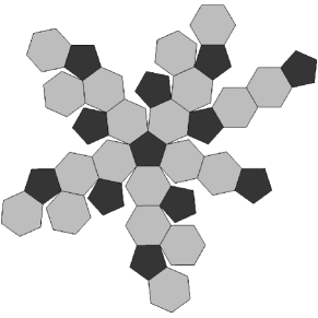
Figure 4: Cell network and soccer ball pattern for the Buckminsterfullerene graph.

The full automorphism group leads to two orbits, one that consists of all the regular pentagon cells ($O_{P}$), and the second orbit encloses all the regular hexagon cells ($O_{H}$). The quotient matrix associated with the orbit partition is then

$$\overline{P}=\left[\begin{array}[]{cc}0&1\\ 1/2&1/2\end{array}\right].$$ (23)

This matrix has eigenvalues $1$ and $-1/2$. Therefore, we conclude from Theorem III.2, that a steady state as in Figure 4 exists when $|T^{\prime}(u^{*})|>2$.

Example 5: Nonbipartite nor Symmetric Equitable Partition
As discussed above, both bipartitions and automorphism subgroups (symmetries) lead to equitable partitions. However, these are not the only cases that lead to equitable partitions. Consider the graph in Figure 5 with partition $C_{1}=\{3,6\}$, and $C_{2}=\{1,2,4,5,7,8\}$. This partition is equitable, but it does not result from an automorphism subgroup (for instance, there is no automorphism exchanging vertices $1$ and $4$), and the graph is also not bipartite (due to the odd length cycles).

$$\overline{P}=\left[\begin{array}[]{cc}0&1\\ 1/2&1/2\end{array}\right]$$

Figure 5: Example of an equitable partition that is neither bipartite nor a symmetry ($C_{1}=\{3,6\}$, $C_{2}=\{1,2,4,5,7,8\}$).

The quotient matrix is the same as in Example 4, we conclude that a two level steady state pattern formed by cells $C_{1}$ and $C_{2}$ exists when $|T^{\prime}(u^{*})|>2$.

V Stability Analysis of Patterns

In the previous sections we discussed the existence of nonhomogeneous steady states for the cell network (2)-(3). Determining stability for these steady states may become cumbersome for a large network of cells. To simplify this task, we decompose the system into an appropriate interconnection of lower order subsystems, and make the interconnection structure explicit.

V-A Network Decomposition

Note that an equitable partition defines the subspace $x_{i}=x_{j}$ for vertices $i$ and $j$ in the same class. This subspace is invariant for the full system (2)-(3). Therefore, the steady states identified using an equitable partition of the contact graph lie on the corresponding invariant subspace. For a partition of dimension $r$, ($O_{1},\ldots,O_{r}$), the reduced order dynamics on this subspace consists of $r$ subsystems as defined in (2), coupled by $u=\overline{P}y$.
Let the steady state be defined by $x_{i}=S(u_{i})$, $i=1,\ldots,N$, where $u_{i}=z_{j}$ if $i\in O_{j}$ and $[z_{1},\ldots,z_{r}]$ is a solution of (10). The linearization at this steady state has the form

$$\dot{x}=(A+BPC)x,$$ (24)

where $A\in\mathbb{R}^{Nn\times Nn}$ is a block diagonal matrix where the $i$-th block is equal to $A_{j}$ if $i$ is in orbit $O_{j}$, and $A_{j}\in\mathbb{R}^{n\times n}$, is given by:

$$A_{j}=\frac{\partial f(x,u)}{\partial x}|_{(x_{j},u_{j})}.$$ (25)

Similarly, $B\in\mathbb{R}^{Nn\times N}$ and $C\in\mathbb{R}^{N\times Nn}$ are block diagonal matrices as in $A$, with $B_{j}=\frac{\partial f(x,u)}{\partial u}|_{(x_{j},u_{j})}$, and $C_{j}=\frac{\partial h(x)}{\partial x}|_{x_{j}}$.
To decompose (24) into two subsystems, we select a representative vertex $V_{i}$ for each class $O_{i}$. The set of $r$ representatives of each class defines the state of the subsystem on the invariant subspace. To see this, let $Q$ be a matrix in $\mathbb{R}^{N\times r}$, where $q_{ij}=1$ if cell $i$ is in class $j$, and $q_{ij}=0$ otherwise. Since the partition is equitable, we conclude that

$$PQ=Q\overline{P}.$$ (26)

Letting $T:=[Q\ R]$ and choosing $R$ to be a matrix in $\mathbb{R}^{N\times(N-r)}$ with columns that, together with those of $Q$, form a basis for $\mathbb{R}^{N}$, we conclude that there exist matrices $C$ and $M$ such that

$$P[\begin{array}[]{cc}Q&R\end{array}]=[\begin{array}[]{cc}Q&R\end{array}]\left[\begin{array}[]{cc}\overline{P}&C\\ 0&M\end{array}\right]:=T\tilde{P}.$$ (27)

The matrix $T$ is invertible and, thus, defines a similarity transformation from matrix $P$ to $\tilde{P}$. Note that the upper left diagonal block of $\tilde{P}$ is the matrix $\overline{P}$, which describes the reduced order subsystem defined by the representative vertices.

Next, we study a particular choice of the matrix $R$ that gives a meaningful variable representation to the transverse subspace dynamics. Let the columns of $R$ be given by standard vectors $e_{i}$, defined as $e_{ij}=\delta_{ij}$, $j=1,\ldots,N$; and further select the columns of $R$ to be $e_{i}$, $i\in\{O_{1}\backslash V_{1},\ldots,O_{r}\backslash V_{r}\}$, in such a way that if $i\in O_{p}\backslash V_{p}$, $j\in O_{q}\backslash V_{q}$, and $p<q$, then $e_{i}$ is in a column before $e_{j}$, i.e., the column with non-zero entry $i$ is placed before the column with entry $j$ if vertex $i$ is in a class with smaller index than the class of vertex $j$.
For this choice of $R$ we conclude from [21, Section 5.3] that the change of variables $T\otimes I_{n}$, i.e., $\tilde{x}=(T^{-1}\otimes I_{n})x$, leads to the decomposition of the linearized dynamics into the subsystem of the $r$ representative cells $V_{i}$ defining the invariant subspace, and the transverse subspace that is defined by the state difference between all the other cells in a class and their corresponding class representative:

$$\tilde{x}_{i}=\left\{\begin{array}[]{rl}x_{V_{i}},&i=1,\ldots,r\\ x_{k}-x_{V_{j}},&i=r+1,\ldots,N\end{array}\right.,\text{ where }k\in O_{j}\backslash V_{j}.$$ (28)

Therefore, the linearized system is decomposed into the representative subsystem $S_{R}$ and the transverse subsystem $S_{D}$,

$$S_{R}=\{A_{R},B_{R},C_{R}\}\ \text{ and }\ S_{D}=\{A_{D},B_{D},C_{D}\}.$$ (29)

To see this, note that

$$\dot{\tilde{x}}=(T^{-1}\otimes I_{n})(A+BPC)(T\otimes I_{n})\tilde{x}=(\tilde{A}+\tilde{B}\tilde{P}\tilde{C})\tilde{x},$$ (30)

where

$$\tilde{A} := T^{-1}\otimes I_{n}AT\otimes I_{n}$$ (31)

$$= diag\{A_{1},A_{2},\ldots,A_{r},A_{1},\ldots$$

$$\hskip 51.21504pt\ldots,A_{1},A_{2},\ldots,A_{2},\ldots,A_{r},\ldots,A_{r}\}$$

$$:= diag\{A_{R},A_{D}\},$$

with $A_{R}\in\mathbb{R}^{rn\times rn}$, $A_{D}\in\mathbb{R}^{(N-r)n\times(N-r)n}$, and matrices $\tilde{B}$ and $\tilde{C}$ are defined similarly to $\tilde{A}$. This means that to prove the stability of (24) we need to guarantee the stability of matrices

$$A_{R}+B_{R}\overline{P}C_{R}\ \text{ and }\ A_{D}+B_{D}MC_{D}.$$ (32)

Stability certification of the steady state pattern is thus simplified due to the fact that $\overline{P}$ is typically much smaller than $P$, and $M$ can be further decomposed by using a systematic approach based on the nested hierarchy of automorphism groups of the contact graph $\mathcal{G}$.

V-B A Small-Gain Criterion for Stability

In this section, we provide a small-gain type condition for the stability of the steady state pattern around the solutions of (6), based on the solution $[z_{1},\ldots,z_{r}]$ of (10), which is defined by

$$x_{i}=S(u_{i})\text{, }\ i=1,\ldots,N\text{, }\ \text{where }u_{i}=z_{j}\ \text{ if }\ i\in O_{j}.$$ (33)

Consider again the linearization introduced in (25). This describes a cell network with interconnection defined by $u=Py$ and where each individual cell is given by the following linearized subsystem:

$$H_{i}:\left\{\begin{array}[]{rcl}\dot{x}^{i}&=&A^{i}x^{i}+B^{i}u^{i}\\ y^{i}&=&C^{i}x^{i}\end{array}\right.,$$ (34)

where $A^{i}=A_{j}$, if $i\in O_{j}$ as in (25), and similarly for $B^{i}$ and $C^{i}$, see figure 6. Assume that each linearized subsystem $H_{i}$ is observable and that $A^{i}$ is Hurwitz.

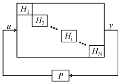
Figure 6: Linearized System Interconnection.

Since subsystems in the same class have identical models, they have identical $\mathcal{L}_{2}$-gains. Let $\gamma_{i}$ denote the $\mathcal{L}_{2}$-gain of each subsystem in class $i$, and let $\Gamma$ be a diagonal matrix with entries

$$\{\Gamma\}_{jj}=\gamma_{i}\ \text{ for }\ j\in O_{i}.$$ (35)

The following Proposition provides a small-gain criterion for the stability of the cell network around the steady state pattern.

Theorem V.1

Consider the network (2)-(3). The steady state pattern defined by (33) is locally asymptotically stable if

$$\rho(P\Gamma)<1,$$ (36)

where $\Gamma$ is as in (35).

Proof:

Since each linearized subsystem $H_{i}$, in (34), has bounded $\mathcal{L}_{2}$ gain, by the Bounded Real Lemma [22], we conclude that there exists a positive definite matrix $Q_{i}$ such that, for $V_{i}(z)=z^{T}Q_{i}z$, we have $\dot{V}_{i}(x^{i},u^{i})\leq\gamma_{i}^{2}u^{iT}u^{i}-y^{iT}y^{i}$. Let $D=diag\{d_{1},\ldots,d_{n}\}$, where $d_{i}$ is some positive constant, and let $V(x)=\sum_{i}d_{i}V_{i}$. We then obtain,

$$\dot{V}(x) = \sum_{i}d_{i}\dot{V}_{i}(x^{i},u^{i})$$ (37)

$$\leq U^{T}D\Gamma^{2}U-Y^{T}DY$$ (38)

$$= Y^{T}((\Gamma P)^{T}D(\Gamma P)-D)Y,$$ (39)

where $U=[(u^{1})^{T}\ldots(u^{N})^{T}]^{T}$, $Y=[(y^{1})^{T}\ldots(y^{N})^{T}]^{T}$, and the second equality follows from the fact that $U=PY$. If $\dot{V}(x)$ is negative semidefinite, we know from LaSalle’s Invariance Principle [23], and for linear systems ([24]), that every trajectory converges to the unobservable subspace of the system. Furthermore, under the same assumption, and since each $H_{i}$ is observable, we conclude that each trajectory must converge to the singleton $\{0\}$. Thus, the steady-state (33) is locally asymptotically stable, if there exists a positive diagonal matrix $D$ such that $D-(\Gamma P)^{T}D(\Gamma P)$ is positive definite. This is equivalent to the condition that $I-\Gamma P$ be a M-matrix, see [25, Theorem 2]. To finalize the proof, note that the spectra of $P\Gamma$ is the same as $\Gamma P$, and that the radial spectra assumption implies that $I-\Gamma P$ is a nonsingular M-matrix, see [26, Definition 6.1.2]. ∎

We now show that (36) is equivalent to $\rho(\overline{P}\overline{\Gamma})<1$, where

$$\overline{\Gamma}=diag\{\gamma_{1},\ldots,\gamma_{r}\}.$$ (40)

This result simplifies the verification of this small gain stability condition to the reduced system $S_{R}$ in (29) with interconnection matrix $\overline{P}$.

Lemma V.2

Consider an equitable partition $\pi$ of $\mathcal{G}$. Then,

$$\rho(P\Gamma)<1\Leftrightarrow\rho(\overline{P}\overline{\Gamma})<1,$$ (41)

where $\overline{P}$ is as in (9), and $\overline{\Gamma}$ is as in (40).

Proof:

To prove this statement we only need to show that

$$\rho(\overline{P}\overline{\Gamma})=\rho(P\Gamma).$$ (42)

First, note that $\overline{P}\overline{\Gamma}$ is a nonnegative irreducible matrix, by the Perron-Frobenius Theorem [26], we know that $r=\rho(\overline{P}\overline{\Gamma})>0$ is an eigenvalue of $\overline{P}\overline{\Gamma}$ with corresponding eigenvector $\overline{v}\gg 0$.
Claim: $r>0$ is also an eigenvalue of $P\Gamma$ with corresponding eigenvector $v$ such that entries $v_{i}=\overline{v}_{j}$ if $i\in O_{j}$.
According to this claim, we know that $v$ is a positive eigenvector. Therefore, by citing again the Perron-Frobenius Theorem, and since $P\Gamma$ is also a nonnegative irreducible matrix, we conclude that $v$ has to be the eigenvector associated with eigenvalue $r=\rho(P\Gamma)$.
To prove the claim, note that matrix $\Gamma$ is positive diagonal with repeated entries for vertices in the same class. Therefore, since the vertex partition is equitable for the scaled adjacency graph $P$, then it is also equitable when we consider a modified adjacency graph $P\Gamma$, i.e.,

$$\sum_{v\in O_{j}}p_{uv}\gamma_{jj}=\overline{p}_{ij}\gamma_{jj}\quad\forall u\in O_{i},$$ (43)

where $\overline{p}_{ij}$ is as defined in (9). From this observation we see that this claim is a generalization of the Lifting Proposition in [14], which holds not only for partitions obtained through an automorphism subgroup but also for any equitable partition. The proof of the claim follows similarly to the proof of the Lifting Proposition, with matrices $P\Gamma$ and $\overline{P}\overline{\Gamma}$ as in (43). ∎

Lemma V.2 leads to a simplification of the stability condition (36) in Theorem V.1.

Corollary V.3

Consider the network (2)-(3). The steady state pattern defined by (33) is locally asymptotically stable if

$$\rho(\overline{P}\overline{\Gamma})<1.$$ (44)

$\blacksquare$

V-C Special Case: Bipartite Graph

Let us consider the special case of a bipartite graph, with a partition $\pi$ consisting of two classes, chosen so that no two vertices in the same set are adjacent. As discussed before, in Example 1, the quotient matrix $\overline{P}$ is given by

$$\overline{P}=\left[\begin{array}[]{cc}0&1\\ 1&0\end{array}\right].$$ (45)

Therefore, the spectra of $\overline{P}\overline{\Gamma}$ is $\pm\sqrt{\gamma_{1}\gamma_{2}}$. The next result follows trivially from Corollary V.3.

Corollary V.4

Assume that the contact graph $\mathcal{G}$ of the cell network (2)-(3) is bipartite, and that there exists a steady state $u\in R^{N}$ such that $u_{i}=z_{1}$ if $i\in O_{1}$ and $u_{i}=z_{2}$ if $i\in O_{2}$, with $z_{1}\neq z_{2}\neq z^{*}$, as in Corollary III.3. Then, the steady state solution is locally asymptotically stable if

$$\gamma_{1}\gamma_{2}<1,$$ (46)

where $\gamma_{1}$ and $\gamma_{2}$ are the $\mathcal{L}_{2}$ gains of the linearized subsystems around $z_{1}$ and $z_{2}$, respectively. $\blacksquare$

In the particular case where the $\mathcal{L}_{2}$-gain is given by the dc-gain,

$$\gamma_{i}=-C^{i}(A^{i})^{-1}B^{i}=-T^{\prime}(z_{i}),$$ (47)

we see that the local asymptotic stability condition in (46) reduces to

$$T^{\prime}(z_{1})T^{\prime}(z_{2})<1.$$ (48)

The $\mathcal{L}_{2}$-gain is indeed equal to the dc-gain in the particular case where each subsystem (2) is input-output monotone [27], as assumed in [28]. We have thus recovered Theorem 2 in [28] which used (48) to prove the existence of stable checkerboard patterns.
Unlike the proof in [28], which relies heavily on monotonicity properties, here we have only assumed that the $\mathcal{L}_{2}$-gain is equal to the dc-gain.

VI Conclusions

In this paper we presented analytical results to predict steady-state patterns for large-scale lateral inhibition systems. We have shown that equitable partitions provide templates for steady state pattern candidates, as they identify invariant subspaces where the fate of cells in the same class is identical. We proved the existence of steady state patterns by relying on the static input-output model of each cell and the algebraic properties of the contact graph. One limitation in these results is the assumption that the reduced graph is bipartite. Therefore, the generalization to a larger class of graph partitions, that do not necessarily result in bipartite reduced graphs, needs to be investigated. Further results will also focus on the case where the cell model is multiple-input multiple-output, representing cell-to-cell inhibition signals that depend on more than one species.

Finally, we have analyzed the stability of steady state patterns by providing a decomposition into a representative subsystem $S_{R}$ and a transverse subsystem $S_{D}$. We also provide a small-gain stability type criterion, which relies only on the reduced order subsystem $S_{R}$ to guarantee stability of the steady state patterns.

References

- [1] S. Gilbert, Developmental Biology. Sinauer Associates, Inc., ninth ed., 2010.
- [2] L. Wolpert and C. Tickle, Principles of Development. Oxford University Press, fourth ed., 2011.
- [3] A. M. Turing, “The Chemical Basis of Morphogenesis,” Philosophical Transactions of the Royal Society of London. Series B, Biological Sciences, vol. 237, pp. 37–72, Aug. 1952.
- [4] A. Gierer and H. Meinhardt, “A theory of biological pattern formation.,” Biological Cybernetics, vol. 12, pp. 30–39, Dec. 1972.
- [5] R. Dillon, P. K. Maini, and H. G. Othmer, “Pattern formation in generalized turing systems,” Journal of Mathematical Biology, vol. 32, pp. 345–393, 1994.
- [6] J. D. Murray, Mathematical Biology II: Spatial Models and Biomedical Applications, vol. 18 of Interdisciplinary Applied Mathematics. Springer New York, 2003.
- [7] D. Sprinzak, A. Lakhanpal, L. LeBon, L. A. Santat, M. E. Fontes, G. A. Anderson, J. Garcia-Ojalvo, and M. B. Elowitz, “Cis-interactions between notch and delta generate mutually exclusive signalling states,” Nature, vol. 465, pp. 86–90, 05 2010.
- [8] J. Collier, N. Monk, P. Maini, and J. Lewis, “Pattern formation by lateral inhibition with feedback: a mathematical model of delta-notch intercellular signalling.,” Journal of theoretical biology, vol. 183, pp. 429–446, 12 1996.
- [9] D. Sprinzak, A. Lakhanpal, L. LeBon, J. Garcia-Ojalvo, and M. B. Elowitz, “Mutual Inactivation of Notch Receptors and Ligands Facilitates Developmental Patterning,” PLoS Comput Biol, vol. 7, p. e1002069, June 2011.
- [10] M. Arcak, “On biological pattern formation by contact inhibition,” in 2012 American Control Conference, 2012.
- [11] H. Smith, Monotone Dynamical Systems: An Introduction to the Theory of Competitive and Cooperative Systems. Mathematical Surveys and Monographs, American Mathematical Society, 1995.
- [12] I. Stewart, M. Golubitsky, and M. Pivato, “Symmetry groupoids and patterns of synchrony in coupled cell networks,” SIAM J. Appl. Dynam. Sys, vol. 2, pp. 609–646, 2003.
- [13] M. Golubitsky and I. Stewart, “Nonlinear dynamics of networks: the groupoid formalism,” Bulletin of the American Mathematical Society, vol. 43, pp. 305–364, 2006.
- [14] S. P. Boyd, P. Diaconis, P. A. Parrilo, and L. Xiao, “Symmetry analysis of reversible markov chains.,” Internet Mathematics, vol. 2, no. 1, pp. 31–71, 2005.
- [15] S. Boyd, P. Diaconis, P. Parrilo, and L. Xiao, “Fastest mixing markov chain on graphs with symmetries,” SIAM J. on Optimization, vol. 20, pp. 792–819, June 2009.
- [16] K. Gatermann and P. A. Parrilo, “Symmetry groups, semidefinite programs, and sums of squares,” Journal of Pure and Applied Algebra, vol. 192, no. 1–3, pp. 95 – 128, 2004.
- [17] A. Rahmani, M. Ji, M. Mesbahi, and M. Egerstedt, “Controllability of multi-agent systems from a graph-theoretic perspective,” SIAM J. Control Optim., vol. 48, pp. 162–186, Feb. 2009.
- [18] C. Godsil and G. Royle, Algebraic Graph Theory. Springer, Apr. 2001.
- [19] The GAP Group, GAP – Groups, Algorithms, and Programming, Version 4.4.12, 2008.
- [20] Y. Wang and M. Golubitsky, “Two-colour patterns of synchrony in lattice dynamical systems,” Nonlinearity, vol. 18, no. 2, p. 631, 2005.
- [21] D. Cvetković, M. Doob, and H. Sachs, Spectra of graphs: theory and application. Pure and applied mathematics, Academic Press, 1980.
- [22] J. Doyle, K. Glover, P. Khargonekar, and B. Francis, “State-space solutions to standard h2 and h infin; control problems,” Automatic Control, IEEE Transactions on, vol. 34, pp. 831 –847, aug 1989.
- [23] H. Khalil, Nonlinear Systems (3rd Edition). Englewood Cliffs, NJ: Prentice Hall, 2002.
- [24] W. J. Rugh, Linear systems theory. Englewood Cliffs, N.J.: Prentice Hall, 2nd ed., 1993.
- [25] M. Araki, “Application of m-matrices to the stability problems of composite dynamical systems,” Journal of Mathematical Analysis and Applications, vol. 52, no. 2, pp. 309 – 321, 1975.
- [26] A. Berman and R. J. Plemmons, Nonnegative Matrices in the Mathematical Sciences. Philadelphia, PA: Society for Industrial and Applied Mathematics (SIAM), 1994. (revised reprint of the 1979 original).
- [27] D. Angeli and E. Sontag, “Multi-stability in monotone input/output systems,” Systems & Control Letters, vol. 51, pp. 185–202, Mar. 2004.
- [28] M. Arcak, “Pattern formation by lateral inhibition in large-scale networks of cells,” Automatic Control, IEEE Transactions on, vol. to appear, May 2013.