Filters for High Rate Pulse Processing

Abstract

We introduce a filter-construction method for pulse processing that differs in two respects from that in standard optimal filtering, in which the average pulse shape and noise-power spectral density are combined to create a convolution filter for estimating pulse heights. First, the proposed filters are computed in the time domain, to avoid periodicity artifacts of the discrete Fourier transform, and second, orthogonality constraints are imposed on the filters, to reduce the filtering procedure’s sensitivity to unknown baseline height and pulse tails. We analyze the proposed filters, predicting energy resolution under several scenarios, and apply the filters to high-rate pulse data from gamma-rays measured by a transition-edge-sensor microcalorimeter.

Keywords

baseline insensitivity, energy resolution, optimal filtering, pulse pile-up, pulse tail insensitivity

PACS numbers

07.20.Mc, 07.05.Kf, 84.30.Sk.

U.S. government publication

Not subject to copyright.

The extraction of physical quantities from noisy data streams is ubiquitous in the physical sciences. Examples include the determination of photon and particle energies or incidence times in nuclear and particle physics. Raw data records are invariably filtered to extract the quantity of interest with the highest signal-to-noise, and extensive effort has gone into filter development. One important example is so-called “optimal filtering,” for isolated pulses with amplitude proportional to photon energy. Filters constructed from the average pulse shape and the noise power spectral density are convolved with pulse records to estimate pulse amplitudes Szymkowiak et al. (1993). This filter is widely used in X-ray astrophysics Eckart et al. (2012) and direct searches for weakly interacting dark matter Ahmed et al. (2011).

Here, we propose and demonstrate a novel method for optimal-filter construction for pulse processing. The previous optimal filter is shown to be an example of a much larger class of filters that have new and useful properties. For example, optimal filters can be constructed that are orthogonal to exponential tails of prior pulses, prompted by the need to cope with high-rate pulse data. Many applications of high-resolution photon spectroscopy require very large photon counts for accurate characterization of an absorption or emission spectrum across a broad energy band. For example, isotopic analysis of nuclear materials for treaty verification requires approximately $10^{9}$ photons in a spectrum between 60 keV and 260 keV to achieve uncertainty of $10^{-3}$ Jethava et al. (2009). Low-temperature detectors can reach this goal, within limited collection periods, only through large arrays of elements operating at high photon count rates per element. Consequently, operation at high count rates is an active topic of research Tan et al. (2008, 2009, 2011); Alpert et al. (2012).

The new framework departs from prior algorithms in two respects: (1) noise autocovariance is used in place of its mathematical dual, the noise power spectral density, to avoid the discrete Fourier transform (DFT) and enable the construction to be entirely in the time domain; and (2) the filter optimization is subject to explicit constraints beyond maximization of signal-to-noise ratio for isolated pulses, including for the filter length, orthogonality to constants, and orthogonality to exponentials of one or more decay rates. (The method is related to constrained optimization in some other contexts. For example, a similar approach has recently been developed for designing matched filters for wavefront sensing Gilles and Ellerbroek (2008).) Orthogonality to exponentials can reduce or eliminate sensitivity to tails of prior pulses. With these additional constraints imposed, the filters suffer some loss of sensitivity for isolated pulses compared to filters optimized for that case, but they compensate by retaining resolution with piled-up pulses and by avoiding DFT artifacts, including artificial periodicity.

Processing procedure.

Estimation of pulse amplitudes under standard filtering Szymkowiak et al. (1993); Moseley et al. (1988) is optimized for isolated pulses. Each pulse is convolved with a filter and the maximum of the convolution (or a smoothed maximum as provided by a quadratic polynomial fit to several values near the maximum) provides an estimate of the pulse amplitude. The filter, in principle, is constructed to minimize the variance of this estimate, given a known pulse shape and known noise power spectrum.

Continuous time model.

We assume a signal $f$ consists of a pair of pulses sitting on a baseline

$$f(t)=a_{0}s(t-t_{0})+a_{1}s(t-t_{1})+b,$$

where $s$ is the pulse shape, $a_{0}$ and $a_{1}$ are the pulse amplitudes, $t_{0}$ and $t_{1}$ are the pulse arrival times, with $t_{0}<t_{1}$, and $b$ is the baseline. A noisy signal consists of signal plus noise, $m(t)=f(t)+\eta(t),$ where the noise $\eta$ is assumed to be a realization of a stationary stochastic process with a mean of zero and autocovariance

$$R_{\eta}(\tau)=\int_{-\infty}^{\infty}\eta(t)\eta(t+\tau)dt.$$

Discrete time model.

The measurement apparatus obtains an approximation $m_{i}$ of $m(i\Delta)$ for $i$ an integer, where $\Delta$ is the sample time spacing, as a convolution of $m$ with a response function

$$m_{i}=\int_{-\infty}^{\infty}m(i\Delta-t)w(t)dt,$$

where $w$ is an approximate $\delta$-function centered at the origin with unit integral. We define $f_{i},$ $s_{i},$ and $\eta_{i}$ analogously. Our measurement model is then

$$m_{i} =f_{i}+\eta_{i}$$

$$=a_{0}s_{i-i_{0}}+a_{1}s_{i-i_{1}}+b+\eta_{i}.$$ (1)

In this approximate model, arrival times $t_{0}=i_{0}\Delta,\;t_{1}=i_{1}\Delta$ are assumed aligned with the samples, and known, to avoid interpolation issues. The pulse shape $s=(s_{0},\ldots,s_{n},\ldots)^{t}$ is approximated by averaging many pulses to obtain the estimate $\hat{s}=(\hat{s}_{0},\ldots,\hat{s}_{n},\ldots)^{t}$, normalized so $\max\hat{s}=1$, and the noise autocovariance $r=(r_{0},\ldots,r_{n},\ldots)^{t}$, given by the expectation

$$r_{k}=\mathbb{E}\left[\eta_{i}\eta_{i+k}\right]-\mathbb{E}\left[\eta_{i}\right]^{2}=\mathbb{E}\left[\eta_{i}\eta_{i+k}\right],$$ (2)

is approximated by averaging products of pulse-free samples of the sensor output to obtain the estimate $\hat{r}=(\hat{r}_{0},\ldots,\hat{r}_{n},\ldots)^{t}$.

Amplitude estimation.

The standard procedure assumes $a_{0}=0$, computes the discrete convolution

$$(q\star m)_{i}=\sum_{j=0}^{n-1}q_{j}m_{i-j}$$

of a given filter $q=(q_{0},\ldots,q_{n-1})^{t}$ with $\ldots,m_{-1},m_{0},m_{1},\ldots,$ the discrete convolution of $q$ with $\ldots,\hat{s}_{-1},\hat{s}_{0},\hat{s}_{1},\ldots,$ where $\hat{s}_{i}=0$ for $i<0,$ and estimates $a_{1}$ as the ratio of their maximums

$$\hat{a}_{1}=\frac{\max_{i}(q\star m)_{i}}{\max_{i}(q\star\hat{s})_{i}}.$$ (3)

Estimate mean and variance.

We seek the mean and variance of the amplitude estimate $\hat{a}_{1}.$ We have

$$\mathbb{E}\left[(q\star m)_{i}\right]=a_{0}\cdot(q\star s)_{i-i_{0}}+a_{1}\cdot(q\star s)_{i-i_{1}}+b\sum_{j=0}^{n-1}q_{j}.$$ (4)

We define $\bar{\imath}$ so that $(q\star s)_{\bar{\imath}}=\max_{i}(q\star s)_{i}.$ Under assumptions of orthogonality to the prior tail and to constants,

$$(q\star s)_{\bar{\imath}+i_{1}-i_{0}}=0=\sum_{j=0}^{n-1}q_{j},$$ (5)

we have

$$\mathbb{E}\left[\hat{a}_{1}\right] =\frac{\mathbb{E}\left[\max_{i}(q\star m)_{i}\right]}{\max_{i}(q\star\hat{s})_{i}}$$

$$\approx\frac{\max_{i}\mathbb{E}\left[(q\star m)_{i}\right]}{\max_{i}(q\star\hat{s})_{i}}\approx\frac{a_{1}\cdot(q\star s)_{\bar{\imath}}}{(q\star\hat{s})_{\bar{\imath}}}\approx a_{1},$$ (6)

where the approximations are equalities under somewhat restrictive conditions.

Toward a variance estimate,

$$\mathbb{E}\left[m_{i-j}m_{i-k}\right]=\left(a_{0}s_{i-i_{0}-j}+a_{1}s_{i-i_{1}-j}+b\right)\\ \times\left(a_{0}s_{i-i_{0}-k}+a_{1}s_{i-i_{1}-k}+b\right)+r_{j-k},$$

where $r_{j-k}$ is the noise autocovariance of (2). Now

$${\rm Var}\left[\hat{a}_{1}\right] =\mathbb{E}\big{[}{\hat{a}_{1}}^{\;2}\big{]}-\mathbb{E}\left[\hat{a}_{1}\right]^{2}$$

$$=\frac{\mathbb{E}\big{[}\max_{i}(q\star m)_{i}^{\;2}\big{]}-\mathbb{E}\left[\max_{i}(q\star m)_{i}\right]^{2}}{\max_{i}(q\star\hat{s})_{i}^{\;2}}$$

$$\approx\frac{\max_{i}\mathbb{E}\big{[}(q\star m)_{i}^{\;2}\big{]}-\max_{i}\mathbb{E}\left[(q\star m)_{i}\right]^{2}}{\max_{i}(q\star\hat{s})_{i}^{\;2}}$$

$$=\frac{q^{t}Rq}{[q^{t}\overline{s}]^{2}}\approx\frac{q^{t}\hat{R}q}{[q^{t}\overline{s}]^{2}}\stackrel{{\scriptstyle\mathrm{def}}}{{=}}\hat{\rm V}{\rm ar}\left[\hat{a}_{1}\right],$$ (7)

where the variance estimate $\hat{\rm V}{\rm ar}\big{[}\hat{a}_{1}\big{]}$ is defined to be the last expression, $\hat{R}$ is the $n\times n$ estimated covariance matrix with $\hat{R}_{jk}=\hat{r}_{j-k}=\hat{r}_{|j-k|},$ and $\overline{s}=(\hat{s}_{i},\hat{s}_{i-1},\ldots,\hat{s}_{i-n+1})^{t}$ is the length $n$ segment from $\hat{s}$ with $q^{t}\overline{s}=\max_{i}(q\star\hat{s})_{i}$.

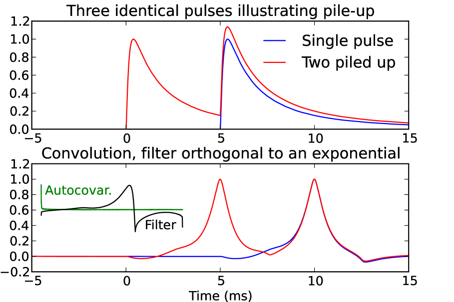
Figure 1: (color) Two scenarios, one with pile-up, are shown (top). From the pulse shape and noise autocovariance, a filter orthogonal to an exponential of tail decay, $\tau=3.2$ ms, is computed (inset, separate vertical scales). Convolution of the filter with the signal yields peaks of essentially constant height (bottom) and nearly eliminates pile-up dependence.

Table 1: Dataset summary for four photon count rates. Sample spacing was 2.56 $\mu$s, full stream data were kept, and records were later formed, including for two lengths shown. Discards resulted from insufficient time between triggered pulses, signal drops below baseline, and rises in pre-trigger or post-peak attributed to (untriggered) nuisance pulses.

Dataset	1	2	3	4
Duration (s)	4249.50	3096.93	3182.13	4583.17
Pulses triggered	5496	6581	17872	60267
Rate (Hz)	1.29	2.13	5.62	13.15
Records: 10.24 ms with 5.12 ms pre-trigger
Discards:
pulse starts ($>$1)	143	201	1088	7610
SQUID unlock	42	92	585	3648
early peak	22	17	62	167
pre-trigger rise	8	21	93	368
post-peak rise	5	13	65	631
97 keV (raw height)	1095	1286	3213	9607
Records: 25.60 ms with 6.40 ms pre-trigger
Discards:
pulse starts ($>$1)	243	387	2463	17266
SQUID unlock	40	90	537	2985
early peak	19	17	58	138
pre-trigger rise	8	23	105	606
post-peak rise	19	36	223	1325
97 keV (raw height)	1067	1228	2938	7565

Filter optimization.

This expression for the variance of the amplitude estimate enables us to design filters that minimize the estimated variance. $\hat{\rm V}{\rm ar}\big{[}\hat{a}_{1}\big{]}$ is minimized at a stationary point of the Lagrange function,

$$\Lambda(q,\lambda)=q^{t}\hat{R}q-\lambda\left[q^{t}\overline{s}-1,\right]$$

where $\lambda$ is a Lagrange multiplier to ensure that the scale of $q$ satisfies $q^{t}\overline{s}=1=\max\overline{s}.$ Setting the partial derivatives of $\Lambda$ to zero and solving gives

$$q=\frac{\hat{R}^{-1}\overline{s}}{\overline{s}^{t}\hat{R}^{-1}\overline{s}},\qquad\hat{\rm V}{\rm ar}\big{[}\hat{a}_{1}\big{]}=\left[\overline{s}^{t}\hat{R}^{-1}\overline{s}\right]^{-1}.$$ (8)

This solution depends on the choice, made above tacitly, of the length $n$ of the convolution filter $q$.

Extending beyond the prescription above, we optimize subject to stipulated constraints. Orthogonality to constants or exponentials of particular decay rates can be imposed by revising the Lagrange function. For orthogonality to $k$ vectors $V=\left[v_{1}\cdots v_{k}\right],$

$$\Lambda(q,\lambda,\gamma)=q^{t}\hat{R}q-\lambda\left[q^{t}\overline{s}-1\right]-q^{t}V\gamma,$$

where $\gamma=(\gamma_{1},\ldots,\gamma_{k})^{t}$ are $k$ additional Lagrange multipliers. The solution is

$$q=\hat{R}^{-1}\overline{V}\left(\overline{V}^{t}\hat{R}^{-1}\overline{V}\right)^{-1}e_{1},\qquad\hat{\rm V}{\rm ar}\big{[}\hat{a}_{1}\big{]}=q^{t}\hat{R}q,$$ (9)

where $\overline{V}=[\overline{s}\;v_{1}\cdots v_{k}]$ and $e_{1}=(1,0,\ldots,0)^{t}$ is of length $k+1.$

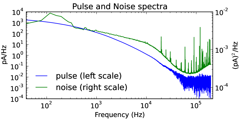
Figure 2: (color) Pulse spectrum is the absolute value of the discrete Fourier transform (DFT) of the average of pulses, near 97.431 keV line, from the highest-rate dataset. The noise spectrum is the average of the square of absolute value of DFT of pulse-free records of TES output. Records are 25.6 ms.

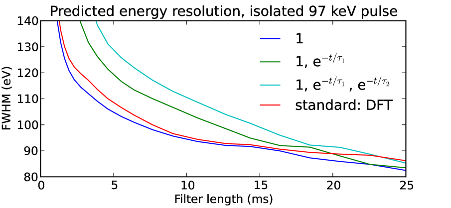
Figure 3: (color) Predicted resolution on an isolated pulse of four filters is shown. The filters, determined from average pulse shape and noise autocovariance (Fig. 2), include the standard DFT-computed filter with lowest frequency bin set to zero Doriese et al. (2009) and proposed filters orthogonal to constants and zero, one, or two exponentials ($\tau_{1}=6.0$ ms, $\tau_{2}=1.5$ ms).

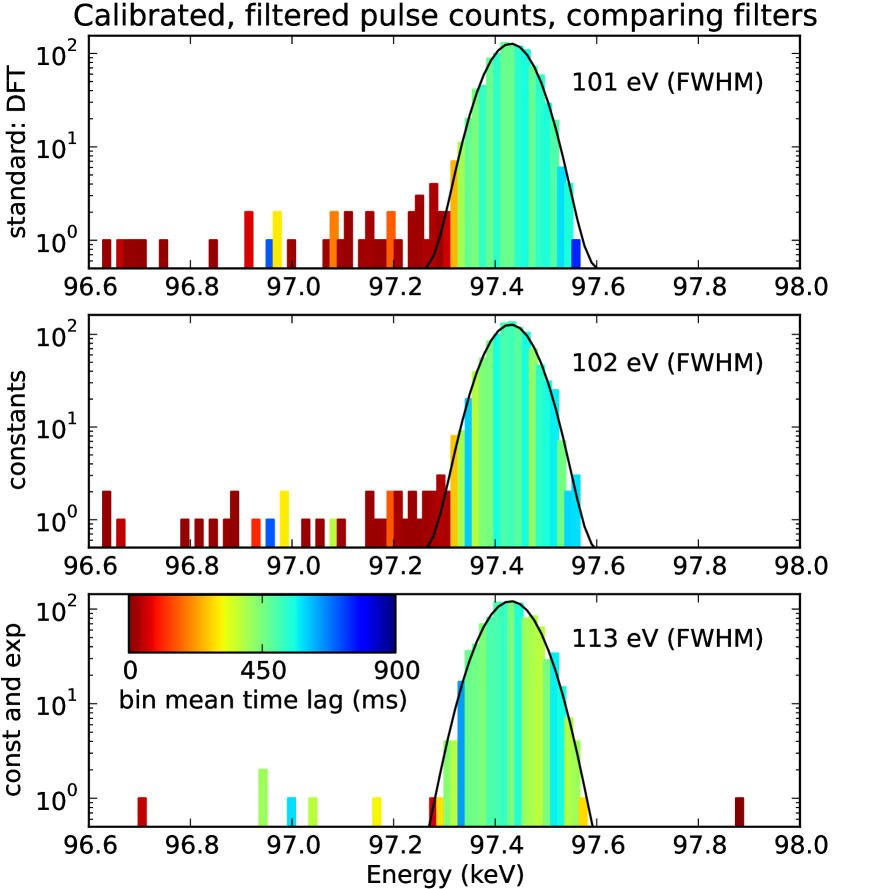
Figure 4: (color) Energy histograms near the 97.431 keV line, from the 2.13 Hz dataset with 10.24 ms record length, are shown for the standard filter, the proposed filter orthogonal to constants, and the proposed filter orthogonal to constants and exponentials ($\tau=6$ ms). Color denotes the pulse arrival time lag since the previous pulse, averaged over the histogram bin, and illustrates that filtering errors, concentrated in heavily piled-up pulses, are nearly eliminated by the filter orthogonal to exponentials.

Orthogonality to exponentials of a particular decay time constant enables filters to be less sensitive to tails of prior pulses. Fig. 1 illustrates the principle of these filters. Avoidance of the DFT, with an increase in filter computation cost that is very mild for filter lengths up to $n\approx 10^{4},$ avoids false assumptions of signal and noise periodicity and yields nonperiodic filters.

Experiment.

Measurements were taken at NIST of photons from a ¹⁵³Gd source with a single transition-edge-sensor (TES) microcalorimeter Bennett et al. (2012), at varied count rates (1.29, 2.13, 5.62, and 13.15 Hz), by placing the source at four different distances from the detector. Essentially all pulses were filtered; no attempt was made to selectively discard pulses to improve the energy resolution. In extraction of pulse records from the data streams, pulses were lost principally due to onset within the prior pulse record and to occasional SQUID mode unlock. Statistics for these measurements are summarized in Table 1. The following analysis focuses on pulses near the 97.431 keV gamma-ray emission line of ¹⁵³Gd.

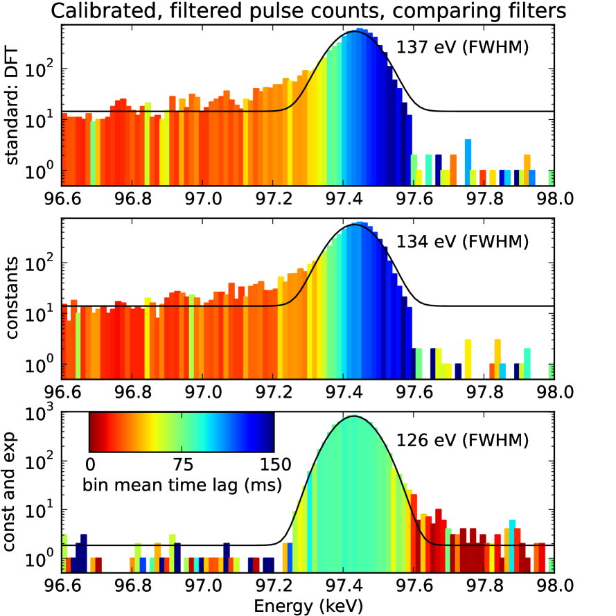
Figure 5: (color) Energy histograms as in Fig. 4, except from 13.15 Hz dataset. At this higher rate, the errors of the first two filters are much more significant, as is the improvement offered by the third.

The noise spectrum and, for comparison, the spectrum of the average pulse are plotted in Fig. 2. The noise spectrum and the DFT of the average pulse are used to compute the standard filter. The autocovariance and the average pulse (shown above in Fig. 1) are used to compute the proposed filters and the predicted energy resolution of each. Fig. 3 shows predicted resolution versus filter length for the proposed filters and the standard DFT-computed optimal filter, with the lowest frequency bin set to zero to reduce sensitivity to baseline drift. The standard filter and the proposed filter orthogonal to constants would agree, absent discretization and periodicity artifacts due to the DFT. This calculation is for isolated pulses; for piled-up pulses these two filters suffer bias problems that are significantly reduced by the filters orthogonal to exponentials. The filter orthogonal to two exponentials, however, due to the additional constraint, suffers significant loss of sensitivity at short to moderate filter lengths, and is not considered further here.

The performance of the other three filters is compared on measured pulses, and histograms near the 97.431 keV line are plotted for two different pulse rates in Fig. 4 and Fig. 5. Each histogram was fit with a Gaussian plus a constant to determine the energy resolution. The histogram bins are colored based on the pulse arrival-time lag from the previous pulse, averaged over the bin, demonstrating that errors in processing are due mainly to closely piled-up pulses and are significantly ameliorated by the proposed filters orthogonal to exponentials. This effect is pronounced at the higher pulse rate, yielding much-enhanced peak height and reduced leakage for the filter orthogonal to exponentials.

In Fig. 6 the output pulse rate, for the energy range $97.431\pm 0.100$ keV, and energy resolution are compared for all four input count rates and the three types of filter, for both short and long pulse records. At the highest rate and for short pulse records, the filter orthogonal to both constants and exponentials ($\tau=6$ ms) offers 45 % higher output rate than the standard DFT-computed filter and 40 % higher than the filter orthogonal to constants alone, at better energy resolution than either one.

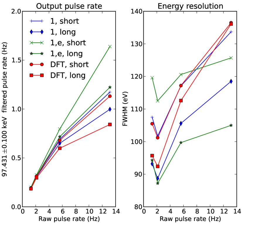
Figure 6: (color) The output pulse rate and energy resolution are compared across input count rates and three filter types ($\tau=6$ ms), for both short (10.24 ms) and long (25.60 ms) pulse records. We note that the maximum output pulse rate is considerably lower than the corresponding raw pulse rate, because many raw pulses are due to spectral features other than the 97.431 keV line.

One important issue regarding the filters orthogonal to exponentials concerns their performance sensitivity to the choice of decay time constant $\tau$. The average pulse, for the TES microcalorimeter tested, was well-approximated over a 25.6 ms record by a linear combination of four exponentials, with decay time constants $\tau=$ 0.018 ms, 0.144 ms, 0.963 ms, and 2.514 ms. If just the tail is fit, however, the constants increase considerably. It is evident, therefore, that no single decay rate is optimal for all arrival-time lags. Nevertheless, for the full set of Poisson-distributed arrival time lags, the performance of the filters is only mildly sensitive to the choice of time constant. For the highest-rate data with short records, over the range $\tau=3,\ldots,10$ ms, the $97.431\pm 0.100$ keV output pulse rate varied as $1.568\pm 0.044$ Hz (mean and one standard deviation) and the energy resolution varied as $128.3\pm 3.2$ eV, as compared with the $\tau=6$ ms values of 1.640 Hz and 125.7 eV.

Summary.

The proposed filter construction method, differing from the standard procedure by being computed in the time domain and enabling filter optimization subject to explicit length and orthogonality constraints, assumes linear superposition of pulses and simple exponential decay of pulse tails. Although these assumptions are satisfied rather imperfectly for the TES microcalorimeter tested, the method yields notable improvement over standard filtering. Our tests also point to additional, more specialized options, such as filters optimized for a particular interval of arrival time lags since the previous pulse. Such filters fit easily within this framework and underline that the new approach has implications for pulse processing in a broad range of applications.

We gratefully acknowledge support from the NIST Innovations in Measurement Science program, the DOE Office of Nuclear Nonproliferation Research and Development, and the DOE Office of Nuclear Energy.

References

- Szymkowiak et al. (1993) A. E. Szymkowiak, R. L. Kelley, S. H. Moseley, and C. K. Stahle, J. Low Temp. Phys. 93, 281 (1993).
- Eckart et al. (2012) M. E. Eckart, J. S. Adams, C. N. Bailey, S. R. Bandler, S. E. Busch, J. A. Chervenak, F. M. Finkbeiner, R. L. Kelley, C. A. Kilbourne, F. S. Porter, J. P. Porst, J. E. Sadleir, and S. J. Smith, Journal of Low Temperature Physics 167, 732 (2012).
- Ahmed et al. (2011) Z. Ahmed, D. Akerib, S. Arrenberg, et al., Physical Review Letters 106, 131302 (2011).
- Jethava et al. (2009) N. Jethava, J. N. Ullom, D. A. Bennett, W. B. Doriese, J. A. Beall, G. C. Hilton, R. D. Horansky, K. D. Irwin, E. Sassi, L. R. Vale, M. K. Bacrania, A. S. Hoover, P. J. Karpius, M. W. Rabin, C. R. Rudy, and D. T. Vo, IEEE Transactions on Applied Superconductivity 19, 536 (2009).
- Tan et al. (2008) H. Tan, D. Breus, W. Hennig, K. Sabourov, W. K. Warburton, W. B. Doriese, J. N. Ullom, M. K. Bacrania, A. S. Hoover, and M. W. Rabin, IEEE Nucl. Sci. Symp. Conf. Record, 1130 (2008).
- Tan et al. (2009) H. Tan, D. Breus, W. Hennig, K. Sabourov, J. W. Collins, W. K. Warburton, W. B. Doriese, J. N. Ullom, M. K. Bacrania, A. S. Hoover, and M. W. Rabin, AIP Conf. Proc. (American Institute of Physics) 1185, 294 (2009).
- Tan et al. (2011) H. Tan, W. Hennig, W. K. Warburton, W. B. Doriese, and C. A. Kilbourne, IEEE Trans. Applied Superconductivity 21, 276 (2011).
- Alpert et al. (2012) B. K. Alpert, W. B. Doriese, J. W. Fowler, and J. N. Ullom, Journal of Low Temperature Physics 167, 582 (2012).
- Gilles and Ellerbroek (2008) L. Gilles and B. L. Ellerbroek, Optics Letters 33, 1159 (2008).
- Moseley et al. (1988) S. H. Moseley, R. L. Kelley, R. J. Schoelkopf, A. E. Szymkowiak, D. McCammon, and J. Zhang, IEEE Trans. Nucl. Science 35, 59 (1988).
- Doriese et al. (2009) W. B. Doriese, J. S. Adams, G. C. Hilton, K. D. Irwin, C. A. Kilbourne, F. J. Schima, and J. N. Ullom, in Low Temperature Detectors LTD 13, AIP Conference Proceedings, Vol. 1185, edited by B. Cabrera, A. Miller, and B. Young (2009) pp. 450–453.
- Bennett et al. (2012) D. A. Bennett, R. D. Horansky, D. R. Schmidt, A. S. Hoover, R. Winkler, B. K. Alpert, J. A. Beall, W. B. Doriese, J. W. Fowler, C. P. Fitzgerald, G. C. Hilton, K. D. Irwin, V. Kotsubo, J. A. B. Mates, G. C. O’Neil, M. W. Rabin, C. D. Reintsema, F. J. Schima, D. S. Swetz, L. R. Vale, and J. N. Ullom, Review of Scientific Instruments 83, 093113 (2012).