Abstract

Physical properties of the Cornell potential in the complex-mass scheme are investigated. Two exact asymptotic solutions of relativistic wave equation for the coulombic and linear components of the potential are used to derive the resonance complex-mass formula. The centered masses and total widths of the $\rho$-family resonances are calculated.
Pacs: 11.10.St; 12.39.Pn; 12.40.Nn; 12.40.Yx
Keywords: meson, quark, bound state, resonance, complex mass, width

1. Introduction

Resonance is the tendency of a system to oscillate at a greater amplitude at some frequencies. Most particles listed in the Particle Data Group tables [2] are unstable. A thorough understanding of the physics summarized by the PDG is related to the concept of a resonance.

There are great amount and variety of experimental data and the different approaches used to extract the intrinsic properties of the resonances. In Quantum Mechanics and Quantum Field Theory resonances may appear in similar circumstances to classical physics. They can also be thought of as unstable particles with the particle’s complex energy poles in the scattering amplitude.

As known, operators in QM are Hermitian and the corresponding eigenvalues are real. However, in scattering experiment, the wave function requires another boundary condition (different from bound state’s), that is why the complex energy is required [3, 4].

It was in 1939 that Siegert introduced the concept of a purely outgoing wave belonging to the complex eigenvalue $\mathcal{E}_{n}=E_{n}-i\Gamma_{n}/2$ as an appropriate tool in the studying of resonances [5]. This complex eigenvalue also corresponds to a first-order pole of the S-matrix [6].

In elastic and inelastic scattering experiments the resonances are associated with the scattering particle and the target [7]. In such case the energy decreases exponentially with the time so that the damping constant $\Gamma$ is a measure of the lifetime, $\tau=h/\Gamma$, of the oscillation.

Resonances in QFT are described by the complex-mass poles of the scattering matrix [4]. Resonance is present as transient oscillations associated with metastable states of a system which has sufficient energy to break up into two or more subsystems. The masses of intermediate particles develop imaginary masses from loop corrections [8]. In this case, the probability density comes from the particle’s propagator, with the complex mass,

$$\mathcal{M}=M-i\Gamma/2.$$ (1)

This formula is related to the particle’s decay rate by the optical theorem [4, 9].

The hadronic resonances are never observed directly but through their decay channels; this causes problems with their definition. There is the lack of a precise definition of what is meant by mass and width of resonance. Comprehensive definitions of the centered mass and width of resonances require further investigations [10].

Fundamentals of scattering theory and strict mathematical definition of resonances in QM was considered in [11]. The rigorous QM definition of a resonance requires determining the pole position in the second Riemann sheet of the analytically continued partial-wave scattering amplitude in the complex Mandelstam $s$ variable plane [12].

Resonances are defined as the poles of the meromorphic continuation of the cut-off resolvent, which are shown to be the same as the poles of the meromorphically continued S-matrix. This definition has the advantage of being quite universal regarding the pole position, but can only be applied if the amplitude can be analytically continued in a reliable way.

In particle physics resonances arise as unstable intermediate states with complex masses. The advantage of analyzing a system in the complex plane has important features such as a simpler and more general framework. Complex numbers allow to get more than what we insert. The complex-mass scheme provides a consistent framework for dealing with unstable particles and has been successfully applied to various loop calculations [8].

In traditional approach to investigate resonances one deals with the scattering theory, exploring the properties of S-matrix and partial amplitudes. In this work, in contrast to the usual analysis, we consider mesonic resonances to be the quasi-bound states of a hadron constituents. We solve the bound-state problem in the potential approach and analyze the mass spectrum generated from solution of the relativistic wave equation for the Cornell potential. We show, that two asymptotic components of the potential, the coulombic term and linear one yield the complex masses of resonances. This results in the complex-mass formula for the resonances that allows to calculate in unified way their centered masses and total widths.

2. The universal mass formula

In perturbative QCD, as in QED the essential interaction at small distances is instantaneous coulombic one-gluon exchange (OGE); in QCD, it is $qq$, $qg$, or $gg$ Coulomb scattering [13]. Therefore, one expects from OGE a Coulomb-like contribution to the potential, i.e., $V_{S}(r)\propto-\alpha_{s}/r$ at $r\rightarrow 0$.

For large distances, in order to be able to describe confinement, the potential has to rise to infinity. From lattice-gauge-theory computations [14] follows that this rise is an approximately linear, i.e., $V_{L}(r)\simeq\sigma r+$const for large $r$, where $\sigma\simeq 0.15$ GeV² is the string tension. These two contributions by simple summation lead to the famous Cornell $q\bar{q}$ potential [14, 15],

$$V(r)=V_{S}(r)+V_{L}(r)\equiv-\frac{4}{3}\frac{\alpha_{s}}{r}+\sigma r;$$ (2)

its parameters are directly related to basic physical quantities noted above. All phenomenologically acceptable QCD-inspired potentials are only variations around this potential.

This potential is one of the most popular in hadron physics and incorporates in clear form the basic features of the strong interaction. In hadron physics, the nature of the potential is very important. There are normalizable solutions for scalarlike potentials, but not for vectorlike. The effective interaction has to be Lorentz-scalar in order to confine quarks and gluons [16]. In our consideration, we take the potential (2) to be Lorentz-scalar.

It is hard to find an analytic solution of known relativistic wave equations for the potential (2). This aim can be achieved with the use of the semi-classical wave equation [17]. An important feature of this equation is that, for two and more turning-point problems, it can be solved exactly by the conventional WKB method [17, 18].

Our aim is to find in analytic form the energy/mass eigenvalues for the potential (2). This is not easy task even for the quasiclassical method. This is why, using the two-point Padé approximant, we joined two exact solutions obtained separately for the short-distance coulombic part, $V_{S}(r)$, and long-distance one, $V_{L}(r)$, of the Cornell potential. As a result we obtained the interpolating mass formula [19, 20, 21, 22],

$$M_{n}^{2}=4\left[2\sigma\tilde{N}-\left(\frac{\tilde{\alpha}m}{N}\right)^{2}+m^{2}-2\tilde{\alpha}\sigma\right],$$ (3)

where $\tilde{\alpha}=(4/3)\alpha_{s}$, $\tilde{N}=N+n_{r}+1/2$, $N=n_{r}+J+1$ and $m$ is the constituent quark mass. The simple mass formula (3) describes equally well the mass spectra of all $q\bar{q}$ and $Q\bar{Q}$ mesons ranging from the $u\bar{d}$ ($d\bar{d}$, $u\bar{u}$, $s\bar{s}$) states up to the heaviest known $b\bar{b}$ systems [21, 22].

The obtained from Eq. (3) “saturating” Regge trajectories [21, 22] were applied with success to Compton scattering, vector meson photoproduction and the partonic structure of the nucleon [23], the photoproduction of vector mesons that provide an excellent simultaneous description of the high and low $-t$ behavior of the $\gamma\,p\rightarrow p\,\rho$, $\omega$, $\phi$ cross sections [24], to interpretation of the space-time structure of hard scattering processes [25], given an appropriate choice of the relevant coupling constants (JML-model) [26, 27]. It was shown that the hard-scattering mechanism is incorporated in an effective way by using the “saturated” Regge trajectories that are independent of $t$ at large momentum transfers [22, 21, 28, 29].

The universal formula (3) has been used to calculate the glueball masses and Regge trajectories including the Pomeron [19, 20]. It appears to be successful in many applications and can be justified with the use of the complex-mass scheme.

3. The complex-mass eigenvalues

Resonances are complex values and can be described by complex numbers. These numbers are important even if one wants to find real solutions of a problem. Using complex numbers, we are getting more than what we insert. Remind the important properties of complex numbers such as the fundamental theorem of algebra, i.e., the existence of $n$ roots of any $n$-th order polynomial with complex coefficients. As known, it wouldn’t work if we demanded real solutions.

Holomorphic (natural) functions of a complex variable have many important mathematical properties that turn complex numbers into useful if not essential tools, e.g. in the case of two-dimensional conformal field theories (CFT). In many of the applications, the complex numbers may be viewed as non-essential but very useful technical tricks.

However, operators in QM are Hermitian and the corresponding eigenvalues are real. But, the complex eigenvalues are well known in physics [3, 5, 6]. The wave function in scattering experiment requires another boundary condition, which results in the complex-energy eigenvalues. The complex eigenvalues also correspond to a first-order pole of the S-matrix [6].

3.1. The complex eigenmomenta.

The mass formula (3) is very transparent physically, as well as the potential (2) (OGE + linear). This formula contains in a hidden form some important information. We can get it in the following way. It is easy to see that eq. (3) is the real-part mass squared of the complex equation,

$$\mathcal{M}_{n}^{2}=4[(\pi_{n})^{2}+\mu^{2}],$$ (4)

where

$$\pi_{n}=\sqrt{2\sigma\tilde{N}}-i\frac{\tilde{\alpha}m}{N},$$ (5)

$$\mu=m+i\sqrt{2\tilde{\alpha}\sigma}.$$ (6)

The complex-mass expression (4) contains more important information, but first, let us give some ground to our consideration.

An important hint is related to the hydrogen atom. The classic Coulomb problem in QM can be viewed in terms of complex values. One can easily observe that the total energy eigenvalues for the non-relativistic Coulomb problem can be written with the use of complex quantities in the form of kinetic energy for a free particle,

$$E_{n}=\frac{p_{n}^{2}}{2m},\ \ \ p_{n}=\frac{i\alpha m}{n_{r}+l+1}.$$ (7)

Here $p_{n}=mv_{n}$ is the electron’s momentum eigenvalue with the imaginary discrete velocity, $v_{n}=i\alpha/(n_{r}+l+1)$. This means, that the motion of the electron in a hydrogen atom is free, but restricted by the “walls” of the potential (restricted freedom) [17, 18, 30].

Now, consider the Cornell potential (2) which is unique in that sense, it yields the complex masses of resonances. To show that, analyze the eigenvalues obtained separately for two components of the potential (2), i.e., the coulombic term and the linear one.

Relativistic two-body Coulomb problem for two particles of equal masses can be solved analytically. The exact expression for the center-of-mass energy squared is well known and can be written in the form of two free relativistic particles as [19, 20]:

$$E_{n}^{2}=4[(i{\rm Im}\,\pi_{n})^{2}+m^{2}],\ \ \ {\rm Im}\,\pi_{n}=-\frac{\tilde{\alpha}m}{N},$$ (8)

where $N$ is given above. Here we have introduced the imaginary momentum eigenvalues, Im$\,\pi_{n}$.

The linear term of the Cornell potential (2) can be dealt with analogously. In this case the exact solution is also well known [17, 19, 20]:

$$E_{n}^{2}=8\sigma\tilde{N},\ \ \ \tilde{N}=N+n_{r}+1/2.$$ (9)

This expression does not contain the mass term and can be written in the form of the energy squared for two free relativistic particles,

$$E_{n}^{2}=4({\rm Re}\,\pi_{n})^{2},\ \ \ {\rm Re}\,\pi_{n}=\sqrt{2\sigma\tilde{N}},$$ (10)

where ${\rm Re}\,\pi_{n}$ is the real momentum eigenvalue.

Thus, two asymptotic additive terms of the potential (2), $V_{S}(r)$ and $V_{L}(r)$, separately, yield the imaginary (8) and real (10) momentum eigenvalues. These two asymptotic terms of the potential represent two “different physics” (coulombic OGE and linear string tension), therefore, two different realms of the interaction. Each of these two expressions, (8) and (10), is exact and was obtained independently, therefore, we can consider the complex sum, $\pi_{n}={\rm Re}\,\pi_{n}+i{\rm Im}\,\pi_{n}$, given by eq. (5). Thus, we accept the complex momentum eigenvalues (5), that means the total energy and mass should be complex as well.

3.2. The complex mass.

It is an experimental fact that the dependence $M_{n}^{2}(J)$ is linear for light mesons [31]. However, at present, the best way to reproduce the experimental masses of particles is to rescale the entire spectrum given by (9) assuming that the masses of the mesons are expressed by the relation [16]

$$M_{n}^{2}=E_{n}^{2}-C^{2},$$ (11)

where $C$ is a constant energy (shift parameter). Relation (11) is used to shift the spectra and appears as a means to simulate the effects of unknown structure approximately. But, if we rewrite (11) in the usual relativistic form,

$$M_{n}^{2}=4\left[({\rm Re}\,\pi_{n})^{2}+(\pm i\mu_{I})^{2}\right],$$ (12)

where Re$\,\pi_{n}$ is given by eq. (10), we come to the concept of the imaginary mass, $\mu_{I}$. Here in (12) we have introduced the notation, $4(\pm i\mu_{I})^{2}=-C^{2}$. What is the mass $\mu_{I}$ and how to find it?

The Cornell potential (2) is usually written with the additive free parameter, $V_{0}$ [16, 17]. In our approach the potential is a Lorentz-scalar and this parameter is included into the particle mass $m$ in the bound state, therefore, it does not appear apparently in final formulas.

The required shift of the spectra naturally follows from the asymptotic solution of the semi-classical wave equation for the potential (2) [17, 20]. To show that, we need to take into account the “weak coupling effect”, i.e., together with the linear dependence in (10) we should include the contribution of the coulombic term, $-\alpha_{s}/r$, of the potential. That means, we need to solve the wave equation for the potential (2).

These kind of calculations were done in [17]. It was shown that for light mesons one may expect that the coulombic term can be considered as a small perturbation. Then we obtain the asymptotic expression similar to (11) [17, 19],

$$M_{n}^{2}=8\sigma(\tilde{N}-\tilde{\alpha}).$$ (13)

The additional term, $-8\tilde{\alpha}\sigma$, arises from the interference of the coulombic and linear components of the Cornell potential (2). Comparing (13) with (12), we obtain

$$\mu_{I}=\pm\sqrt{2\tilde{\alpha}\sigma}.$$ (14)

The interference term $-8\tilde{\alpha}\sigma$ in (13) contains only the parameters of the potential (2) and is Lorentz-scalar, i.e., additive to the particle masses. This is why, we accept the last term in (13) to be the mass term, i.e., eq. (14) is the imaginary-part mass generated by the interference term of the Cornell potential (2).

Thus, we have the particle real-part (constituent) mass, $\mu_{R}=m$, and the imaginary-part mass, $\mu_{I}$, originating from the potential. As in case of the eigenmomenta, we introduce the complex mass,

$$\mu=m+i\sqrt{2\tilde{\alpha}\sigma},$$ (15)

which we use to reconstruct the complex masses of resonances, i.e., their centered masses and widths.

4. The masses and widths of resonances

The complex-mass squared (4) has the form of two free relativistic particles with the complex momenta and masses,

$$\mathcal{M}_{n}^{2}=4\left[\left(\sqrt{2\sigma\tilde{N}}-\frac{i\tilde{\alpha}m}{N}\right)^{2}+(m+i\sqrt{2\tilde{\alpha}\sigma})^{2}\right].$$ (16)

This expression can be written in another form as,

$$\mathcal{M}_{n}^{2}={\rm Re}\,\mathcal{M}_{n}^{2}+i{\rm Im}\,\mathcal{M}_{n}^{2},$$ (17)

where

$${\rm Re}\,\mathcal{M}_{n}^{2}=4\left({\rm Re}\,\pi_{n}^{2}+{\rm Re}\,\mu^{2}\right)\equiv 4\left[2\sigma\tilde{N}-\left(\frac{\tilde{\alpha}m}{N}\right)^{2}+m^{2}-\mu_{I}^{2}\right],$$ (18)

$${\rm Im}\,\mathcal{M}_{n}^{2}=8\left({\rm Re}\,\pi_{n}{\rm Im}\,\pi_{n}+{\rm Re}\,\mu{\rm Im}\,\mu\right)\equiv 8m\mu_{I}\left(1-\frac{\sqrt{\tilde{\alpha}\tilde{N}}}{N}\right).$$ (19)

The real part (18) exactly coincides with the interpolating mass formula (3) obtained independently by another method [19, 20, 21, 22], and the imaginary one (19) gives the resonance total width.

In the pole approach, the parameters of resonances are defined in terms of the pole position $s_{p}$ in the complex $s$-plane as [32]

$$s_{p}=M_{p}^{2}-iM_{p}\Gamma_{p},$$ (20)

where $s=\mathcal{M}^{2}$ is the two-particle c.m. energy squared. Comparing (20) with eq. (17), we obtain the centered mass squared, $M_{n}^{2}$, given by eq. (18), and the total width,

$$\Gamma_{n}^{TOT}=-\frac{8m\mu_{I}}{M_{n}}\left(1-\frac{\sqrt{\tilde{\alpha}\tilde{N}}}{N}\right).$$ (21)

In general (mathematically), the S-matrix is a meromorphic function of complex variable $\mathcal{M}=\pm\sqrt{s}$, where the complex $s$-plane is replaced by the two-sheet Riemann surface, $\pm\sqrt{s}$, made up of two sheets $R_{0}$ and $R_{1}$, each cut along the positive real axis, Re$\mathcal{M}$, and with $R_{1}$ placed in front of $R_{0}$ [11, 12, 33]. Square root of the complex expression (17) gives

$$(\mathcal{M}_{n}^{2})^{1/2}=\pm\left[{\rm Re}\,\mathcal{M}_{n}+i\xi{\rm Im}\,\mathcal{M}_{n}\right],$$ (22)

where

$${\rm Re}\,\mathcal{M}_{n}=\pm\sqrt{\frac{|\mathcal{M}_{n}^{2}|+{\rm Re}\,\mathcal{M}_{n}^{2}}{2}}=M_{n},$$ (23)

$${\rm Im}\,\mathcal{M}_{n}=\pm\sqrt{\frac{|\mathcal{M}_{n}^{2}|-{\rm Re}\,\mathcal{M}_{n}^{2}}{2}}=-\frac{\Gamma_{n}^{TOT}}{2}.$$ (24)

Here $|\mathcal{M}_{n}^{2}|=\left[({\rm Re}\,\mathcal{M}_{n}^{2})^{2}+({\rm Im}\,\mathcal{M}_{n}^{2})^{2}\right]^{1/2}$, $\xi={\rm sgn}({\rm Im}\,\mathcal{M}_{n}^{2})$. The corresponding imaginary-part energy in agreement with (1) gives the total width of the resonance. Substituting (18), (19) in (23), (24), we obtain the process independent formulas for the centered masses and total widths of resonances.

Expressions (24) and (21) give close results for $\Gamma_{n}^{TOT}$. Imaginary-part mass (24) can be positive and negative, i.e., singularities are symmetrically located above and below of the real ${\rm Re}\,\mathcal{M}$-axis in the complex Riemann $\mathcal{M}$-surface.

There is the lack of a precise definition of what is meant by mass and width of resonance. Comprehensive definitions of the centered mass and width of resonances require further investigations [10]. Another definition of the resonance’s width can be obtained from Eq. (19). According to definition (6) the width is given by the imaginary-part mass of the resonance’s complex mass, $\mathcal{M}_{n}$. Dividing Eq. (19) by $8m$ (exclusion of the real-mass term), we come to the following expression:

$$\Gamma_{n}^{TOT}=\mu_{I}\left(1-\frac{\sqrt{\tilde{\alpha}\tilde{N}}}{N}\right).$$ (25)

This width depends on the imaginary-part mass, $\mu_{I}$, of complex mass (6) and quantum numbers. It has the maximum value given by the imaginary mass, $\mu_{I}$,

$$\Gamma_{n}^{max}=\sqrt{2\tilde{\alpha}\sigma}.$$ (26)

Calculation results by these formulas are given below.

There exists a widely spread belief that the width of heavy hadronic resonances linearly depends on their mass. As one can see, in our analysis the total width of resonances $\Gamma_{n}^{TOT}$ is finite or decreasing; according to (26) it may have the maximum value, $\mu_{I}$.

Complex poles of S-matrix always arise in conjugate pairs; poles in the left half-plane correspond to either bound or anti bound states [9, 33]. If $\mathcal{M}_{n}=M_{n}-i\Gamma_{n}/2$ is a pole of S-matrix in the fourth quadrant of the surface $\pm\sqrt{s}$, then $\mathcal{M}_{n}=-M_{n}-i\Gamma_{n}/2$ is also a pole, but in the third quadrant (antiparticle) [33]. Poles in the lower half-plane are complex-conjugated with zeros in upper half-plane.

As an example, consider the $\rho$-family $J=l+1$ resonances which are located on the leading Regge trajectory, $\alpha_{\rho}(s)$. These resonances are the excitations of the $ud$ quark system. Calculation results for $M_{n}$ and total widths $\Gamma_{n}^{TOT}$ are given in Table 1, where masses and widths are in MeV.

Meson	$J^{PC}$	$M_{n}^{ex}$	$M_{n}^{th}$	$\Gamma_{n}^{ex}$	$\Gamma_{n}^{th}(\ref{GnSq})$	$\Gamma_{n}^{th}(\ref{GamnV})$
$\rho\ (1S)$	$1^{--}$	776	775	149	150	75
$a_{2}(1P)$	$2^{++}$	1318	1323	107	108	93
$\rho_{3}(1D)$	$3^{--}$	1689	1689	161	170	188
$a_{4}(1F)$	$4^{++}$	1996	1985	255	194	249
$\rho_{5}(1G)$	$5^{--}$	$-$	2234	$-$	202	294
$a_{6}(1H)$	$6^{++}$	$-$	2462	$-$	205	328

Table 1: Masses and total widths of the $\rho$-family resonances

Parameter values in these calculations are found from the best fit to the available data: $\alpha_{s}=1.463$, $\sigma=0.134$ GeV², $m=193$ MeV. Widths $\Gamma_{n}^{th}(\ref{GnSq})$ and $\Gamma_{n}^{th}(\ref{GamnV})$ are calculated with the use of eqs. (24) and (25). Maximum possible width $\Gamma_{n}^{max}$ according to (26) equals to the imaginary-part mass, $\Gamma_{n}^{max}=\mu_{I}=0.723$ GeV. Experimental data are from PDG-2012 [2].

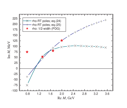
Figure 1: The complex $\mathcal{M}$-surface. Stars show location of the complex-mass resonances for leading $\rho$ Regge trajectory, where the imaginary-part component is the resonance half-width; data are from PDG tables [2]. Crosses show calculations with the use of eqs. (24) and (25).

More accurate calculations require accounting for the spin corrections, i.e., spin-spin and spin-orbit interactions. The spin-dependent corrections to the potential (2) have been calculated in [22] and can also be derived from lattice QCD, but we do not consider them here. In our case the spin corrections are accounted for effectively in parameters.

Note one important feature of the $\rho$-family resonance data. There is a dip ($\Gamma_{n}^{TOT}=107$ MeV) for the $a_{2}(1320)$ resonance (see Fig. 1). This dip is described by our model and has the following explanation. According to eq. (24) the imaginary-part mass ${\rm Im}\,\mathcal{M}_{n}$ can be positive and negative, i.e., poles can be embedded in the first and fourth-quarter of the complex $\mathcal{M}$-surface. Imaginary-part mass ${\rm Im}\,\mathcal{M}_{n}$ of the $\rho(770)$ resonance is negative. That means that the corresponding pole is embedded in the fourth quadrant of the complex $\mathcal{M}$-surface (i.e., Re$\,\mathcal{M}>0$, Im$\,\mathcal{M}<0$). But other poles of the $\rho$-family resonances are located above the real axis, i.e., in the bound state region.

5. Conclusion A thorough understanding of the physics summarized by the PDG is related to the concept of a resonance. Resonance in QM is closely connected with the concept of complex energy. In the version of QFT, the resonances are described by the complex-mass poles of the scattering matrix.

In contrast to the usual analysis dealing with the scattering problem, we have studied mesonic resonances to be the quasi-bound eigenstates of two interacting quarks using the Cornell potential. Using the complex-mass scheme we have analyzed the exact eigenvalues for the coulombic and linear terms of the potential, separately, and obtained the complex-mass formula for meson resonances. This approach has allowed us to simultaneously describe in the unified way the masses and total widths of resonances in a good agreement with data.

The complex-mass expression (4) may have relation to some non-hermitian Hamiltonian. In disagreement with a widely spread belief that the width of heavy hadronic resonances linearly depends on their mass, we have found this inconsistent with an existence of linear Regge trajectories. Widths obtained here are restricted or decreasing with the resonance mass.

Resonances represent a very economical way in theoretical description of hadronic reactions at high energies. Such a task is very important nowadays since a great significance of the width of heavy resonances. Our analysis may be important for further development of the string model of hadrons and for improvement of such transport codes as the hadron string dynamics by including the finite width of heavy resonances.

This work was done in the framework of investigations for the experiment ATLAS (LHC), code 02-0-1081-2009/2013, “Physical explorations at LHC” (JINR-ATLAS).

References

- [1]
- [2] J. Beringer et al. (Particle Data Group), Phys. Rev. D86, 010001 (2012).
- [3] N. Moiseyev, Phys. Rep. 302, 211 (1998).
- [4] J.R.Taylor, The Quantum Theory of Nonrelativistic Collisions, Dover Publications, 2006, 496 pages.
- [5] A.J.F. Siegert , Phys. Rev. 56, 750 (1939).
- [6] W. Heitler and N. Hu, Nature, 159, 776 (1947).
- [7] G. Rupp, S. Coito, E. Beveren, Acta Phys. Pol. B3 (2010), Proc. Supplement No 4.
- [8] T. Bauer, et al., Complex-mass scheme and resonances in EFT The 8th International workshop on the physics of excited nucleons: NSTAR 2011. AIP Conf. Proc., V. 1432, pp. 269-272 (2012) [arXiv:nucl-th/1107.5506v1]; A. Denner, S. Dittmaier, M. Roth and D. Wackeroth, Nucl. Phys. B560, 33 (1999).
- [9] L.D. Landau, E.M. Lifshitz, Quantum Mechanics, Pergamon, New York, 1965.
- [10] A. Bernicha, G.L. Castro and J. Pestieau, Nucl. Phys. A597, 623 (1996) [arXiv:hep-ph/9508388].
- [11] P.D. Hislop and C. Villegas-Blas [arXiv:math-ph/1104.4466v1]; M. Bander, C. Itzykson, Rev. Mod. Phys. 38(3), 330 (1966); R. Brummelhuis, A. Uribe, Commun. Math. Phys. 136, 567 (1991).
- [12] J. Nieves, E.R. Arriola, Phys. Lett. B679(5), 449 (2009).
- [13] J.D. Bjorken and E. Paschos, Phys. Rev. 185, 1975 (1969).
- [14] G.S. Bali, Phys. Rept. 343, 1-136 (2001); N. Brambilla, A. Pineda, J. Soto and A. Vairo, Rev. Mod. Phys. 77, 1423 (2005).
- [15] E. Eichten, S. Godfrey, H. Mahlke and J.L. Rosner, Rev. Mod. Phys. 80, 1161 (2008).
- [16] J. Sucher, Phys. Rev. D51, 5965 (1995); C. Semay and R. Ceuleneer, Phys. Rev. D48, 4361 (1993).
- [17] M.N. Sergeenko, Mod. Phys. Lett. A12, 2859 (1997) [arXiv:quant-ph/9911081].
- [18] M.N. Sergeenko, Phys. Rev. A53, 3798 (1996); [arXiv:quant-ph/9911075]; Mod. Phys. Lett. A15 (2000) 83; [arXiv:quant-ph/9912069]; Mod. Phys. Lett. A13 (1998) 33.
- [19] M.N. Sergeenko, Euro. Phys. J. C72(8), 2128 (2012) [arXiv:hep-ph/1206.7099].
- [20] M.N. Sergeenko, Europhys. Lett, 89, 11001 (2010); A Letter of Journal Exploring the Frontiers of Physics, EPL, Best of 2010, ISSN 0295-5075, P. 9 [arXiv:hep-ph/1107.1671]; Reports of Belarus Nat. Acad. Sci., 55(5), 40 (2011).
- [21] M.N. Sergeenko, Phys. At. Nucl. 56, 365 (1993).
- [22] M.N. Sergeenko, Z. Phys. C64, 315 (1994).
- [23] F. Cano, J.M. Laget, (DAPNIA, Saclay). Phys. Rev. D65, 074022 (2002).
- [24] M. Battaglieri et al. (CLAS Collaboration) Phys. Rev. Lett. 90, 022002 (2003).
- [25] J.M. Laget (DAPNIA, Saclay & Jefferson Lab), Phys. Rev. D70, 054023.12 (2004).
- [26] M. Battaglieri et al. (The CLAS Collaboration), Phys. Rev. Lett. 87, 172002 (2001).
- [27] L. Morand et al. (CLAS Collaboration) Eur. Phys. J. A24, 445 (2005); DAPNIA-05-54, JLAB-PHY-05-297, 2005.
- [28] P. Rossi for the collaboration JLAB-PHY-03-14, Physics of the CLAS collaboration: Some selected results, 2003, 11pp. Talk given at 41st International Winter Meeting on Nuclear Physics, Bormio, Italy, 26 Jan - 2 Feb 2003.
- [29] G.M. Huber, Charged Pion Electroproduction Ratios at High University of Regina Jefferson Lab PAC 30, Letter of Intent, Regina, SK S4S 0A2, Canada.
- [30] M.N. Sergeenko, Int. J. Mod. Phys. A18, 1 (2003) [arXiv:quant-ph/0010084].
- [31] P.D.B. Collins, An Introduction to Regge Theory and High-Energy Physics, Cambridge, England: Cambridge Univ. Press, 1977.
- [32] D. Morgan and M.R. Pennington, Phys. Rev. D48, 1185 (1993).
- [33] N. Fernández-García and O. Rosas-Ortiz, Ann. Phys 323, 1397-1414 (2008) [math-ph/arXiv:0810.5597]; [quant-ph/arXiv:0902.4061v1].
- [34] A textbook on Complex Analysis.