Latitudinal Dependence of Cosmic Rays Modulation at 1 AU and Interplanetary-Magnetic-Field Polar Correction

Abstract

The cosmic rays differential intensity inside the heliosphere, for energy below 30 GeV/nuc, depends on solar activity and interplanetary magnetic field polarity. This variation, termed solar modulation, is described using a 2-D (radius and colatitude) Monte Carlo approach for solving the Parker transport equation that includes diffusion, convection, magnetic drift and adiabatic energy loss. Since the whole transport is strongly related to the interplanetary magnetic field (IMF) structure, a better understanding of his description is needed in order to reproduce the cosmic rays intensity at the Earth, as well as outside the ecliptic plane. In this work an interplanetary magnetic field model including the standard description on ecliptic region and a polar correction is presented. This treatment of the IMF, implemented in the HelMod Monte Carlo code (version 2.0), was used to determine the effects on the differential intensity of Proton at 1 AU and allowed one to investigate how latitudinal gradients of proton intensities, observed in the inner heliosphere with the Ulysses spacecraft during 1995, can be affected by the modification of the IMF in the polar regions.

Accepted for publication on Advances in Astronomy

1 Introduction

The Solar Modulation, due to the solar activity, affects the Local Interstellar Spectrum (LIS) of Galactic Cosmic Rays (GCR) typically at energies lower than 30 GeV/nucl. This process, described by means of the Parker equation (e.g., see [1, 2] and Chapter 4 of [3]), is originated from the interaction of GCRs with the interplanetary magnetic field (IMF) and its irregularities. The IMF is the magnetic field that is carried outwards during the solar wind expansion. The interplanetary conditions vary as a function of the solar cycle which approximately lasts eleven years. In a solar cycle, when the maximum activity occurs, the IMF reverse his polarity. Thus, similar solar polarity conditions are found almost every 22 years [4]. In the HelMod Monte Carlo code version 1.5 (e.g., see Ref. [2]), the “classical” description of IMF, as proposed by Parker [5], was implemented together with the polar corrections of the solar magnetic field suggested subsequently in [6, 7]. This IMF was used inside the HelMod [2] code to investigate the solar modulation observed at Earth and to partially account for GCR latitudinal gradients, i.e., those observed with the Ulysses spacecraft [8, 9]. In order to fully account for both the latitudinal gradients and latitudinal position of the proton-intensity minimum observed during the Ulysses fast scan in 1995, the HelMod Code was updated to the version 2.0 to include a new treatment of the parallel and diffusion coefficients following that one described in Ref. [10]. In the present formulation, the parallel component of the diffusion tensor depends only on the radial distance from the Sun, while it is independent of solar latitude.

2 The Interplanetary Magnetic Field

Nowadays, we know that there is a Solar Wind plasma (SW) that permeates the interplanetary space and constitutes the interplanetary medium. In IMF models the magnetic-field lines are supposed to be embedded in the non-relativistic streaming particles of the SW, which carries the field with them into interplanetary space, producing the large scale structure of the IMF and the heliosphere. The “classical” description of the IMF was proposed originally by Parker (e.g., see [2, 5, 11, 12, 13, 14] and Chapter 4 of [3]). He assumed i) a constant solar rotation with angular velocity ($\omega$), ii) a simple spherically symmetric emission of the SW and iii) a constant (or approaching an almost constant) SW speed ($V_{\textrm{sw}}$) at larger radial distances ($r$), e.g., for $r>r_{b}\approx 10$R_⊙ (where R_⊙ is the Solar radius), since beyond $r_{b}$ the wind speed varies slowly with the distance. The “classical” IMF can be analytically expressed as [15]

$$\mathbf{B}_{Par}=\frac{A}{r^{2}}(\mathbf{e}_{r}-\Gamma\mathbf{e}_{\varphi})[1-2H(\theta-\theta^{\prime})],$$ (1)

where $A$ is a coefficient that determines the IMF polarity and allows $|\mathbf{B}_{Par}|$ to be equal to $B_{\oplus}$, i.e., the value of the IMF at Earth’s orbit as extracted from NASA/GSFC’s OMNI data set through OMNIWeb [16, 17]; $\mathbf{e}_{r}$ and $\mathbf{e}_{\varphi}$ are unit vector components in the radial and azimuthal directions, respectively; $\theta$ is the colatitude (polar angle); $\theta^{\prime}$ is the polar angle determining the position of the Heliospheric Current Sheet (HCS)[18]; $H$ is the Heaviside function: thus, $[1-2H(\theta-\theta^{\prime})]$ allows $\mathbf{B}_{Par}$ to change sign in the two regions above and below the HCS [18] of the heliosphere; finally,

$$\Gamma=\tan\Psi=\frac{\omega(r-r_{b})\sin\theta}{V_{\textrm{sw}}}$$ (2)

with $\Psi$ the spiral angle. In the present model $\omega$ is assumed to be independent of the heliographic latitude and equal to the sidereal rotation at the Sun’s equator. The magnitude of Parker field is thus:

$$B_{Par}=\frac{A}{r^{2}}\sqrt{1+\Gamma^{2}}.$$ (3)

	Period	Years
I)	$A<0$ Ascending	1964.79–1968.87, 1986.70–1989.54, 2008.95–2009.95
II)	$A<0$ Descending	1964.53–1964.79, 1979.95–1986.70, 2000.28–2008.95
III)	$A>0$ Ascending	1976.20–1979.95, 1996.37–2000.28
IV)	$A>0$ Descending	1968.87–1976.20, 1989.54–1996.37

Table 1: Definition of Ascending and Descending periods

Figure 1: (a) Maximum percentage difference between $B_{Pol}$ and $B_{Par}$ as a function of the solar distance inside the colatitude regions $20^{\circ}\leq\theta\leq 160^{\circ}$ ($\theta_{20^{\circ}}$), $25^{\circ}\leq\theta\leq 155^{\circ}$ ($\theta_{25^{\circ}}$) and $30^{\circ}\leq\theta\leq 150^{\circ}$ ($\theta_{30^{\circ}}$). (b) Maximum value allowed of $\delta_{m}$ as a function of colatitude: values in the “allowed” region guarantee that stream lines originated from the polar magnetic field do not cross the equatorial plane. Since Eq. (5) is symmetric with respect to the solar equatorial plane, values greater than 90^∘ of colatitude lead to same results of those presented.

In 1989 [6], Jokipii and Kóta have argued that the solar surface, where the feet of the field lines lie, is not a smooth surface, but a granular turbulent surface that keeps changing with time, especially in the polar regions. This turbulence may cause the footpoints of the polar field lines to wander randomly, creating transverse components in the field, thus causing temporal deviations from the smooth Parker geometry. The net effect of this is a highly irregular and compressed field line. In other words, the magnitude of the mean magnetic field at the poles is greater than in the case of the smooth magnetic field of a pure Parker spiral. Jokipii and Kóta [6] have therefore suggested that the Parker spiral field may be generalized by the introduction of a perturbation parameter [$\delta(\theta)$] which amplifies the field strength at large radial distances. With this modification the magnitude of IMF, Eq.(3), becomes [6]:

$$B_{Pol}=\frac{A}{r^{2}}\sqrt{1+\Gamma^{2}+\left(\frac{r}{r_{b}}\right)^{2}\delta(\theta)^{2}}.$$ (4)

The difference of the IMF obtained from Eq. (3) and Eq. (4) is less than $\sim$1% for colatitudes $20^{\circ}\leq\theta\leq 160^{\circ}$ (e.g, see Fig. 1a) and increases for colatitudes approaching the polar regions (e.g., see Figure 2 of [2]).

In the present treatment, the heliosphere is divided into polar regions and a equatorial region where different description of IMF are applied. In the equatorial region the Parker’s IMF, Eq. (3), is used, while in the polar regions we used a modified IMF that allows a magnitude as in Eq. (4):

$$\left\{\begin{array}[]{lll}\mathbf{B}_{Pol}&=\dfrac{A}{r^{2}}\left[\mathbf{e}_{r}+\dfrac{r}{r_{b}}\delta(\theta)\mathbf{e}_{\theta}-\dfrac{\omega(r-r_{b})\sin\theta}{V_{sw}}\mathbf{e}_{\varphi}\right]\left[1-2H\left(\theta-\theta^{\prime}\right)\right]&\textrm{Polar regions}\\ \\ \mathbf{B}_{Par}&=\dfrac{A}{r^{2}}\left[\mathbf{e}_{r}-\dfrac{\omega(r-r_{b})\sin\theta}{V_{sw}}\mathbf{e}_{\varphi}\right]\left[1-2H\left(\theta-\theta^{\prime}\right)\right]\!\!&\textrm{Equatorial region},\end{array}\right.$$ (5)

where equatorial regions are those with colatitude $X^{\circ}\leq\theta\leq(180^{\circ}-X^{\circ})$. The symbol $\theta_{X^{\circ}}$ indicates the corresponding polar regions.
In order to have a divergence-free magnetic-field we require that the perturbation factor [$\delta(\theta)$] has to be:

$$\delta(\theta)=\frac{\delta_{m}}{\left[1-2H\left(\theta-\theta^{\prime}\right)\right]\sin\theta},$$ (6)

where $\delta_{m}$ is the minimum perturbation factor of the field. The perturbation parameter is let to grow with decreasing of the colatitude. However, in their original work, Jokipii and Kóta [6] estimated the value of the parameter $\delta$ between $10^{-3}$ and $3\times 10^{-3}$.

Since the polar field is only a perturbation of the Parker field, it is a reasonable assumption that stream lines of the magnetic field do not cross the equatorial plane, thus, remaining completely contained in the solar hemisphere of injection. This allows one to estimate an upper limit on the possible values of $\delta_{m}$ [see Fig. 1(b)]. Currently, we use $\delta_{m}=1\times 10^{-5}$ by comparing simulations with observations at Earth orbit during Solar Cycle 23 (see Sect. 5).

HelMod Energy bin	KET channel
(0.35 – 0.98) GeV	(0.4 – 1.0) GeV
(0.76 – 2.09) GeV	(0.8 – 2.0) GeV
(2.09 – 200) GeV	$>2$ GeV

Table 2: Kinetic energy bins (in GeV) selected with HelMod Code and the corresponding proton energy channel for KET instruments on board the Ulysses spacecraft [8].

Energy range	$\theta_{\textrm{lat,min}}$ (in degrees)
	$\theta_{20^{\circ}}$	$\theta_{25^{\circ}}$	$\theta_{30^{\circ}}$
0.35 – 0.98 GeV	$-5^{+4}_{-5}$	$-8^{+4}_{-4}$	$-9^{+3}_{-3}$
0.76 – 2.09 GeV	$-5^{+6}_{-7}$	$-6^{+5}_{-6}$	$-10^{+4}_{-4}$
2.09 – 200 GeV	$-3^{+7}_{-7}$	$-7^{+7}_{-7}$	$-9^{+5}_{-6}$

Table 3: Latitudinal positions of minimum proton intensity ($\theta_{\textrm{lat,min}}$) (in degrees) as a function of the kinetic energy, using three values for the extension of the polar regions.

Energy range	$\Delta_{\textrm{N-S}}$ (%)
	$\theta_{20^{\circ}}$	$\theta_{25^{\circ}}$	$\theta_{30^{\circ}}$
0.35 – 0.98 GeV	$-8^{+6}_{-6}$	$-11^{+5}_{-4}$	$-13^{+4}_{-4}$
0.76 – 2.09 GeV	$-5^{+5}_{-6}$	$-6^{+5}_{-5}$	$-9^{+3}_{-3}$
2.09 – 200 GeV	$-1^{+3}_{-1}$	$-3^{+3}_{-3}$	$-4^{+2}_{-2}$

Table 4: Percentages of North-South asymmetry of proton intensities ($\Delta_{\textrm{N-S}}$) as a function of the kinetic energy, using three values for the extension of the polar regions.

Energy range	$\Delta_{\textrm{max}}$ (%)
	$\theta_{20^{\circ}}$	$\theta_{25^{\circ}}$	$\theta_{30^{\circ}}$
0.35 – 0.98 GeV	$-34^{+5}_{-5}$	$-35^{+4}_{-4}$	$-36^{+4}_{-3}$
0.76 – 2.09 GeV	$-22^{+6}_{-7}$	$-23^{+5}_{-4}$	$-25^{+3}_{-3}$
2.09 – 200 GeV	$-8^{+4}_{-3}$	$-9^{+3}_{-3}$	$-10^{+2}_{-2}$

Table 5: Differences in percentage between the maximum and minimum proton intensities ($\Delta_{\textrm{max}}$) as a function of the kinetic energy, using three values for the extension of the polar regions.

3 The Propagation Model

Parker in 1965 [1] (see also Ref. [2], Chapter 4 of [3] and references therein) treated the propagation of GCRs trough the interplanetary space. He accounted for the so-called adiabatic energy losses, outward convection due to the SW and drift effects. In the heliocentric system the Parker equation is then expressed (e.g. see [2, 19]):

$$\frac{\partial\mathrm{U}}{\partial t}=\frac{\partial}{\partial x_{i}}\left(K^{S}_{ij}\frac{\partial\mathrm{U}}{\partial x_{j}}\right)-\frac{\partial}{\partial x_{i}}[(V_{\mathrm{sw},i}+v_{d,i})\mathrm{U}]+\frac{1}{3}\frac{\partial V_{\mathrm{sw},i}}{\partial x_{i}}\frac{\partial}{\partial T}\left(\alpha_{\mathrm{rel}}T\mathrm{U}\right)$$ (7)

where $\mathrm{U}$ is the number density of particles per unit of particle kinetic energy $T$, at the time $t$. $V_{\mathrm{sw},i}$ is the solar wind velocity along the axis $x_{i}$ [20], $K^{S}_{ij}$ is the symmetric part of diffusion tensor [1], $v_{d}$ is the drift velocity that takes into account the drift of the particles due to the large scale structure of the magnetic field [21, 22, 23] and, finally,

$$\alpha_{\mathrm{rel}}=\frac{T+2m_{r}c^{2}}{T+m_{r}c^{2}},$$

where $m_{r}$ is the rest mass of the GCR particle. The last term of Eq. (7) accounts for adiabatic energy losses [1, 24]. The number density $\mathrm{U}$ is related to the differential intensity $J$ as ([2, 25], Chapter 4 of [3] and references therein):

$$J=\frac{vU}{4\pi},$$ (8)

where $v$ is the speed of the GCR particle.

Figure 2: Latitudinal relative intensity at $r=$ 1AU, obtained at different solar colatitudes for protons in the energy range defined in the Table 2 and using three definitions of polar regions: $\theta_{20^{\circ}}$, $\theta_{25^{\circ}}$ and $\theta_{30^{\circ}}$.

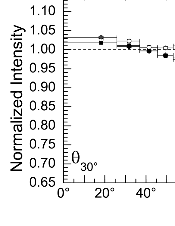
Figure 3: For the polar regions $\theta<30^{\circ}$ and $\theta>150^{\circ}$, latitudinal relative intensity at $r=$1 AU, accounting for GCR particles with $0^{\circ}<\theta<180^{\circ}$ ($\theta_{\textrm{R,0}}$), $1^{\circ}<\theta<179^{\circ}$ ($\theta_{\textrm{R,1}}$) and $2^{\circ}<\theta<178^{\circ}$ ($\theta_{\textrm{R,2}}$), respectively, are shown as a function of the proton kinetic energy and solar colatitude. Results with $10^{\circ}<\theta<170^{\circ}$ ($\theta_{\textrm{R,10}}$) are comparable with those obtained with $\theta_{\textrm{R,2}}$.

Equation (7) was solved using the HelMod code (see the discussion in Ref. [2]). This treatment (i) follows that introduced in Refs. [26, 27, 28, 29, 30, 10] and (ii) determines the differential intensity of GCRs using a set of approximated stochastic differential equations (SDEs) which provides a solution equivalent to that from Eq. (7). The equivalence between the Parker equation, that is a Fokker-Planck type equation, and the SDEs is demonstrated in [28, 31]. In the present work, we use a 2D (radius and colatitude) approximation for the particle transport. The model includes the effects of solar activity during the propagation from the effective boundary of the heliosphere down to Earth’s position.

The set of SDEs for the 2D approximation of Eq. (7) in heliocentric spherical coordinates is

$$\Delta r = \frac{1}{r^{2}}\frac{\partial}{\partial r}(r^{2}K^{S}_{rr})\Delta t-\frac{\partial}{\partial\mu(\theta)}\left[\frac{K^{S}_{r\mu}\sqrt{1-\mu^{2}(\theta)}}{r}\right]\Delta t$$ (9a)

$$+(V_{\rm{sw}}+v_{d,r})\Delta t+\left(2K^{S}_{rr}\right)^{1/2}\omega_{r}\sqrt{\Delta t},$$

$$\Delta\mu(\theta) = -\frac{1}{r^{2}}\frac{\partial}{\partial r}\left[rK^{S}_{\mu r}\sqrt{1-\mu^{2}(\theta)}\right]\Delta t+\frac{\partial}{\partial\mu(\theta)}\left[K^{S}_{\mu\mu}\frac{1-\mu^{2}(\theta)}{r^{2}}\right]\Delta t$$ (9b)

$$-\frac{1}{r}v_{d,\mu}\sqrt{1-\mu^{2}(\theta)}\Delta t-\frac{2K^{S}_{r\mu}}{r}\left[\frac{1-\mu^{2}(\theta)}{2K^{S}_{rr}}\right]^{1/2}\omega_{r}\sqrt{\Delta t}$$

$$+\frac{1}{r}\left\{[1-\mu^{2}(\theta)]\frac{K^{S}_{\mu\mu}K^{S}_{rr}-(K^{S}_{r\mu})^{2}}{0.5K^{S}_{rr}}\right\}^{1/2}\omega_{\mu}\sqrt{\Delta t},$$

$$\Delta T = -\frac{\alpha_{\rm rel}T}{3r^{2}}\frac{\partial V_{\rm sw}r^{2}}{\partial r}\Delta t,$$ (9c)

where $\mu(\theta)=\cos\theta$ and $\omega_{i}$ is a random number following a Gaussian distribution with a mean of zero and a standard deviation of one. The procedure for determining the SDEs can be found in [2].

In a coordinate system with one axis parallel to the average magnetic field and the other two perpendicular to this the symmetric part of the diffusion tensor $K^{S}_{ij}$ is (see e.g. [32]):

$$K^{S}_{ij}=\left[\begin{array}[]{ccc}K_{||}&0&0\\ 0&K_{\perp,r}&0\\ 0&0&K_{\perp,\theta}\end{array}\right]$$ (10)

with $K_{||}$ the diffusion coefficient describing the diffusion parallel to the average magnetic field, and $K_{\perp,r}$ and $K_{\perp,\theta}$ are the diffusion coefficients describing the diffusion perpendicular to the average magnetic field in the radial and polar directions, respectively. In this work $K_{||}$ is that one proposed by Strauss and collaborators in Ref. [10] (see also [33, 34, 35]):

$$K_{||}=\frac{\beta}{3}K_{0}\frac{P}{1\text{GV}}\left(1+\frac{r}{\text{1 AU}}\right),$$ (11)

where $K_{0}$ is the diffusion parameter - described in Section 2.1 of [2] -, which depends on solar activity and polarity, $\beta$ is the particle speed in unit of speed of light, $P=pc/|Z|e$ is the particle rigidity expressed in GV and, finally, $r$ is the heliocentric distance from the Sun in AU.

In the current treatment, $K_{||}$ has a radial dependence proportional to $r$, but no latitudinal dependence. Mc Donald and collaborators (see Ref. [36]) remarked that i) a spatial dependence of $K_{||}$ - like the one proposed here - can affect the latitudinal gradients at high latitude and ii) it is consistent with that originally suggested in Ref. [6]. Furthermore, the perpendicular diffusion coefficient is taken to be proportional to $K_{||}$ with a ratio $K_{\perp,i}/K_{||}=0.13$ for both $r$ and $\theta$ $i$-coordinates. The latter value is discussed in Sect. 5.

In addition, the practical relationship between $K_{0}$ and monthly Smoothed Sunspot Numbers (SSN) [37] values - discussed in Section 2.1 of [2] - is currently updated using the most recent data from Ref. [38]. As in Ref. [2], the $K_{0}$ data are subdivided into four sets, i.e., ascending and descending phases for both negative and positive solar magnetic-field polarities (Table 1). It has to be remarked that after each maximum the sign of the magnetic field (i.e., the $A$ parameter in Eq. (5)) is reversed. The updated practical relationships between $K_{0}$ in $\textrm{AU}^{2}\textrm{GV}^{-1}\,\textrm{s}^{-1}$ and SSN values for $1.4\leq$SSN$\leq 165$ for the four periods (from I up to IV, listed in Table 1) are

I) $$K_{0}=0.000297\!-\!2.9\!\cdot\!10^{-6}\text{SSN}\!+\!8.1\!\cdot\!10^{-9}\text{SSN}^{2}\!+\!1.46\!\cdot\!10^{-10}\text{SSN}^{3}\!-\!8.4\!\cdot\!10^{-13}\text{SSN}^{4}$$ (12a)

II) $$K_{0}=\left\{\begin{array}[]{ll}0.000304846-5.8\cdot 10^{-6}\text{SSN}&\text{if SSN}<=20\\ \frac{0.00195}{\text{SSN}}-2.3\cdot 10^{-10}\text{SSN}^{2}+9.1\cdot 10^{-5}&\text{if SSN}>20\end{array}\right.$$ (12d)

III) $$K_{0}=0.0002391-8.453\cdot 10^{-7}\text{SSN}$$ (12e)

IV) $$K_{0}=0.000247-1.175\cdot 10^{-6}\text{SSN}.$$ (12f)

The rms (root mean square) values of the percentage difference between values obtained with Eqs. (12) from those determined using the procedure discussed in Section 2.1 of [2] applied to the data from Ref. [38] were found to be 6.0%, 10.1%, 7.0% and 13.2% for the period I (ascending phase with $A<0$), II (descending phase with $A<0$), III (ascending phase with $A>0$) and IV (descending phase with $A>0$), respectively.

$\delta_{m}$ $(\times 10^{-5})$	$\rho_{k}$	“R” model	“L” model	No Drift
0.0	0.10	14.1	11.0	33.4
1.0	0.10	11.7	8.7	33.2
2.0	0.10	11.6	8.3	33.7
3.0	0.10	11.6	8.3	33.7
1.0	0.11	6.4	9.0	27.7
2.0	0.11	7.8	9.0	28.3
3.0	0.11	7.5	8.8	29.2
1.0	0.12	6.3	7.1	23.5
2.0	0.12	6.3	7.3	24.7
3.0	0.12	7.1	6.9	24.4
1.0	0.13	6.3	6.4	20.1
2.0	0.13	6.6	7.6	20.4
3.0	0.13	6.7	7.7	20.5
1.0	0.14	7.3	7.0	15.9
2.0	0.14	7.3	7.2	16.4
3.0	0.14	7.2	6.5	16.8

Table 6: Average values (last three columns) of $\eta_{\mathrm{rms}}$ (in percentage, %) as a function of $\delta_{m}$ $(\times 10^{-5})$ and $\rho_{k}$, for BESS–1997, AMS–1998, PAMELA-2006/08, obtained from Eq. (16) without enhancement of the diffusion tensor along the polar direction ($\rho_{E}=1$), using “R” and “L” models for the tilt angle and No Drift approximation. The differential intensities were calculated accounting for particles inside the heliospheric regions for which solar latitudes are lower than $|5.7^{\circ}|$.

Figure 4: Proton differential intensity determined with the HelMod code (continuous line) compared to the experimental data of BESS–1997; the dashed line is the LIS (see the text).

Figure 5: Proton differential intensity determined with the HelMod code (continuous line) compared to the experimental data of AMS-1998; the dashed line is the LIS (see the text).

Figure 6: Proton differential intensity determined with the HelMod code (continuous line) compared to the experimental data of PAMELA 2006/08; the dashed line is the LIS (see the text).

4 The Magnetic Field in the Polar Regions

Section 2 describes an IMF following the Parker Field with a small region around the poles in which such a field is modified. As already mentioned (see e.g.[6, 39, 40, 41, 42, 43]), the correction is needed to better reproduce the complexity of the magnetic field in those regions.

Moreover, Ulysses spacecraft (see e.g. [44, 45, 46]) explored the heliosphere outside the ecliptic plane up to $\pm 80^{\circ}$ of solar latitude at a solar distance from $\sim 1$ up to $\sim 5$ AU. Using these observations, the presence of latitudinal gradient in the proton intensity could be determined (e.g., see Figure 2 of Ref. [9] and Figure 5 of Ref. [8]). The data collected during the latitudinal fast scan (from September 1994 up to August 1995) show (a) a nearly symmetric latitudinal gradient with the minimum near ecliptic plane, (b) a southward shift of the minimum and (c) an intensity in the North polar region at $80^{\circ}$ exceeding the South polar intensity. In Ref. [9] a latitudinal gradient of $\sim 0.3\%$/degree  for proton with kinetic energy $>0.1$ GeV was estimated. While in Ref. [8] the analysis to higher energy was extended estimating a gradient of $\sim 0.22\%$/degree for proton with kinetic energy $>2$ GeV. The minimum in the charged particle intensity separating the two hemispheres of the heliosphere occurs $\sim 10^{\circ}$ South of the heliographic equator [9]. In addition, an independent analysis that takes into account the latitudinal motion of the Earth and IMP8 confirms a significant ($\sim 8^{\circ}\pm 2^{\circ}$) southward offset of the intensity minimum [9] for $T>100$ MeV proton. Furthermore in Ref. [8], a southward offset of about $\approx 7^{\circ}$ is evaluated; this offset of the intensity minimum results to be independent of the particle energy up to 2 GeV. Finally, in Ref. [9], the intensity in the North polar region at $80^{\circ}$ is observed to exceed the South polar intensity of $\sim 6\%$ for protons with $T>100$ MeV.

$\delta_{m}$ $(\times 10^{-5})$	$\rho_{k}$	“R” model	“L” model	No Drift
0.0	0.10	11.2	10.8	15.4
1.0	0.10	11.0	10.1	15.8
2.0	0.10	9.6	10.0	16.7
3.0	0.10	9.6	10.0	16.7
1.0	0.11	13.4	13.1	16.0
2.0	0.11	12.7	12.9	15.4
3.0	0.11	12.7	12.5	16.2
1.0	0.12	18.7	17.7	13.4
2.0	0.12	18.3	16.9	12.8
3.0	0.12	18.1	17.3	12.8
1.0	0.13	23.3	23.5	14.3
2.0	0.13	25.0	24.7	13.3
3.0	0.13	24.3	24.2	13.1
1.0	0.14	32.3	30.7	18.0
2.0	0.14	32.8	30.8	17.1
3.0	0.14	31.5	30.7	17.9

Table 7: Average values (last three columns) of $\eta_{\mathrm{rms}}$ (in percentage, %) as a function of $\delta_{m}$ $(\times 10^{-5})$ and $\rho_{k}$, for BESS–1999, BESS–2000, BESS–2002, obtained from Eq. (16) without enhancement of the diffusion tensor along the polar direction ($\rho_{E}=1$), using “R” and “L” models for the tilt angle and No Drift approximation. The differential intensities were calculated accounting for particles inside the heliospheric regions for which solar latitudes are lower than $|5.7^{\circ}|$.

Figure 7: Proton differential intensity determined with the HelMod code (continuous line) compared to the experimental data of BESS–1999; the dashed line is the LIS (see the text).

Figure 8: Proton differential intensity determined with the HelMod code (continuous line) compared to the experimental data of BESS–2000; the dashed line is the LIS (see the text).

Figure 9: Proton differential intensity determined with the HelMod code (continuous line) compared to the experimental data of BESS–2002; the dashed line is the LIS (see the text).

Using the present HelMod code (version 2.0), we could investigate i) the latitudinal gradient of GCR intensities resulting from solar modulation and ii) how the magnetic-field structure of the polar regions, as defined in Sect. 2, is able to influence the GCR spectra on the ecliptic plane. As previously defined, we denote with $\theta_{X^{\circ}}$ a polar region of amplitude $X^{\circ}$ from polar axis, i.e., $\theta<X^{\circ}$ and $\theta>180^{\circ}-X^{\circ}$. Three regions with $X^{\circ}=20^{\circ},\,25^{\circ}$ and 30^∘  were investigated. Outside any of these regions, the ratio between $B_{Pol}$ and $B_{Par}$ in Eq. (5) is less than $\sim$1% (see Fig. 1) and, thus, it ensures a smooth transition between polar and equatorial regions. For the purpose or this study we consider an energy binning closer to those presented in Ref. [8]. The KET instrument [47] collects proton data in three “channels” one with energies ranging from 0.038 GeV up to 2.0 GeV and two for particle with kinetic energy $T>0.1$ GeV and $T>2$ GeV, respectively. A successive re-analysis of the collected data allowed the authors to subdivide the 0.25–2 GeV “channel” in three “sub-channels” of intermediate energies. Since the Present Model is optimized - as discussed in Ref. [2] - for particles with rigidity greater than 1 GV (i.e., $\approx 0.444$ GeV), the present results are compared only with the corresponding “channel” or “sub-channels” suited for the corresponding energy range (see Table 2).

At 1 AU and as a function of the solar colatitude, the GCR intensities for protons are shown in Fig. 2. For a comparison with Ulysses observations, the modulated intensities of protons - resulting from HelMod code - were investigated from $80^{\circ}$ (North) and down to $-80^{\circ}$ (South). They were obtained using the HelMod code and selected using the energy bins reported in table 2. In Fig. 2, the latitudinal intensity distribution is normalized to the corresponding South Pole intensity. The quoted errors include statistical and systematic errors. The distributions were interpolated using a parabolic function expressed as:

$$I(\theta_{\textrm{lat}})=a+c(\theta_{\textrm{lat}}+d)^{2},$$ (13)

where $I(\theta_{\textrm{lat}})$ is the normalized intensity, $\theta_{\textrm{lat}}$ is the latitudinal angle and $a,b$ and $c$ are parameters determined from the fitting procedure. The so obtained fitted curves are shown as continuous lines in Fig. 2. Furthermore, the latitudinal positions of minimum intensity ($\theta_{\textrm{lat,min}}$), percentages of North-South asymmetry of intensities ($\Delta_{\textrm{N-S}}$) and differences in percentage between the maximum and minimum intensities ($\Delta_{\textrm{max}}$) were also determined from the fitting procedure and are listed in Table 3, Table 4 and Table 5, respectively. The quoted errors - following a procedure discussed in Ref. [2] - are derived varying the fitted parameters in order to obtain a value of the parameter $\eta_{\mathrm{rms,lat}}$ two times larger than the one resulting from the best fit ($I_{\mathrm{best}}$). $\eta_{\mathrm{rms,lat}}$ is defined as:

$$\eta_{\mathrm{rms.lat}}=\sqrt{\frac{\sum_{i}(\eta_{i,lat}/\sigma_{\eta,i,lat})^{2}}{\sum_{i}1/\sigma^{2}_{\eta,i,lat}}}$$ (14)

with

$$\eta_{i,lat}=\frac{I(\theta_{i})-I_{\mathrm{best}}(\theta_{i})}{I_{\mathrm{best}}(\theta_{i})},$$ (15)

where $\theta_{i}$ is the central value of the $i$th latitudinal bin of the differential intensity distribution and $\sigma_{\eta,i,lat}$ are the errors including the experimental and Monte Carlo uncertainties. For $\theta_{30^{\circ}}$, i.e., assuming a modified polar magnetic-field for $\theta<30^{\circ}$ and $\theta>150^{\circ}$, we found a general agreement with Ulysses observations. The position of $\theta_{\textrm{lat,min}}$ is compatible within the errors with one observed in Ref. [8], as well as the values of $\Delta_{\textrm{N-S}}$ and $\Delta_{\textrm{max}}$.

The HelMod code allows one to investigate the relevance of the treatment of the polar region magnetic-field with respect to the resulting modulation of GCR. Thus, the latitudinal normalized intensities were obtained excluding a few (small) regions nearby the poles. This was determined from reducing the latitudinal spatial phase-space admissible for pseudo-particles (see Ref. [2]) - i.e., the latitudinal extension of GCR particles taken into account - to $1^{\circ}<\theta<179^{\circ}$ ($\theta_{\textrm{R,1}}$), $2^{\circ}<\theta<178^{\circ}$ ($\theta_{\textrm{R,2}}$) and $10^{\circ}<\theta<170^{\circ}$ ($\theta_{\textrm{R,10}}$). The so obtained latitudinal gradients are compared with the full latitudinal extension, $\theta_{\textrm{R,0}}$ ($0^{\circ}<\theta<180^{\circ}$), in Fig. 3. By an inspection of Fig. 3, one may lead to the conclusion that the GCR diffusion nearby the polar axis has a large impact on the latitudinal gradients in the inner heliosphere. As a consequence, the IMF description in the polar regions is relevant in order to reproduce the observed modulated GCR spectra.

5 Comparison with Observations During Solar Cycle 23

The agreement of HelMod simulated spectra with observations during solar cycle 23 is investigated via quantitative comparisons using Eqs. (16) and (17). However, since the structure of the heliosphere is different in high and low solar activity the two periods are separately analyzed.

The HelMod Code [2] (version 2.0) allowed us to investigate how the modulated (simulated) differential intensities are affected by the (1) particle drift effect, (2) polar enhancement of the diffusion tensor along the polar direction ($K_{\perp,\theta}$, e.g., see Ref. [48]), and, finally, (3) values of the tilt angle ($\alpha_{t}$) calculated following the approach of the “R” and “L” models [49]. This analysis also allow us to estimate the values of IMF parameters that better describe the modulation along the entire solar cycle. The effects related to particle drift were investigated via the suppression of the drift velocity (No Drift approximation), this accounts for the hypothesis that magnetic drift convection is almost completely suppressed during solar maxima. The differential intensities were calculated for $K_{\perp,\mu}=\rho_{E}K_{\perp,r}$ with values of $\rho_{E}$ of 1, 8 and 10, i.e., no enhancement, that suggested in Ref. [50] and that suggested in Ref. [48, 2] (and reference there in), respectively. Furthermore, the modulated proton spectra were derived from a LIS whose normalization constant depends on the experimental set of data and were already discussed in Ref. [2]). In addition, the differential intensities were calculated accounting for particles inside heliospheric regions where solar latitudes are lower than $|5.7^{\circ}|$.

During the period of high solar activity for the solar cycle 23, the BESS collaboration took data in the years 1999, 2000, and 2002 (see sets of data in Ref. [51]). For period not dominated by high solar activity in solar cycle 23, BESS, AMS and PAMELA collaborations took data, i.e., BESS–1997 [51], AMS–1998 [52], and PAMELA–2006/08 [53].

Following the procedure described in Ref. [2], the observation data were compared with those obtained from HelMod code using the error-weighted root mean square ($\eta_{\mathrm{rms}}$) of the relative difference ($\eta$) between experimental data ($f_{\mathrm{exp}}$) and those resulting from simulated differential intensities ($f_{\mathrm{sim}}$). For each set of experimental data and with the approximations and/or models described above, we determined the quantity

$$\eta_{\mathrm{rms}}=\sqrt{\frac{\sum_{i}(\eta_{i}/\sigma_{\eta,i})^{2}}{\sum_{i}1/\sigma^{2}_{\eta,i}}}$$ (16)

with

$$\eta_{i}=\frac{f_{\mathrm{sim}}(T_{i})-f_{\mathrm{exp}}(T_{i})}{f_{\mathrm{ref}}(T_{i})},$$ (17)

where $T_{i}$ is the average energy of the $i$th energy bin of the differential intensity distribution and $\sigma_{\eta,i}$ are the errors including the experimental and Monte Carlo uncertainties; the latter account for the Poisson error of each energy bin. The simulated differential intensities are interpolated with a cubic spline function. The modulation results are studied varying the parameters $\delta_{m}$ - from 0, i.e., the non-modified Parker IMF, up to $3\times 10^{-5}$, see Fig. 1(b) -, $K_{\perp,r}/K_{||}=\rho_{k}$ (from 0.10 up to 0.14) and $K_{\perp,\theta}/K_{\perp,r}=\rho_{E}$ (from 1 up to 10) seeking a set of parameters set that minimize $\eta_{\mathrm{rms}}$. In Table 6, the average values of $\eta_{\mathrm{rms}}$ (in percentage, %) for low solar activity periods are listed. They were obtained in the energy range  from 444 MeV up to 30 GeV using the “L” and “R” models for the tilt angle $\alpha_{t}$ and for the No Drift approximation and without any enhancement of the diffusion tensor along the polar direction ($K_{\perp,\mu}$). The results derived with the enhancement of the diffusion tensor along the polar direction indicate that for $\rho_{E}=$ 8 and 10 one obtains a value of $\eta_{\mathrm{rms}}$ that is from 1.5 up to 3 times larger with respect the case without enhancement. From inspection of Table 6, one can remark that the drift mechanism leads to a better agreement with experimental data. Furthermore the, “R” and “L” models for tilt angles are comparable within the precision of the method (discussed in Ref. [2]). The minimum difference with respect to the experimental data occurs when $\rho_{k}=0.11-0.13$ and $\delta_{m}=1.0\times 10^{-5}$ for both “R” and “L” models, with the “L” model slightly preferred to “R”.

In Figs. 4–6, the differential intensities determined with the HelMod code are shown and compared to the experimental data of BESS–1997, AMS–1998, and PAMELA–2006/08, respectively; in these figures, the dashed lines are the LIS as discussed in Ref. [2]. These modulated intensities are the ones calculated for a heliospheric region where solar latitudes are lower than $|5.7^{\circ}|$, using $\rho_{k}=0.13$, $\delta_{m}=1.0\times 10^{-5}$ and $\rho_{E}=1$ with the “L” model. Finally, one can remark that the present code, combining diffusion and drift mechanisms, is also suited to describe the modulation effect in periods when the solar activity is no longer at the maximum.

In Table 7 we present the averages $\eta_{\mathrm{rms}}$ (in percentage, %) during the periods dominated by high solar activity. The simulated differential intensities were obtained for a heliospheric region where solar latitudes are lower than $|5.7^{\circ}|$ without any enhancement of the diffusion tensor along the polar direction ($K_{\perp,\mu}$). The simulations with $\rho_{E}=$ 8 and 10 lead to $\eta_{\mathrm{rms}}$ comparable with those presented in Table 7. However, using $\rho_{E}=1$ provides a better agreement to experimental data at lower energy. From inspection of Table 7, one can note that “R” and “L” models for tilt angles yield comparable results within the precision of the method. Furthermore the minimum difference with the experimental data occurs when $\rho_{k}=0.10$ and $\delta_{m}=(2.0$–$3.0)\times 10^{-5}$ with the“L” model slightly preferred to “R”. The HelMod parameter configuration, which minimizes the difference to the experimental data, are reported in Table 8: one may remark that the No Drift approximation is (almost) comparable to a drift treatment for both BESS–2000 and BESS–2002 with data collected during and after the maximum of the solar activity. Apparently, the drift treatment is needed in order to describe BESS–1999 with data taken during a period approaching the solar maximum.

Observations	“R” model	“L” model	No Drift
BESS–1999	9.3	10.6	25.7
BESS–2000	12.5	12.6	16.7
BESS–2002	6.9	6.7	7.7

Table 8: Average $\eta_{\mathrm{rms}}$ (in percentage, %), for BESS–1999, BESS–2000, BESS–2002, obtained from Eq. (16) without enhancement of the diffusion tensor along the polar direction ($\rho_{E}=1$), $\delta_{m}=2.0\times 10^{-5}$, $\rho_{k}=0.10$ and using “R” and “L” models for the tilt angle and No Drift approximation. The differential intensities were calculated accounting for particles inside the heliospheric regions for which solar latitudes are lower than $|5.7^{\circ}|$.

In Figs. (7)–(9), the differential intensities determined with the HelMod code are shown and compared with the experimental data of BESS–1999, BESS–2000, and BESS–2002, respectively; in these figures, the dashed lines are the LIS as discussed in Ref. [2]. These modulated intensities are the ones calculated for a heliospheric region where solar latitudes are lower than $|5.7^{\circ}|$, using $K_{\perp,\mu}=K_{\perp,r}$ independently of the latitude and including particle drift effects with the values of the tilt angle from the “L” model. Finally, it is concluded that the present code combining diffusion and drift mechanisms is suited to describe the modulation effect in periods with high solar activity [2, 50, 54].

6 Conclusion

In this work an IMF, which combines the Parker Field and its polar modification, is presented. In the polar regions, the Parker IMF was modified with an additional latitudinal components according to those proposed by Jokipii and Kóta in Ref. [6]. We found the maximum perturbed value with this component yielding, as a physical result, streaming lines completely confined in the solar hemisphere of injection.

The proposed IMF is, then, used within the HelMod Monte Carlo code to determine the effects on the differential intensity of protons at 1 AU as a function of the extension of polar region, in which the modified magnetic-field is employed. We found that a polar region contained within 30^∘ of colatitude is that one ensuring a very smooth transition to the equatorial region and allows to reproduce qualitatively and quantitatively the latitudinal profile of the GCR intensity, and the latitudinal dip shift with respect to the ecliptic plane. Finally we determined how the polar region diffusion is mostly responsible of the proton intensity latitudinal gradient observed in the inner heliosphere with the Ulysses spacecraft during 1995.

References

References

- [1] E. N. Parker. The passage of energetic charged particles through interplanetary space. Plan. Space Sci., 13:9, 1965.
- [2] P. Bobik, G. Boella, M. J. Boschini, C. Consolandi, S. Della Torre, M. Gervasi, D. Grandi, K. Kudela, S. Pensotti, P. G. Rancoita, and M. Tacconi. Systematic Investigation of Solar Modulation of Galactic Protons for Solar Cycle 23 Using a Monte Carlo Approach with Particle Drift Effects and Latitudinal Dependence. Astrophys. J., 745:132, February 2012.
- [3] C. Leroy and P.-G. Rancoita. Principles of Radiation Interaction in Matter and Detection, 3rd Edition. World Scientific Publishing Co, 2011.
- [4] R. D. Strauss, M. S. Potgieter, and S. E. S. Ferreira. Modeling ground and space based cosmic ray observations. Adv. Space Res., 49:392–407, January 2012.
- [5] E. N. Parker. Dynamics of the interplanetary gas and magnetic fields. Astrophys. J., 128:664, 11 1958.
- [6] J. R. Jokipii and J. Kota. The polar heliospheric magnetic field. Geophys. Res. Lett., 16:1–4, Jan 1989.
- [7] U.W. Langner. Effect of termination shock acceleraion on cosmic ray in the helisphere. PhD thesis, Potchestroom University, Potchestroom, 2004.
- [8] B. Heber, W. Droege, P. Ferrando, L. J. Haasbroek, H. Kunow, R. Mueller-Mellin, C. Paizis, M. S. Potgieter, A. Raviart, and G. Wibberenz. Spatial variation of 40MeV/n nuclei fluxes observed during the ULYSSES rapid latitude scan. Astron. Astrophys., 316:538–546, December 1996.
- [9] J. A. Simpson. Ulysses cosmic-ray investigations extending from the south to the north polar regions of the Sun and heliosphere. Nuovo Cimento C, 19:935–943, December 1996.
- [10] R. D. Strauss, M. S. Potgieter, I. Büsching, and A. Kopp. Modeling the Modulation of Galactic and Jovian Electrons by Stochastic Processes. Astrophys. J., 735:83, July 2011.
- [11] E. N. Parker. Newtonian Development of the Dynamical Properties of Ionized Gases of Low Density. Phys. Rev., 107:924–933, August 1957.
- [12] E. N. Parker. The Hydrodynamic Theory of Solar Corpuscular Radiation and Stellar Winds. Astrophys. J., 132:821, November 1960.
- [13] E. N. Parker. Sudden Expansion of the Corona Following a Large Solar Flare and the Attendant Magnetic Field and Cosmic-Ray Effects. Astrophys. J., 133:1014, May 1961.
- [14] E. N. Parker. Interplanetary dynamical processes. New York, Interscience Publishers, 1963., 1963.
- [15] M. Hattingh and R. A. Burger. A new simulated wavy neutral sheet drift model. Adv. Space Res., 16(9):213–216, 1995.
- [16] J. H. King and N. E. Papitashvili. Solar wind spatial scales in and comparisons of hourly Wind and ACE plasma and magnetic field data. J. Geophys. Res.-Space, 110(A9):A02104, February 2005.
- [17] NASA-OMNIweb. online database http://omniweb.gsfc.nasa.gov/form/dx1.html, 2012.
- [18] J. R. Jokipii and B. Thomas. Effects of drift on the transport of cosmic rays. IV - Modulation by a wavy interplanetary current sheet. Astrophys. J., 243:1115–1122, February 1981.
- [19] J. R. Jokipii, E. H. Levy, and W. B. Hubbard. Effect of particle drift on cosmic-ray transport. i. general properties, application to solar modulation. Astrophys. J. Lett., 213:L85–L88, April 1977.
- [20] E. Marsch, W. I. Axford, and J. F. McKenzie. Solar wind. In B. N. Dwivedi, editor, Dynamic Sun, pages 374–402, 2003.
- [21] J. R. Jokipii and E. H. Levy. Effects of particle drifts on the solar modulation of galactic cosmic rays. Astrophys. J. Lett., 213:L85–L88, April 1977.
- [22] M. S. Potgieter and H. Moraal. A drift model for the modulation of galactic cosmic rays. Astrophys. J., 294(part 1):425–440, 1985.
- [23] R. A. Burger and M. Hattingh. Steady-State Drift-Dominated Modulation Models for Galactic Cosmic Rays. Astroph. and Sp. Sc., 230:375–382, August 1995.
- [24] J. R. Jokipii and E. N. Parker. On the Convection, Diffusion, and Adiabatic Deceleration of Cosmic Rays in the Solar Wind. Astroph. J., 160:735, May 1970.
- [25] L. J. Gleeson and W. I. Axford. Solar Modulation of Galactic Cosmic Rays. Astrophys. J., 154:1011, December 1968.
- [26] Y. Yamada, S. Yanagita, and T. Yoshida. A stochastic view of the solar modulation phenomena of cosmic rays. Geophys. Res. Lett., 25:2353–2356, July 1998.
- [27] M. Gervasi, P. G. Rancoita, I. G. Usoskin, and G. A. Kovaltsov. Monte-Carlo approach to Galactic Cosmic Ray propagation in the Heliosphere. Nucl. Phys. B - Proc. Sup., 78:26–31, August 1999.
- [28] M. Zhang. A Markov Stochastic Process Theory of Cosmic-Ray Modulation. Astrophys. J., 513:409–420, March 1999.
- [29] K. Alanko-Huotari, I. G. Usoskin, K. Mursula, and G. A. Kovaltsov. Stochastic simulation of cosmic ray modulation including a wavy heliospheric current sheet. J. Geophys. Res., 112:A08101, 2007.
- [30] C. Pei, J. W. Bieber, R. A. Burger, and J. Clem. A general time-dependent stochastic method for solving Parker’s transport equation in spherical coordinates. J. Geophys. Res.-Space, 115(A12107), December 2010.
- [31] C.W. Gardiner. Handbook of stochastic methods: for physics, chemistry and natural sciences. Springer Edition, 1985.
- [32] J. R. Jokipii. Propagation of cosmic rays in the solar wind. Rev. Geoph. Space Phys., 9:27–87, 1971.
- [33] I. D. Palmer. Transport coefficients of low-energy cosmic rays in interplanetary space. Rev. Geophys. Space Ge., 20:335–351, May 1982.
- [34] M. S. Potgieter and S. E. S. Ferreira. Effects of the solar wind termination shock on the modulation of Jovian and galactic electrons in the heliosphere. J. Geophys. Res.-Space, 107:1089, July 2002.
- [35] W. Dröge. Probing heliospheric diffusion coefficients with solar energetic particles. Adv. Space Res., 35:532–542, 2005.
- [36] F. B. McDonald, P. Ferrando, B. Heber, H. Kunow, R. McGuire, R. Müller-Mellin, C. Paizis, A. Raviart, and G. Wibberenz. A comparative study of cosmic ray radial and latitudinal gradients in the inner and outer heliosphere. J. Geophys. Res., 102:4643–4652, March 1997.
- [37] SIDC-team. The International Sunspot Number. Monthly Report on the International Sunspot Number, online catalogue, 1964-2010.
- [38] I. G. Usoskin, G. A. Bazilevskaya, and G. A. Kovaltsov. Solar modulation parameter for cosmic rays since 1936 reconstructed from ground-based neutron monitors and ionization chambers. J. Geophys. Res.-Space, 116:A02104, February 2011.
- [39] A. Balogh, E. J. Smith, B. T. Tsurutani, D. J. Southwood, R. J. Forsyth, and T. S. Horbury. The Heliospheric Magnetic Field Over the South Polar Region of the Sun. Science, 268:1007–1010, May 1995.
- [40] H. Moraal. Proton Modulation Near Solar Minimim Periods in Consecutive Solar Cycles. In International Cosmic Ray Conference, volume 6, page 140, 1990.
- [41] C. W. Smith and J. W. Bieber. Solar cycle variation of the interplanetary magnetic field spiral. Astroph. J., 370:435–441, March 1991.
- [42] L. A. Fisk. Motion of the footpoints of heliospheric magnetic field lines at the Sun: Implications for recurrent energetic particle events at high heliographic latitudes. J. Geophys. Res., 101:15547–15554, July 1996.
- [43] M. Hitge and R. A. Burger. Cosmic ray modulation with a Fisk-type heliospheric magnetic field and a latitude-dependent solar wind speed. Adv. Space Res., 45:18–27, January 2010.
- [44] T. R. Sanderson, R. G. Marsden, K.-P. Wenzel, A. Balogh, R. J. Forsyth, and B. E. Goldstein. High-Latitude Observations of Energetic Ions During the First ULYSSES Polar Pass. Space Sci. Rev., 72:291–296, April 1995.
- [45] R. G. Marsden. The 3-D Heliosphere at Solar Maximum. The Publications of the Astronomical Society of the Pacific, 113:129–130, January 2001.
- [46] A. Balogh, R. G. Marsden, and E. J. Smith. The heliosphere near solar minimum. The Ulysses perspective. Springer-Praxis Books in Astrophysics and Astronomy, 2001.
- [47] B. Heber, M. S. Potgieter, and P. Ferrando. Solar modulation of galactic cosmic rays: the 3D heliosphere. Adv. Space Res., 19:795–804, May 1997.
- [48] M. S. Potgieter. Heliospheric modulation of cosmic ray protons: Role of enhanced perpendicular diffusion during periods of minimum solar modulation. J. Geophys. Res., 105:18295–18304, 2000.
- [49] J. T. Hoeksema. The Large-Scale Structure of the Heliospheric Current Sheet During the ULYSSES Epoch. Space Sci. Rev., 72:137–148, April 1995.
- [50] S. E. S. Ferreira and M. S. Potgieter. Long-Term Cosmic-Ray Modulation in the Heliosphere. Astrophys. J., 603:744–752, March 2004.
- [51] Y. Shikaze, S. Orito, T. Mitsui, and BESS Collaboration. Measurements of 0.2 20 GeV/n cosmic-ray proton and helium spectra from 1997 through 2002 with the BESS spectrometer. Astrop. Phys., 28:154–167, 2007.
- [52] M. Aguilar, J. Alcaraz, J. Allaby, and AMS Collaboration. The Alpha Magnetic Spectrometer (AMS) on the International Space Station: Part I - results from the test flight on the space shuttle. Phys. Rep., 366:331–405, 2002.
- [53] O. Adriani, G. C. Barbarino, G. A. Bazilevskaya, and PAMELA Collaboration. PAMELA Measurements of Cosmic-Ray Proton and Helium Spectra. Science, 332:69, 2011.
- [54] D. C. Ndiitwani, S. E. S. Ferreira, M. S. Potgieter, and B. Heber. Modelling cosmic ray intensities along the Ulysses trajectory. Annales Geophysicae, 23:1061–1070, March 2005.