Entropic commensurate-incommensurate transition
Abstract
The equilibrium properties of a minimal tiling model are investigated. The model has extensive ground state entropy, with each ground state having a quasiperiodic sequence of rows. It is found that the transition from the ground state to the high temperature disordered phase proceeds through a sequence of periodic arrangements of rows, in analogy with the commensurate-incommensurate transition. We show that the effective free energy of the model resembles the Frenkel-Kontorova Hamiltonian, but with temperature playing the role of the strength of the substrate potential, and with the competing lengths not explicitly present in the basic interactions.
pacs:
PACS numbers: 64.60.De , 61.44.Fw, 61.44.BrTilings provide a simple means to model systems with both simple and complex ground states. As statistical mechanical models, they include such systems as the Ising and Potts models, as well as other models with discrete spin variablesfn1 . The class of tilings, however, is much largertilings_and_patterns , and includes the various non-periodic Wang tilingsfn2 , the quasiperiodic Penrose tilings, the asymptotically isotropic Pinwheel tilingpinwheel , and the recently discovered generalizations of the Rudin-Shapiro sequence, which are neither periodic nor quasiperiodicWolff .
The statistical mechanical behavior of tiling models is rich, and, as yet, largely uncharted. Apart from results which may be transcribed from discrete spin models, only a very small number of systems have been studied. First, a model based on the Amman set of 16 Wang tiles with quasiperiodic ground states was studied by several authors leuzzi_thermodynamics_2000 ; rotman_finite-temperature_2011 ; koch_modelling_2010 . It appears that this model undergoes a continuous phase transition from a disordered state to a quasiperiodic phase, and its non-equilibrium behavior was studied in the context of spin-glasses. A variation of the model allowing more complicated interactions and vacancies shows a first order transitionaristoff_first_2011 . Hierarchical tilingsmiekisz_microscopic_1990 have also been studied, and a very recent modelbyington_hierarchical_2012 possesses limit-periodic ground states which undergo a series of phase transitions where motifs of ever larger scales order as the temperature is lowered. Finally, we note some recent studies sasa_pure_2012 ; sasa_statistical_2012 on models with large number of degenerate disordered ground states aimed at studying glasses.
In this paper we study the equilibrium behavior of a model based on the 13-tile Kari-Culik (KC) set culik_ii_aperiodic_1996 ; kari_small_1996 of Wang tiles, both numerically and analytically. The KC set is the smallest known aperiodic set - it is the smallest set of tiles which can tile the plane, but not periodically. Allowed juxtapositions of tiles are enforced by matching rules, and these in turn induce a Hamiltonian: Every matching rule violation is penalized by a positive energy, while allowed matchings have zero energy. In what follows, we shall denote the energy cost of mismatching adjacent vertical or horizontal edges by or , respectively.
We shall argue that the equilibrium behavior of this system is analogous to the Frenkel-Kontorova (FK) modelchaikin_principles_2000 of the commensurate-incommensurate (CI) transition. The FK model describes a chain of masses which are connected by springs and subjected to a periodic substrate potential. It exhibits rich behavior due to competition between these two interactions, each of which favors ordering with a different wavelength. However, in marked contrast with the FK model, where the favored length scales are present in the Hamiltonian, in the KC model they emerge spontaneously, from only nearest-neighbor interactions. Moreover, the role of substrate potential strength in the FK model is played by the temperature in the KC model. In this sense, the KC system exhibits an entropic CI transition.
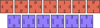
As indicated in Figure 1, the 13 KC tiles may be divided into two groups, which we will call types A and B. The markings on the edges of the tiles indicate the matching rules - abutting edges of adjacent tiles have the same markings in a perfect tiling. It is readily seen that in an undefected tiling, a given row can consist of A or B type tiles only, with no mixing, and thus, we may characterize a row as being A-type or B-type.
The KC tiling differs from other tilings studied in that it is not generated by recursive substitution (inflation)tilings_and_patterns , and by the fact that it has a ground state degeneracy with extensive entropy. This should be contrasted with tilings created from a simple inflation rule where the degeneracy scales as a power of the system sizekoch_modelling_2010 . All the ground states, however, are characterized by a quasiperiodic arrangement of A-type and B-type rows. The finite temperature behavior of this model is striking - as the temperature is increased from zero, the rows, still identifiable as A or B type, order periodically with decreasing period. At high enough temperatures, the rows lose their A or B identity, and the system becomes disordered.
The proof that there exists a zero-energy ground state is equivalent to showing that a perfect tiling exists. To do thisEigen , we note that there are two numbers which characterize the row in a perfect tiling - the “frequency” and the number which are related through the mapping
| (1) |
where
| (2) |
Note that we shall take n to increase in the -y direction.
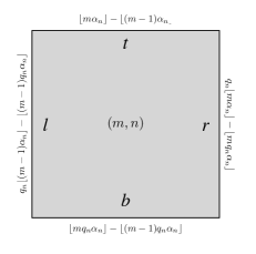
The reason for dividing the tile set into the A and B groups becomes apparent if we denote the markings of the top, bottom, right, and left edges of a tile by {t,b,r,l}, as shown in Figure 2. When needed, we shall indicate the position of the tile as a subscript; thus refers to the marking of the top edge of the tile centered at (m,n), etc. It is easily verified by inspecting Figure 1 that the markings on each tile satisfy the relation
| (3) |
with a tile of type or having or , respectively. The mapping has no periodic points, since for any positive integers and ; this implies that the resultant tilings are not periodic. The are distributed densely, but not uniformly, in the range .
To show that a perfect tiling exists, we must solve Equations 3 for all m,n with derived from Equations 1 and 2 whilst demanding that and . It is easily verified that the markings
| (4) | |||||
constitutes a solution, where is the greatest integer less than or equal to (see Figure 2); this is one example of a perfect tiling.
To facilitate later discussion, we shall employ a useful mapping. Let us define the variable , where . Decomposing into its integer and fractional parts gives
| (5) |
where , the fractional part of , is defined through its relation to by
| (6) |
This maps onto , and allows us to obtainfuturepub an explicit formula for :
Sequences of this type are called Sturmian sequences, and are well known in the context of automatic sequencesallouche_automatic_2003 . Here is irrational, and this gives a quasiperiodic sequence of the two “letters” and , with the consequence that in the ground state the rows appear in a quasiperiodic sequence.

As noted above, this ground state is only one of many, and in fact, there is an extensive ground state entropyfuturepub . This may be inferred from Figure 3, where two patches with the same markings on their exterior are presented (there exist larger patches with the same property as well). This means that starting from some given ground state, we may obtain another by randomly exchanging the patches shown in Figure 3 (and any other pair of patches with the same exterior markings), provided, as we have verifiedfuturepub , that they appear with a finite density in the ground state. This implies that almost all of the ground states are disordered in the sense that their patch entropykurchan_levine scales as the patch size for large enough patches. This notwithstanding, in all the ground states, the rows are arranged in a quasiperiodic sequence of A-type and B-type, and it is also true that is unchanged for each rowfuturepub , which is relevant to what follows.
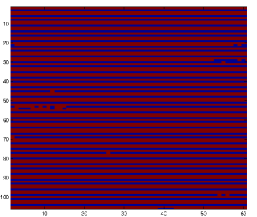
Numerical studies of this model show that as the temperature is raised from 0, it goes through a series of phase transitions, where the A-B sequence of rows is periodic, and where the period decreases with increasing temperature. In analogy to the CI transition, we shall refer to these periodic phases as commensurate phases. In Figure 4, we show a portion of a time averaged configuration from a system (with ) at (in units of ), which was obtained by parallel tempering, where the color coding is as in Figure 1. The A-B sequence is periodic with period 8, with 3 B rows per period. Characteristic defects are also present. At high enough temperature, of course, the rows lose their A or B character, and the system goes to a disordered phase.
The different phase transitions are best traced by the winding number . Since at low T the rows are essentially pure type A or B, essentially counts the fraction of type B rows in the system. For an ensemble of systems at any given temperature, may take a variety of values, where the distribution has a well-defined maximum value, , which is typically close but not identical to the average 111The distinction between and will vanish in the thermodynamic limit.. For large systems, both and will equal at and approach as . The first order nature of the transitions between the different commensurate phases can be verified by looking at the distribution of near the transitions, which exhibits two well separated peaks, with one overtaking the other as the transition temperature is crossed futurepub . This suggests that is a reliable indicator of these transitions.
In Figure 5 we show curves of and the specific heat vs. T, for a system. At low temperature, the system is in its ground state, and (to within ). As temperature is increased, undergoes three jump discontinuities before becoming fully continuous as the rows are no longer homogeneous. While the step-wise behavior of is a clear indication of the existence of the commensurate phases and the first order nature of the transitions between them, its value at the plateaus does not give the exact periodicities due to limited resolution and the existence of defects, and these then must be inferred by looking at the configurations themselves, as in Figure 4. The first order transitions are accompanied by small bumps in the specific heat at the same temperatures. In Figure 5, we identify phases with periods of and rows with the lower and middle plateaus, respectively. In our examinations of systems of sizes up to , we have identified phases with and , depending on system size and values of the coupling constants. At these temperatures, we have verified numerically that the rows substantially maintain their pure A or B character. The broad peak in the specific heat at attends the loss of purity in the rows.
These results may be understood by an effective coarse-grained description of this system, appropriate for low temperatures, when the system may be considered as composed of A and B type rows222Although this is easiest to justify when , our numerical study indicates that it has a large range of validity even when .. This description resembles the Frenkel-Kontorova modelchaikin_principles_2000 , and exhibits a competition between length scales. To see this, note that for the perfect tiling, the value of the frequency for the row may be calculated from the tile markings: . From this, using Equations 5 and 6, we can compute . Now although defects enter the rows at finite , we may still define two frequencies, using the markings of the top and bottom of a row. The “top frequency” is defined as while the “bottom frequency” is given by . For a perfect tiling, , and therefore, from Equation 1, , but this will typically not be the case for defected tilings. This notwithstanding, the at finite may be inferred from using Equation 6 in the same manner as for the perfect tiling. These will be the variables used in our effective description.
To construct an effective free energy for this model we assume that the dominant contributions come from the entropy of the rows, and the energy due to mismatches between the rows, each of which is characterized by its frequencies and . We argue that the energy cost associated with an imperfect interface between rows and goes as , where L is the length of the row. Clearly, this term is zero in the ground state, and numerical simulations bear out this functional form for low temperaturesfuturepub . At this level of coarse graining, a row is characterized by its frequency (or equivalently ), and its entropy should be a function of this frequency which is extensive in L, so that we shall write the entropy of the row as .
Taken together, we get that the free energy is given by . It is convenient to express this in terms of the variables discussed above. The free energy is then of the form
| (7) |
where is a function that favors , which holds identically in the ground state. The entropy depends only on the fractional part , and thus it is a periodic function with period one. It is the competition between these two length scales which gives the novel behavior observed. Although it is tempting to expand to first order as , we note that such an expression fails when both and are larger than , since this would imply two adjacent B rows, which carries a disproportionately large energy cost.
The equilibrium configuration of the can be obtained by minimizing . As in the FK model, the first term favors an incommensurate phase with a winding number while the entropy favors a commensurate configuration. The temperature plays the role of the strength of the periodic potential, so that commensurate phases are expected at high temperature while incommensurate phases are expected at low temperatures. The commensurate phases that are expected are those with a winding number close to such as , etc. We have observed some of these phases in our numerical study, as seen in Figure 5, where their presence is indicated by the plateau values of . At still higher temperatures the segregation into type A and B rows breaks down, resulting in a disordered phase. It is interesting to speculate about the low T behavior of this system. It might be that only at an incommensurate phase appears, but it could be that such a phase, possibly with power-law correlations, is stable at finite T. These issues will be addressed in future work.
We would like to thank P. Chaikin, J. Kurchan, T. Lubensky, F. Sausset, and G. Wolff for fruitful discussions. D.L. gratefully acknowledges support from Israel Science Foundation grant 1574/08 and US-Israel Binational Science Foundation grant 2008483.
References
- (1) As distinct, for example, from the Heisenberg or x-y models, which employ continuous spins.
- (2) Wang tilings employ square tiles, and as such may be used to model systems on a square lattice.
- (3) J. Allouche and J. Shallit. Automatic Sequences: Theory, Applications, Generalizations. Cambridge University Press, 2003.
- (4) D. Aristoff and C. Radin. First order phase transition in a model of quasicrystals. J. Phys. A, 44(25):255001, 2011.
- (5) T. Byington and J. Socolar. Hierarchical freezing in a lattice model. Phys. Rev. Lett., 108:045701, 2012.
- (6) P. M. Chaikin and T. C. Lubensky. Principles of Condensed Matter Physics. Cambridge University Press, reprint edition, 2000.
- (7) K. Culik II. An aperiodic set of 13 wang tiles. Discrete Math., 160:245–251, 1996.
- (8) J. Eigen, S. Navarro and V. Prasad. An aperiodic tiling using a dynamical system and beatty sequences. Recent Progress in Dynamics, 54:207, 2007.
- (9) B. Grünbaum and G. Shephard. Tilings and Patterns. W.H. Freeman and Company, reprint edition, 1987.
- (10) J. Kari. A small aperiodic set of wang tiles. Discrete Math., 160:259–264, 1996.
- (11) H. Koch and C. Radin. Modelling quasicrystals at positive temperature. J. Stat. Phys., 138(1):465–475, 2010.
- (12) J. Kurchan and D. Levine. Order in glassy systems. J. Phys. A., 44(3):035001, 2011.
- (13) L. Leuzzi and G. Parisi. Thermodynamics of a tiling model. J. Phys. A, 33(23):4215–4225, 2000.
- (14) J. Miekisz. A microscopic model with quasicrystalline properties. J. Stat. Phys., 58(5):1137–1149, 1990.
- (15) N. Nikola, D. Hexner, and D. Levine. To be published.
- (16) C. Radin. The pinwheel tilings of the plane. The Ann. Math., 139(3):pp. 661–702, 1994.
- (17) Z. Rotman and E. Eisenberg. Finite-temperature liquid-quasicrystal transition in a lattice model. Phys. Rev. E, 83(1):011123, 2011.
- (18) S.-i. Sasa. Pure glass in finite dimensions. arXiv:1203.2406, 2012.
- (19) S.-i. Sasa. Statistical mechanics of glass transition in lattice molecule models. J. Phys. A, 45(3):035002, 2012.
- (20) G. Wolff and D. Levine. to be published.