A Customized 3D GPU Poisson Solver for Free Boundary Conditions

Abstract

A 3-dimensional GPU Poisson solver is developed for all possible combinations of free and periodic boundary conditions (BCs) along the three directions. It is benchmarked for various grid sizes and different BCs and a significant performance gain is observed for problems including one or more free BCs. The GPU Poisson solver is also benchmarked against two different CPU implementations of the same method and a significant amount of acceleration of the computation is observed with the GPU version.

1 Introduction

In the context of electronic structure calculations of molecules, wires, surfaces and solids, it is necessary to solve Poisson’s equation with various boundary conditions (BCs), namely free BCs, wire BCs (periodic along one axis, free along two axes), surface BCs (periodic along two axes, free along one axis) and fully periodic boundary conditions.

A common method for solving the Poisson’s equation

$$\nabla^{2}V=\rho$$ (1)

exploits the Fast Fourier Transform (FFT) algorithm in order to transform the input density $\rho$ into the Fourier space. The desired electrostatic potential $V$ can then easily be found in Fourier space and it is converted back to the real space by an inverse FFT. This FFT based solution is preferred for large data sets because of its $O(N\mbox{Log}N)$ scaling due to the FFTs, $N$ being the number of grid points for the discrete representation of the density $\rho$ and the solution $V$. This method is also suitable for GPU computation since FFTs are efficiently implemented for GPUs by various vendors and groups [1, 2, 3, 4]. Currently the NVIDIA CUFFT library supports 1D, 2D and 3D FFTs both for real and complex input data in single and double precision.

In current GPU architectures, the data array has to be transferred to the device memory prior to the computation and the result has to be transferred back to the system memory to be used in the succeeding CPU parts of the code. These data transfer times are comparable to the GPU computation times for the Poisson solver case, reducing the possible gains of GPUs for such calculations. The situation is less problematic for the case of free BCs since the transferred data size for such problems is half of the FFT size for each dimension. For a 3D input data, which is usually encountered in physical problems, the transferred data size is reduced to one eighth of the total FFT size, making the problem suitable for GPU computation. As the number of axis with free boundary conditions decreases when going from fully free boundary conditions to fully periodic boundary conditions, the data size increases to a quarter, a half and finally the full FFT data set size and the transfer times dominate more and more. Additionally, 3D FFT computation time for free BC problems can be reduced by using customized algorithms since initially only one eighth of the 3D FFT size is non-zero, remaining being zero padded [5].

Some GPU based Poisson solvers can be found in the literature. In the work of Deck and Singh [6] the CUFFT library is used in the FFT based solution of the 2D Poisson’s equation for periodic BCs. Rossinelli et al. [7] use the same technique for a 2D free BCs problem. However, they do not use a specialized algorithm to avoid calculations over zero padded regions but they apply multidimensional FFTs on the full zero padded domain. Beside these FFT based works, there are some iterative GPU Poisson solvers [8, 9] which do not exploit the $O(N\mbox{Log}N)$ scaling of FFTs.

In this work, we describe a GPU Poisson solver which uses customized 3D FFTs to increase the performance for free BCs. This customized GPU Poisson solver is benchmarked for various grid sizes for fully free, wire and surface BCs to see the possible gain in the presence of free BCs. It is also benchmarked against a CPU implementation of the same method which uses the FFTW library [10] for 1D batched FFTs. The developed GPU Poisson was implemented in the BigDFT wavelet based electronic structure package [11, 12, 13] and benchmarked against the current CPU Poisson solver of BigDFT [14] for fully free BCs.

2 Poisson’s Equation

In the discretized integral form, the Poisson’s equation (Eq. 1) for a periodic input density becomes a convolution of the form:

$$V({\bf r})=\sum_{r^{\prime}}K_{p}({\bf r}-{\bf r^{\prime}})\rho({\bf r^{\prime}})~{},$$ (2)

where $K_{p}({\bf r}-{\bf r^{\prime}})$ is the Green’s function associated with the periodic BCs. This equation can be solved easily in Fourier space just with a multiplication operation:

$$V^{F}({\bf k})=K_{p}^{F}({\bf k})\rho^{F}({\bf k})~{},$$ (3)

where the superscript $F$ denotes the Fourier transform of the corresponding quantity which can be calculated by the FFT algorithm. Once the potential is calculated in Fourier space with the above formula, it can be converted back to the real space with an inverse FFT operation. The advantage of this strategy is that the convolution in Eq. 2 is calculated in $O(N\mbox{Log}N)$ operations instead of the $O(N^{2})$ operations of the direct calculation, where $N=N_{x}N_{y}N_{z}$ is the total number of grid points in the 3-dimensional input density.

Poisson’s equation with free BCs can be treated similarly by using the free boundary Green’s function $K_{f}$ instead of $K_{p}$ in Eq. 3. Since the use of a FFT implies periodicity, free boundary conditions can only be achieved by zero padding to the input density, doubling its size in each dimension [7, 15, 16]. In this way the wrap arounds in FFTs can be avoided at the cost of enlarging the problem size. For a mixed BCs problem, the zero paddings should be applied for all the dimensions having free BCs. Examples of these mixed BCs problems are surfaces with one free dimension and wires with two free dimensions for which the associated Green’s functions have to be used in the calculation [17].

3 Customized GPU Poisson Solver

In our GPU Poisson solver, we implemented the method used in the Poisson solver of the BigDFT electronic structure package [14]. For free BC dimensions, the input density is zero padded doubling the data size for that dimension. Direct application of 3D FFT libraries for such a zero padded input data is not efficient since these algorithms work on the whole range regardless of the data being zero or not. In our developments, a customized 3D FFT is used for this problem which avoids the calculation of 1D FFTs over the zero padded parts of the input density.

Basically, a 3D FFT can be calculated in three steps each having 1D FFTs of all the rows in a separate dimension. In our customized 3D FFT, zero padded parts of the data are identified for each dimension and the unnecessary calculations over these parts are avoided. To understand the algorithm let us denote the data size in three dimensions as $N_{x}$,$N_{y}$ and $N_{z}$ and the BCs as $B_{x}$, $B_{y}$ and $B_{z}$ having values $1$ for periodic and $2$ for free BCs. Then the FFT size for each dimension is given as $S_{j}=N_{j}\times B_{j}$. In the first step, 1D FFTs of length $S_{x}$ should be calculated for $N_{y}\times N_{z}$ rows instead of the full range of $S_{y}\times S_{z}$ rows. For the second dimension, 1D FFTs of length $S_{y}$ should be calculated for $S_{x}\times N_{z}$ rows since non-zero elements emerge in the zero padded parts of the $x$-dimension after the first step. In the third step the whole size of $S_{x}\times S_{y}$ rows should be processed for $S_{z}$ length 1D FFTs. Therefore, for a fully free boundary problem, the total number of 1D FFT operations is reduced to $7/12$ (approximately $58\%$) of the direct calculation of the whole zero padded range with a 3D FFT library such as CUFFT3D. Inverse of the zero padding operations are carried out for the inverse 3D FFT after the multiplication in Eq. 3, as compactifications of the data by taking out unnecessary parts. Therefore, the same amount of reduction in the computation time is also valid for the inverse 3D FFT. For the heterogeneous BCs cases (surface and wire BCs), the reduction amount of 1D FFT operations is influenced by the choice of the axes along which free dimensions are applied (one axis for surface BCs and two axes for wire BCs). If the free dimension(s) is/are chosen as the last dimension(s) of the forward transform then the zero paddings can be postponed and the performance of the method increases. In the inverse transform, free BC dimension(s) are processed first since the order of axes reverses for this case. For the wire BCs, if the periodic dimension is chosen as the first dimension of the forward 3D FFT then the reduction of 1D FFT operations is the same as the fully free BCs discussed above. The total performance for wire BCs is slightly better than the fully free BCs of same zero padded size since for the wire case there is no need for the initial zero padding operation before the FFTs in the first dimension (also the final compactification in the inverse FFT). For the surface BCs, by choosing the free BC dimension as the last dimension of the forward 3D FFT, the number of the 1D FFT operations reduces to $2/3$ (approximately $66\%$) of the fully periodic case.

In the calculation of a 3D FFT, a transposition operation usually follows each of the three steps described above in order to conserve the desired access pattern for optimal performance [18]. Such transpositions are also used in our customized 3D GPU FFT in order to preserve the coalesced access pattern to the global memory for the computations in three separate dimensions. If the zero paddings for the free BCs treatment are applied in the beginning of the calculation for all free boundary dimensions then the zero parts of the data should also be processed during the transpositions. In order to avoid these unnecessary operations, zero padding operations are applied for dimensions having free BCs just before the FFTs in that dimensions by a spread operation which doubles the data length for each row and sets the first half to zero. (In the inverse FFT, compactification operations are carried out after the FFTs in each dimension having free BCs, as throwing out the second half of each row.) In this strategy the transpositions are applied with reduced data sets and additionally the zero padding spread GPU kernel (also the compactification kernel in inverse FFT) can be merged with the preceding transpose GPU kernel (except for the first dimension which does not have the transposition) to reduce the number of read/write operations to the GPU global memory. As an example, for fully free BCs the first transposition operation between the first two dimensions of the forward transform is carried out with a data size which is a quarter of the total zero padded FFT size since the second and the third dimensions are not zero padded at that moment. The second transposition between the second and the third dimensions is carried out with the half of the total zero padded FFT size since the last dimension is not zero padded yet. The final transposition after the third dimension should be operated on the full size but this transposition can be eliminated completely with a transposition of the associated kernel of the convolution in Eq. 3 which is carried out only once in the multiple application of the Poisson solver which is usually the case in realistic applications.

Since the input density for the Poisson solver is always a real valued quantity it would be advantageous to use real to complex FFTs for the first dimension of the forward 3D FFT. Because of the property $F_{N-n}=F_{n}^{*}$ of a real to complex FFT it is enough to keep first $S_{x}/2+1$ terms of the result after the 1D FFTs in the first dimension and the succeeding 1D FFTs in the remaining dimensions are carried out over this reduced data set of size $(S_{x}/2+1)\times S_{y}\times S_{z}$. It is not necessary to unfold the result at the end of the FFT for the Poisson solver case since an inverse FFT follows the forward FFT yielding a real potential at the end. The complex to real 1D FFTs for the last dimension of this inverse transform has the same symmetry mentioned above.

Separate steps of the customized GPU algorithm are given below where bold text is used to indicate the GPU kernels. Processed data size is indicated for each 1D FFT step. The transpose or transpose+spread (compactification+transpose for inverse FFT) kernels process same size of data as the preceding 1D FFTs:

• if (B_x is free) spread_X

• 1DFFT_X ($N_{y}\times N_{z}$ rows, length $S_{x}$) (R2C)

• if (B_y is free) transpose+spread_Y

  else transpose

• 1DFFT_Y ($(S_{x}/2+1)\times N_{z}$ rows, length $S_{y}$)

• if (B_z is free) transpose+spread_Z

  else transpose

• 1DFFT_Z ($(S_{x}/2+1)\times S_{y}$ rows, length $S_{z}$)

• convolution kernel multiplication

• inverve_1DFFT_Z ($(S_{x}/2+1)\times S_{y}$ rows, length $S_{z}$)

• if (B_z is free) compactification_Z+transpose

  else transpose

• inverse_1DFFT_Y ($(S_{x}/2+1)\times N_{z}$ rows, length $S_{y}$)

• if (B_y is free) compactification_Y+transpose

  else transpose

• inverse_1DFFT_X ($N_{y}\times N_{z}$ rows, length $S_{x}$) (C2R)

• if (B_x is free) compactification_X

In the implementation of the method we used the NVIDIA CUFFT1D library for evaluating batched 1D FFTs and the CUDA language for transpositions and spread (compactification) operations. The method was tested with NVIDIA CUDA Toolkit version 4.1 on a NVIDIA Tesla series M2090 GPU using double precision. An OpenCL implementation of the method using custom 1D FFT GPU kernels is also in progress.

4 Results

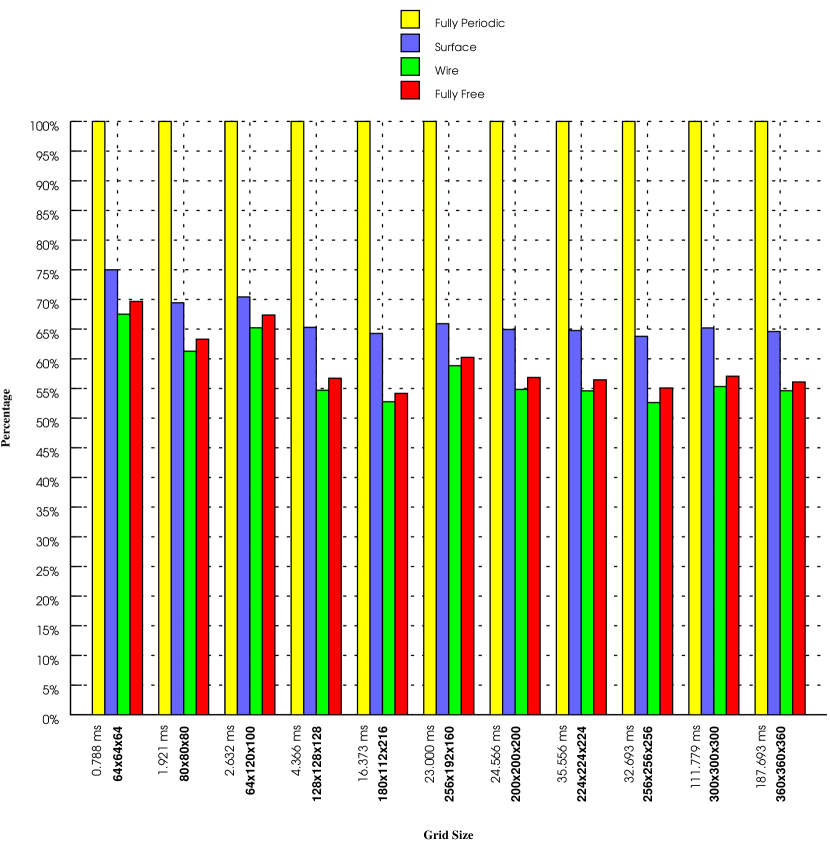
Figure 1: Comparison of the GPU computation times for different BCs. Fully free, wire and surface BCs computation times are shown as percentages of fully periodic BCs computation times which are given under corresponding column bars in milliseconds. The grid sizes given in the figure are FFT sizes ($S_{x}\times S_{y}\times S_{z}$) after the zero paddings in necessary dimensions.

Benchmark calculations for fully periodic, surface, wire and fully free BCs are carried out by varying the grid size. Computation times for the fully periodic case not including the data transfers and computation times of the cases having one or more free boundary dimensions relative to the fully periodic case are given in Figure 1 for different grid sizes. In the figure, grid sizes are always given as the zero padded FFT sizes ($S_{x}\times S_{y}\times S_{z}$) instead of the input density sizes in order to keep FFT sizes constant for different BCs, yielding a better comparison of the results. The computation time percentages for the free BCs case and the wire BCs case are close to the calculated percentage of $58\%$ for the amount of 1D FFTs except for the small grid dimensions. Small deviations from this value are due to the spread, transposition and convolution kernel multiplication operations which become more important for small grid dimensions. For the surface BCs, again the computation time percentages are close to the calculated percentage of $66\%$ for the amount of 1D FFTs except for the small grid dimensions and the variations can be explained with the same reasoning as the free and wire BCs cases.

Performance of the customized GPU Poisson solver in the presence of free dimensions is compared also with a CPU implementation of the same method where FFTW library is used for batched 1D FFTs and CUDA kernels for spread and transposition operations are replaced with corresponding CPU functions in C programming language. Intel compiler version 11.1 is used in the compilation with default optimization level (-O2) and sse2 instructions are enabled in the compilation of the FFTW library. An Intel I7 930 2.8 GHz Quad Core processor is used in these CPU calculations and the comparison is made against single core and also against 4 cores using OpenMP parallelization. GPU computation times with and without data transfer times are given for fully free, surface and wire BCs in Figure 2 relative to single core CPU computation times and in Figure 3 relative to 4 cores CPU computation times. Grid sizes are given as the zero padded FFT sizes ($S_{x}\times S_{y}\times S_{z}$) also for these comparisons. For the single core case, computation time ratios between the CPU implementation and the GPU implementation vary in between $7.798$ and $24.389$ depending on the grid size and BCs. For the 4 cores CPU case the range of this ratio is between $2.769$ and $11.090$. When the transfer times of sending the input density to the device memory and getting the resulted potential from the device memory are also included in the comparison, the computation time ratios of the CPU case to the GPU case vary in between $2.879$ and $15.602$ for single core case and this ratio is between $1.154$ and $6.815$ for 4 cores CPU case.

In order to test the developed GPU Poisson solver in a real application, we implemented it in the BigDFT electronic structure package and compared its performance with the CPU Poisson solver of the BigDFT for fully free BCs which is faster than the CPU implementation using FFTW for fully free BCs since it takes advantage of merging transpose and kernel multiplication operations with customized 1D FFTs. These comparison results are given in Figure 4 and Figure 5 for single core CPU and 4 cores CPU respectively. Including data transfer times, for the single core case computation time ratios between the CPU implementation and the GPU implementation vary in between $4.967$ and $14.922$ depending on the grid size. For the 4 cores CPU case the range of this ratio is between $1.610$ and $4.189$.

5 Conclusions

We have developed a customized GPU Poisson solver which is generally applicable to homogeneous and mixed BCs. Benchmark calculations show significant reduction of computation times compared to the fully periodic BCs case for the cases having one or more free BCs. The largest reduction of computation times are observed in the case of wire BCs where the periodic dimension is chosen as the first dimension of the forward 3D FFT. The reductions of computation times compared to the fully periodic case are in consistence with the reduction of total number of 1D FFT operations and these reductions would not be observed in the direct application of a 3D FFT library for these cases with one or more free BC dimensions. Instead, in such a direct application, the computation times would slightly increase compared to the fully periodic case because of the additional zero padding spread operations and corresponding compactifications. However, the developers of various 3D FFT libraries may benefit from the techniques described in this work to increase the performance of their libraries for such zero padded input data.

Comparison with CPU computations shows that the customized GPU Poisson solver provides up to $\sim$24.4 times faster computations compared to single core CPU computation when data transfer times are not considered. With the advent of new hardware which merges CPU and GPU on the same chip and with new technologies like NVIDIA GPUDirect [19] which allows calling MPI subroutines between GPU memories, transfers to and from the GPU will be required less frequently and it will be possible to run a large fraction of sophisticated software packages on the GPU. Also, when multiple solution of the Poisson’s equation from different input densities are required (as it is the case, for example, in Quantum Chemistry or electronic structure calculations), the transfer time for a given density can be overlapped by the calculation of the previous one [12, 13]. For these reasons we give also the speedups without the transfer times. Even when the transfer times are included, the customized GPU Poisson solver provides up to $\sim$15.6 times faster computations compared to single core CPU. This means that the developed GPU Poisson solver can be used in real applications including free BCs to accelerate the Poisson solver part of the code. Figures 2 and 3 show that the performance gain from GPU computation reduces for small sizes and it is maximal for large power of two sizes. Increase of the data transfer to computation time ratios with increasing number of periodic dimensions is also evident in these Figures. Therefore, when data transfer times are also considered, the amount of acceleration due to GPU usage increases as the number of free dimensions increases.

The new developments are implemented in the BigDFT Electronic Structure Package version 1.7 and the Poisson solver part of the code is accelerated as shown in Figure 4 and Figure 5 for fully free BCs calculations. Up to $\sim$14.9 times acceleration compared to single core CPU is observed in these tests including data transfer times. For surface and wire BCs, the comparison was not carried out since BigDFT code does not consider the optimal order of periodic and free dimensions for these mixed BCs cases at the moment. The source code of the BigDFT package can be accessed from the BigDFT project web page [20] under GPL License agreement.

The convolution operation which is the main part of the Poisson solver discussed in this work is not only required in the context of solving Poisson’s equation, but also in many other contexts. In plane wave density functional programs, the application of the local potential onto the wave function is for instance a convolution of the same type as the convolution in the solution of Poisson’s equation with free BCs. Such programs have also been ported to GPU’s [21] but the possible speedup that could be obtained in this context by a customized FFT has not been exploited so far.

Acknowledgements: We thank Peter Messmer from NVIDIA Corp. for his suggestions and valuable discussions about the subject.

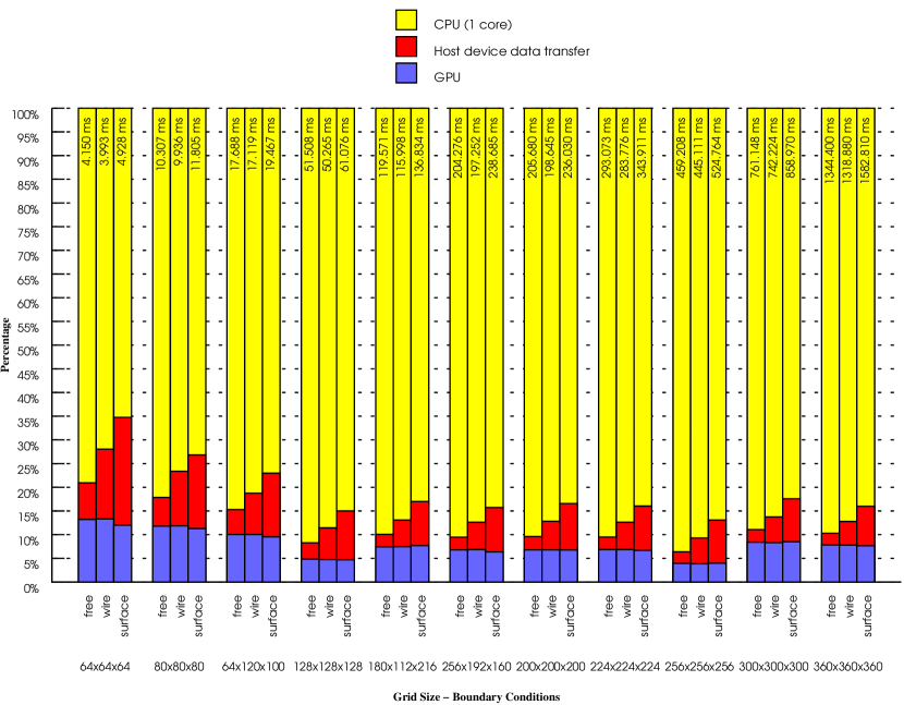
Figure 2: Comparison of the GPU computation times with FFTW implementation single core CPU computation times. GPU and GPU + data transfer times are shown as percentages of single core CPU computation times for different grid sizes for fully free, wire and surface BCs. Single core CPU computation times are given on each column bar in milliseconds. The grid sizes given in the figure are FFT sizes ($S_{x}\times S_{y}\times S_{z}$) after the zero paddings in necessary dimensions.

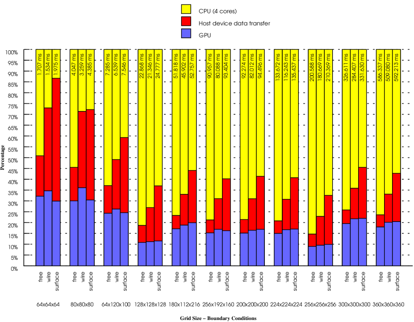
Figure 3: Comparison of the GPU computation times with FFTW implementation 4 cores CPU computation times. GPU and GPU + data transfer times are shown as percentages of 4 cores CPU computation times for different gird sizes for fully free, wire and surface BCs. 4 cores CPU computation times are given on each column bar in milliseconds. The grid sizes given in the figure are FFT sizes ($S_{x}\times S_{y}\times S_{z}$) after the zero paddings in necessary dimensions.

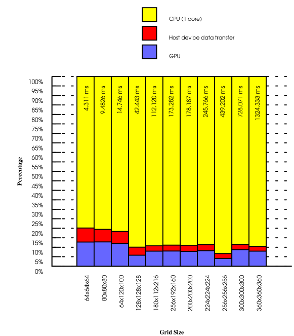
Figure 4: Comparison of the GPU computation times with BigDFT Poisson solver single core CPU computation times for fully free BCs. GPU and GPU + data transfer times are shown as percentages of single core CPU computation times for different grid sizes. Single core CPU computation times are given on each column bar in milliseconds. The grid sizes given in the figure are FFT sizes ($S_{x}\times S_{y}\times S_{z}$) after the zero paddings in all dimensions.

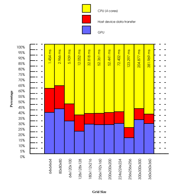
Figure 5: Comparison of the GPU computation times with BigDFT Poisson solver 4 cores CPU computation times for fully free BCs. GPU and GPU + data transfer times are shown as percentages of 4 core CPU computation times for different grid sizes. 4 cores CPU computation times are given on each column bar in milliseconds. The grid sizes given in the figure are FFT sizes ($S_{x}\times S_{y}\times S_{z}$) after the zero paddings in all dimensions.

References

- Nukada et al. [2008] A. Nukada, Y. Ogata, T. Endo, S. Matsuoka, Bandwidth intensive 3-D FFT kernel for GPUs using CUDA, in: SC ’08:Proceedings of the 2008 ACM/IEEE Conference on Supercomputing, IEEE Press, Piscataway,NJ,USA, 2008, pp. 1–11.
- Govindaraju et al. [2008] N. K. Govindaraju, B. Lloyd, Y. Dotsenko, B. Smith, J. Manferdelli, High Performance Discrete Fourier Transforms on Graphics Processors, in: SC ’08:Proceedings of the 2008 ACM/IEEE Conference on Supercomputing, IEEE Press, Piscataway,NJ,USA, 2008.
- Volkov and Kazian [2008] V. Volkov, B. Kazian, Fitting FFT onto the G80 architecture, http://www.cs.berkeley.edu/~kubitron/courses/cs258-S08/projects/reports/project6_report.pdf, 2008.
- cuf [2012] NVIDIA Corp. CUDA CuFFT Library, 2012.
- Goedecker [1991] S. Goedecker, Efficient pseudopotentials and algorithms for electronic structure calculations based on density functional theory, Ph.D. thesis, Ecole Polytechnique Fédérale de Laussane, 1991.
- Decyk and Singh [2011] V. Decyk, T. Singh, Adaptable Particle-in-Cell algorithms for graphical processing units, Comput. Phys. Commun. 182 (2011) 641.
- Rossinelli et al. [2010] D. Rossinelli, M. Bergdorf, G. Cottet, P. Koumoutsakos, GPU accelerated simulations of bluff body flows using vortex particle methods, J. Comput. Phys. 229 (2010) 3316.
- A. Kosior [2012] H. K. A. Kosior, Parallel computations on gpu in 3D using the vortex particle method, Comput. Fluids (2012).
- Knittel [2010] G. Knittel, A CG-based Poisson Solver on a GPU-Cluster, High Performance Computing (HiPC), 2010 International Conference on (2010) 1.
- Frigo and Johnson [2005] M. Frigo, S. Johnson, The design and implementation of FFTW3, Proc. IEEE 93 (2005) 216.
- Genovese et al. [2008] L. Genovese, A. Neelov, S. Goedecker, T. Deutsch, S. Ghasemi, A. Willand, D. Caliste, O. Zilberberg, M. Rayson, A. Bergman, R. Schneider, Daubechies wavelets as a basis set for density functional pseudopotential calculations, J. Chem. Phys. 129 (2008) 014109.
- Genovese et al. [2009] L. Genovese, M. Ospici, T. Deutsch, J. Mehaut, A. Neelov, S. Goedecker, Density functional theory calculation on many-cores hybrid central processing unit-graphic processing unit architectures, J. Chem. Phys. 131 (2009) 134103.
- Genovese et al. [2011] L. Genovese, B. Videau, M. Ospici, T. Deutsch, S. Goedecker, J. Mehaut, Daubechies wavelets for high performance electronic structure calculations: The BigDFT project, C. R. Mec. 339 (2011) 149.
- Genovese et al. [2006] L. Genovese, T. Deutsch, A. Neelov, S. Goedecker, G. Beylkin, Efficient solution of Poisson’s equation with free boundary conditions, J. Chem. Phys. 125 (2006) 074105.
- Hockney and Eastwood [1988] R. Hockney, J. Eastwood, Computer Simulation Using Particles, Adam Hilger, New York, 1988.
- Qiang and Ryne [2001] J. Qiang, R. Ryne, Parallel 3D Poisson solver for a charged beam in a conducting pipe, Comput. Phys. Commun. 138 (2001) 18.
- Cerioni et al. [2012] A. Cerioni, L. Genovese, A. Mirone, V. Sole, Efficient and accurate solver of the three-dimensional screened and unscreened poisson’s equation with generic boundary conditions, J. Chem. Phys. 137 (2012) 134108.
- Goedecker [1993] S. Goedecker, Rotating a 3-dimensional array in an optimal position for vector processing - Case-study for a 3-dimensional fast Fourier-transform, Comput. Phys. Commun. 76 (1993) 294.
- GPU [2012] NVIDIA GPUDirect, https://developer.nvidia.com/gpudirect, 2012.
- Big [2012] BigDFT Electronic Structure Package, http://inac.cea.fr/sp2m/L_Sim/BigDFTproject, 2012.
- Wang et al. [2011] L. Wang, W. Jia, X. Chi, Y. Wu, W. Gao, L. Wang, Large scale plane wave pseudopotential density functional theory calculations on GPU cluster, in: SC ’11 Proceedings of 2011 International Conference for High Performance Computing, Networking, Storage and Analysis, ACM, New York,USA, 2011.