Simulation benchmarks for low-pressure plasmas: capacitive discharges

Abstract

Benchmarking is generally accepted as an important element in demonstrating the correctness of computer simulations. In the modern sense, a benchmark is a computer simulation result that has evidence of correctness, is accompanied by estimates of relevant errors, and which can thus be used as a basis for judging the accuracy and efficiency of other codes. In this paper, we present four benchmark cases related to capacitively coupled discharges. These benchmarks prescribe all relevant physical and numerical parameters. We have simulated the benchmark conditions using five independently developed particle-in-cell codes. We show that the results of these simulations are statistically indistinguishable, within bounds of uncertainty that we define. We therefore claim that the results of these simulations represent strong benchmarks, that can be used as a basis for evaluating the accuracy of other codes. These other codes could include other approaches than particle-in-cell simulations, where benchmarking could examine not just implementation accuracy and efficiency, but also the fidelity of different physical models, such as moment or hybrid models. We discuss an example of this kind in an appendix. Of course, the methodology that we have developed can also be readily extended to a suite of benchmarks with coverage of a wider range of physical and chemical phenomena.

I Introduction

This paper takes a first step towards a suite of benchmarks that can be used to evaluate computer simulations for low-temperature plasmas operated in the low-pressure regime. We say a first step because the scope of the present benchmarks is limited to simulations of capacitive discharges with a simple geometry and a simple chemistry. This limitation, however, is not immediately important to our purpose—which is to demonstrate a rigorous approach to benchmark development that is readily generalized to more complex cases. Although our initial focus is on particle-in-cell simulations, we aim to supply a benchmark that is relevant to all practitioners of low-temperature plasma simulation. We begin with particle-in-cell simulations because that approach directly solves the Boltzmann equation, which is usually accepted as the most fundamental physical description of a low-temperature plasma. Other methods are either equivalent in physical content to a particle-in-cell simulation, or involve approximations that are not required in a particle-in-cell simulation. Consequently, we maintain that the results of particle-in-cell simulations are at least as accurate as those produced by any other technique, assuming, of course, that the numerical parameters are well chosen. Our approach has three steps. The first is to define physical conditions for the benchmarks that are fully prescriptive. The second is to show that, when applied to these benchmark cases, several independently developed particle-in-cell simulations give statistically indistinguishable results. This step requires that we also specify all the numerical parameters required by the particle-in-cell simulations. We take success in this step as a demonstration that the codes are accurately implemented. The last step is to investigate the influence of the numerical parameters on the simulation results, so that an estimate can be supplied of the residual uncertainty that remains in the benchmark simulation data. Thus we have simulation results for the benchmark cases that we claim to be correct in a strong sense, and which have well-defined bounds of uncertainty. These data will be available as an electronic supplement to this paper, and may be used as a basis for evaluating the accuracy and efficiency of computer simulations.

There is a broader context for this initiative. In recent years, evidence has been accumulating that the accuracy of computer simulations is not what one might hope. For example, outright errors in scientific computer programs have been shown to be common (Hatton and Roberts, 1994; Hatton, 1997), even in professionally maintained codes, and informal benchmarking exercises typically show a wider range of results than is easily accounted for, even when the algorithms implemented are nominally identical (see Oberkampf and Trucano (2002) for examples from a variety of fields). Responses to these disconcerting observations include calls for more rigour in developing and testing computer simulation programs, through clearly articulated and published “verification and validation” activities (Hatton and Roberts, 1994; Hatton, 1997; Oberkampf and Trucano, 2002, 2008; Roy and Oberkampf, 2011). Some communities have gone so far as to require evidence that computer simulations are correct as a routine precondition of publication (Roache et al., 1986; Freitas, 1993; Kim et al., 1993). This body of work has thus far had little impact on the low-temperature plasma physics community, whose literature shows slight evidence of interest in demonstrating the formal correctness of computer simulations, or quantifying the errors in simulation results. Partial exceptions are Lawler and Kortshagen (1999) in which careful benchmarks for positive columns were developed, and the swarm physics community, which has historically been deeply engaged in questions of modelling accuracy (Petrović et al., 2009)—but even there, modern ideas about systematic verification and validation have yet had little influence. Of course, many authors of low-temperature plasma physics computer simulations doubtless test their codes extensively, but such testing is of limited value while unpublished.

An element in a systematic verification and validation campaign may be a “benchmark” (Oberkampf and Trucano, 2008). Other kinds of tests typically exercise only parts of a code, or introduce artificial elements for the purposes of testing, but a benchmark is a test of the code on a problem of practical interest. Usually, and almost necessarily, a benchmark problem can be solved only by computer simulation. We note that a “benchmark” in this sense is rather more than an informal comparison of codes: The aim is to demonstrate a solution of the benchmark problem that can be widely accepted as “correct.” A powerful way of increasing confidence in a benchmark of this kind is to repeat the calculation with several independent codes, and show that the results “agree.” In general, one may find a definition of “agreement” difficult to discover, but for inherently probabilistic methods, such as particle-in-cell simulations, we can helpfully define “agreement” in terms of “statistical indistinguishability,” as we do below.

In the remainder of this paper, we will present the physical parameters characterizing the benchmarks, describe the particle-in-cell codes that have been used in the comparison together with a methodology for demonstrating statistical indistinguishability, show the results obtained for each of the benchmark cases, and discuss the residual numerical uncertainty in these data. In an appendix, we present solutions of the benchmark problem using a moment model. These data define a reasonable expectation for the ability of such models to reproduce the benchmark results. We have not, however, subjected the moment model to any searching critical examination, and we are not advancing strong claims concerning the correctness of these data. This is in contrast to the particle-in-cell data, which we assert are correct solutions of the benchmark problems within the error bounds that we supply. We conclude the paper with a short discussion followed by some final remarks.

II Benchmark description

We have chosen the basic benchmark conditions to represent the experiments of Godyak et al. (1992a). This is with a view to future validation against experiments, and also has the advantage of similarity with the earlier benchmark of Surendra (1995). We note that this pioneering benchmark falls into the category alluded to above, where the difference between codes is larger than perhaps expected, and the origin of the differences remains mysterious. In the present work, four benchmark cases have been selected, with parameters that are shown in table 1. We assume a discharge between two plane and parallel electrodes, where the electrodes are normal to the $x$ axis. This is, therefore, a one-dimensional Cartesian model. The space between the electrodes is filled with helium gas at a density that is fixed for each benchmark case, at a temperature of 300 K. Both the gas density and temperature are unchanging in space and time. A sinusoidally varying voltage is applied between the electrodes at a frequency of 13.56 MHz, with the phase convention that the voltage is zero at time zero. The voltage amplitudes are different for each of the four benchmark cases, and have been chosen to give approximately the same current density amplitude of 10 A m^-2 at each of the four pressure points. The pressure points have been chosen to span approximately the range of values that can reasonably be used—below the lower limit, no discharge can be sustained, while above the upper limit, the collisionality is such that the conventional particle-in-cell approach is inappropriate. We assume that fluxes of charged particles reaching the electrodes are completely absorbed, and no secondary particles (electrons, for example) are emitted.

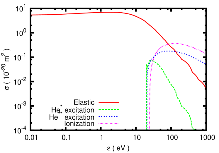
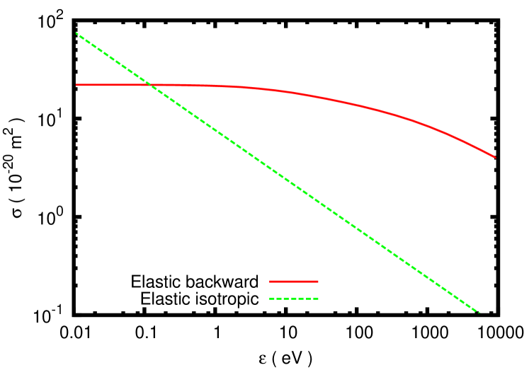
Figure 1: Cross sections for electron-neutral collisions (upper panel) and ion-neutral collisions (lower panel). The energies shown in the lower panel are expressed in the centre of mass frame.

The benchmark assumes that the plasma is composed only of electrons and helium monomer ions. Collisional processes are therefore limited to interactions between these species and neutral helium. For electron-neutral collisions, the cross section compilation known as Biagi 7.1 is used (Biagi, 2004). This consists of an elastic momentum transfer cross section, two excitation cross sections, and an ionization cross section. These cross sections assume isotropic scattering in the centre of mass frame, and are consistent with transport data when used in conjunction with such scattering. The benchmark therefore requires isotropic scattering for all electron collision processes. After an ionizing collision, the residual energy is divided exactly equally between the primary and secondary electrons. For ion-neutral scattering, we adopt the proposal of Phelps (1994), which approximates the anisotropic scattering cross section as an isotropic scattering component and a backward scattering component, both in the centre of mass frame. Such cross sections for helium have been given as analytic expressions (Phelps, 2005), which have been developed into tables for use in the present benchmark. These tables represent the cross sections as functions of the centre of mass energy. The tabulated cross sections for both electrons and ions are to be interpolated linearly whenever intermediate values are required. In the (unlikely) event that data are needed beyond the maximum tabulated energy, the last value in the table is to be substituted. Both sets of cross sections are available as electronic supplements to this paper, and are shown for reference in figure 1. Further fundamental constants are to be represented by the 2006 CODATA values (Mohr et al., 2008), expressed to at least four places of decimals.

The procedure for running the benchmarks is the following. The simulation is initialized with the conditions specified in table 1. The system is then integrated in time for the indicated interval, and an average is taken over a sub-interval at the end of the calculation. These time intervals are also specified in table 1. The average values obtained in this way are the benchmark results. In the discussion following, we focus on the ion density distribution as the primary benchmark result. This is because this quantity has an unambiguous definition in any likely simulation procedure, and is highly sensitive to both numerical effects and implementation details.

III Simulation procedure

Each of the simulation codes implements the classical particle-in-cell algorithm with Monte Carlo collisions Hockney and Eastwood (1981); Birdsall and Langdon (1991); Birdsall (1991). As is well-known, in this approach the charged particles of the plasma are represented by a set of so-called superparticles, which are much smaller in number than the physical particles. These superparticles are immersed in self-consistently generated electric fields obtained by solving Poisson’s equation in a finite difference form on a uniform spatial grid. In the conventional expression of the method, the time integration of particle trajectories uses the explicit leap-frog scheme, which is second order accurate in the time step, $\Delta t$, and the solution of the Poisson equation is second order accurate in the cell size, $\Delta x$. All the present codes use bi-linear weighting for mapping grid quantities to particle positions and vice versa (Hockney and Eastwood, 1981; Birdsall and Langdon, 1991; Birdsall, 1991). The particle-in-cell method is subject to stability and accuracy conditions. Generally accepted accuracy conditions for the cell size and time step are

$$\omega_{p}\Delta t \lesssim 0.2$$ (1)

$$\frac{\lambda_{D}}{\Delta x} \gtrsim 2,$$ (2)

where $\omega_{p}$ is the plasma frequency and $\lambda_{D}$ is the Debye length. These results are derived from extensive computer experiments (Hockney and Eastwood, 1981). Conditions 1 and 2 can be combined to form a dependent constraint

$$\frac{\Delta t}{\Delta x}\sqrt{\frac{k_{B}T_{e}}{m_{e}}}\lesssim 0.4,$$ (3)

showing that thermal electrons are displaced by much less than one cell per time step when these conditions are satisfied. There is a third numerical parameter, which controls the ratio between the superparticle density and the physical particle density. This is often called the particle weight. The particle weight is not defined uniformly by the codes employed in this study. The data given in table 1, however, implicitly specify the particle weight for all such definitions. No universal rule exists for selecting the particle weight, and indeed the evidence suggests that a wide range of values may be appropriate to different contexts (Turner, 2006), so that a “rule-of-thumb” cannot be given at present. The numerical parameters for particle-in-cell simulations given in table 1 have been chosen conservatively according to the information available, and after some experimentation. This topic will be revisited below when we discuss numerical uncertainty in the benchmark results.

Monte Carlo collisions are handled in the usual way (Birdsall, 1991; Vahedi and Surendra, 1995; Donkó, 2011), by testing for collisions once per time step. This procedure is appropriate when the collision frequency is small compared with the plasma frequency, which is the usual situation in low-pressure discharges. In general, the collision frequency for each particle species varies in some arbitrary way with relative speed. However, appreciable algorithmic simplification is achieved by adopting the so-called null collision method, in which a fictitious collision process is introduced in order to render the total collision frequency a constant for each particle species, denoted by $\nu_{e,i}$. One then has a constant collision probability per time step for each species:

$${\cal P}_{e,i}=1-\exp(-\nu_{e,i}\Delta t)\approx\nu_{e,i}\Delta t.$$ (4)

Once a particle is deemed to have collided, a second Monte Carlo step is needed to select a process. Since a particle is only permitted to collide once per time step, this procedure introduces another constraint, namely

$$\nu_{e,i}\Delta t\ll 1.$$ (5)

During a collision the momentum and energy of the particle are appropriately adjusted, and any necessary new particles are added to the simulation. Further discussion of Monte Carlo procedures for particle-in-cell simulations can be found elsewhere (Birdsall, 1991; Vahedi and Surendra, 1995; Donkó, 2011).

Each of the codes used in this study implements the basic algorithm outlined above and discussed in detail in the references. We have foregone complications that introduce additional numerical parameters and perhaps variation in implementation, such as subcycling Adam et al. (1982). Within this framework, each of the codes has been implemented independently and without consultation between the authors prior to the benchmarking exercise. Consequently, the codes differ in many details. They are implemented in different computer languages, use different data structures, are designed for different computer architectures, and doubtless differ in many other respects owing to the varied practical and philosophical views of the authors. The most salient features of the five codes we have employed are summarized in table 2. For convenience of later reference, each code has been assigned a distinguishing letter. During the course of the benchmarking, certain minor imprecisions were discovered, and these have been corrected. We think it unlikely that these would have been exposed outside the context of the present study, since the effects on the results were subtle. But these were, nevertheless, implementation errors that came to light as consequence of benchmarking. We note also that certain inconsistencies that emerged during the development of the benchmarks were traced to deficient pseudo-random number generation. This was a surprise. The detailed issues involved are not well understood by us, but we urge caution when choosing a source of random numbers.

Particle-in-cell calculations are evidently stochastic. Even in temporal equilibrium, fluctuations will occur around some average value. These fluctuations are driven by the stream of pseudo-random numbers consumed by the Monte Carlo elements in the simulation, but may also be affected by other factors, such as round-off error in finite precision arithmetic. Pseudo-random number generators typically are deterministic algorithms initialized with a seed value, yielding a different sequence of values for every unique seed. Consequently, every simulation program gives results that depend at least on the seed value. Moreover, even computers that nominally implement standard floating point arithmetic do not always respect the rounding rules strictly, with the result that the same program executed on different computers or using different software tools is likely to give different results. Consequently, for these and other reasons, we do not expect that the diverse implementations available to this study can give identical results, even for the same physical conditions and numerical parameters. We can however ask whether the results from the different codes can be statistically distinguished. We approach this problem by treating the ion densities computed at the mesh points as a set of random variables. If we can characterize the density at mesh point $j$ by an average value $\bar{n}_{i}(x_{j})$ and a standard deviation $\sigma_{i}(x_{j})$, then, for a particular set of mesh densities $n_{i}(x_{j})$ drawn from the simulation, we can compute

$$X^{2}=\sum_{j}\frac{\left[n_{i}(x_{j})-\bar{n}_{i}(x_{j})\right]^{2}}{\sigma_{i}(x_{j})^{2}}.$$ (6)

If the random variables are uncorrelated and normally distributed, and the set of values $n_{i}(x_{j})$ is actually drawn from the distribution defined by $\bar{n}_{i}(x_{j})$ and $\sigma_{i}(x_{j})$, then the value of $X^{2}$ is drawn from a well-known distribution function (Abramowitz and Stegun, 1965, sec. 26.4). If we find that the value of $X^{2}$ that we calculate is far into the tail of this probability distribution, we will conclude that the values $n_{i}(x_{j})$ were likely not drawn from the assumed distribution. By this means, we can establish whether the results of two simulation programs are statistically distinguishable or not.

There is a difficulty, in that we have no grounds for assuming that the densities at the mesh points have the properties assumed above of being uncorrelated and normally distributed. This, however, only means that the distribution of values of $X^{2}$ is not the one usually assumed. We can proceed by using one simulation to generate the values of $\bar{n}_{i}(x_{j})$ and $\sigma_{i}(x_{j})$, and the distribution of $X^{2}$ values, and we can proceed to test the other simulations against these results in the manner described above. We expect a different distribution of $X^{2}$ for each benchmark case. Fig. 2 shows the distribution functions that are determined in this way. Each has been normalized such that

$$\int_{0}^{\infty}f(X^{2})dX^{2}=1.$$ (7)

We note that the conventional $X^{2}$ distribution is characterized by the number of degree of freedom, $k$, which is in this case equal to the number of mesh points. When $k\gg 1$, the distribution of $X^{2}$ is approximately normal, with mean value $k$ and standard deviation $\sqrt{2k}$. The distributions shown in fig. 2 indeed have a mean close to $k$, but evidently have a larger standard deviation and considerable skew. We have not investigated the origin of these features, but we speculate that the cause is correlations between the density fluctuations at neighbouring mesh points, produced by plasma dynamical effects.

Our procedure, therefore, begins by generating values of $\bar{n}_{i}(x_{j})$ and $\sigma_{i}(x_{j})$, such that the standard deviation of the mean values $\bar{n}_{i}(x_{j})$ is negligible compared to the population standard deviation $\sigma_{i}(x_{j})$. We obtain these results by observing fluctuations around a stationary state in an extended calculation using code E. From this extended calculation we also find the $X^{2}$ distributions shown in fig. 2. We can then take a result from any of the other codes, compute $X^{2}$ using eq. 6, and refer to the data in fig. 2 and table 4 to determine the significance of the result. If we find no unlikely values, we can declare that the test codes indeed are statistically indistinguishable. On the sensitivity of this test, we can say that a consistent difference between two simulations results of about 0.5 % will produce a $X^{2}$ value that should occur by chance only about once in 10 000 trials. A difference of this magnitude should therefore be easily detected. On the other hand, a systematic difference of 0.1 % shifts the value of $X^{2}$ by an amount small compared to the normal ranges indicated in fig. 2 and table 4, so that a difference of this magnitude cannot be discerned.

If we were concerned to demonstrate only that the test codes give practically identical results, then we could stop here. However, we intend our results to be of value to authors of other kinds of codes than particle-in-cell codes, and for this reason we need to go a step further and estimate the numerical errors remaining in our calculations. We have done this using a refinement strategy. Since the convergence of particle-in-cell simulations with Monte Carlo collisions, as a function of the numerical parameters, has never been fully investigated (some indications are give by Vahedi et al. (1993) and Turner (2006)) , the optimal refinement procedure is not clear. Our procedure is a simple one. At each refinement, we halve the time step and the cell size. Since the algorithm is second order in these quantities, this should reduce the associated numerical errors by a factor of four. Numerical errors associated with the number of particles per Debye length, $N_{D}$, vary as $N_{D}^{-1}$ or $N_{D}^{-2}$, depending on the collisionality and nature of the error Turner (2006). To achieve a reduction of these errors by at least a factor four, then, we should increase the number of particles by a factor of four. This procedure appears reasonable, but is not guaranteed to reduce the error in the solution by a factor four, because the relationship between the velocity space diffusion effects regulated by $N_{D}$ and the global error in the solution is not clear. Nevertheless, by comparing solutions at different levels of refinement we can form some view on the magnitude of the errors.

IV Results

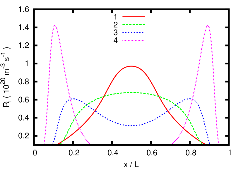
Figure 3: Time averaged ionization source term for the four benchmark cases.

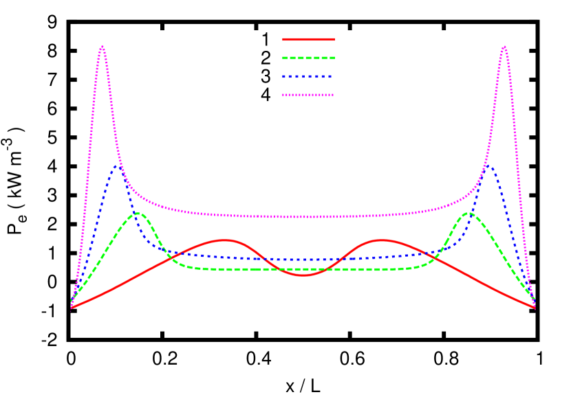
Figure 4: Time averaged power density ($\langle J_{e}\cdot E\rangle$) coupled to electrons for the four benchmark cases.

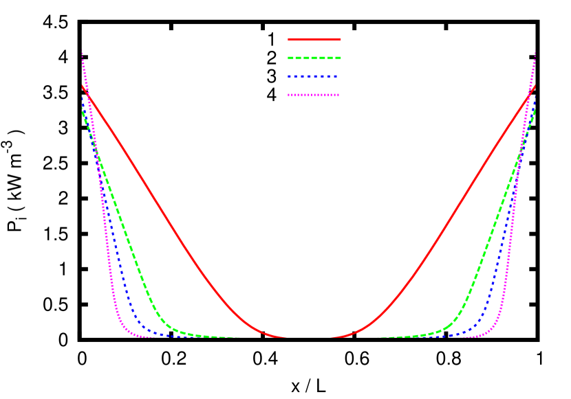
Figure 5: Time averaged power density ($\langle J_{i}\cdot E\rangle$) coupled to ions for the four benchmark cases.

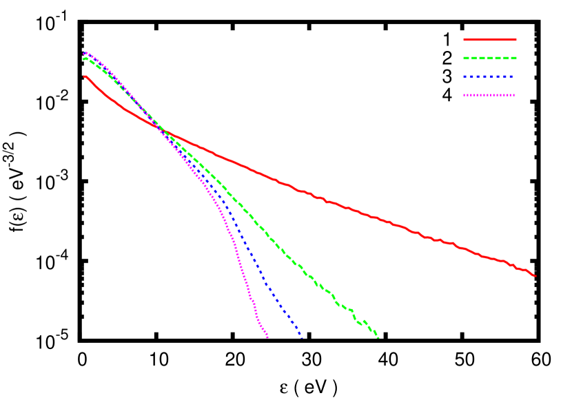
Figure 6: Time and space averaged electron energy probability functions for the four benchmark cases. These data are normalized such that $\int_{0}^{\infty}\sqrt{\epsilon}f(\epsilon)d\epsilon=1.$ A Maxwell-Boltzmann distribution would appear as a straight line on this plot.

A summary of the main physical parameters for each benchmark case, together with numerical figures of merit, is presented in table 3. These data show that the benchmark cases conservatively satisfy the conventional accuracy conditions discussed above. The first four figures show the ionization source term (figure 3), the electrical power coupled to electrons (figure 4), the electrical power coupled to ions (figure 5) and the electron energy distribution functions for each of the cases (figure 6). We see that as the pressure increases from case 1 to case 4, both ionization and power transfer become increasingly concentrated in the sheath region. Much of this behaviour is determined by the electron energy relaxation length. For electrons below the threshold for inelastic processes, the energy relaxation length is large compared with the electrode spacing in all four cases. Consequently, we expect that the gross electron mean energy varies rather little in space. Above the inelastic threshold, however, the energy relaxation length is larger than the electrode separation in case 1, but smaller in case 4. Hence we find that in case 4, power absorption and dissipation have become more locally balanced, with maxima in the sheath regions. The electron energy distribution functions shown in figure 6 exhibit no striking structures. At the lowest pressure, the distribution function is close to Maxwellian, but at higher pressure there is an increasing depression of the high energy tail caused by inelastic collisions. None of these distribution functions shows in a marked form any of the more exotic structures that are sometimes seen, such as bumps, holes or super-thermal high energy tails (Godyak and Piejak, 1990; Godyak et al., 1992b, a; Turner and Hopkins, 1992). These features are commonly symptomatic of strongly non-local interactions between the electrons and the fields. The absence of such interactions means that simplified models using approximate treatments of the electron kinetics have a reasonable chance of reproducing the present benchmarks with tolerable accuracy.

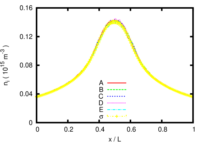
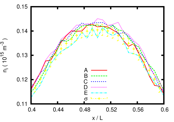
Figure 7: Ion density distribution for case 1. The curves labelled A to E show the results obtained by the indicated code. The points with error bars show the standard deviation obtained from an extended calculation using code E.

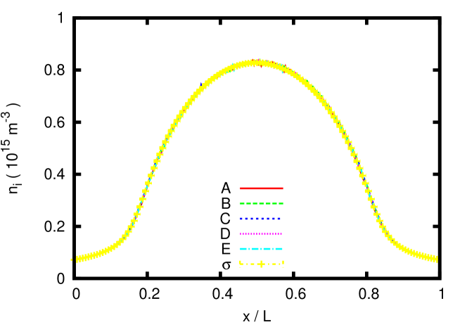
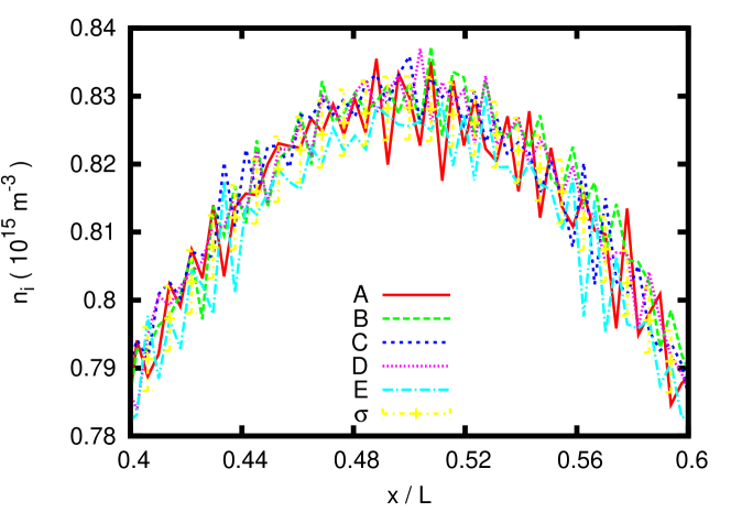
Figure 8: Ion density distributions for case 2. Refer to the caption of fig. 7 for further explanation.

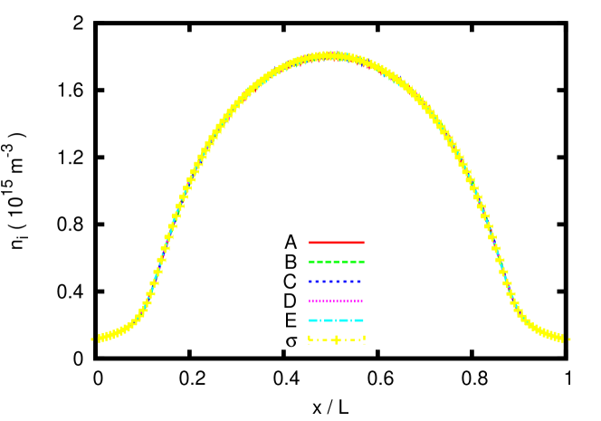
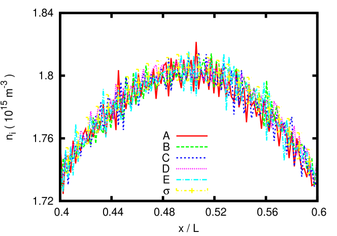
Figure 9: Ion densities distributions for case 3. Refer to the caption of fig. 7 for further explanation.

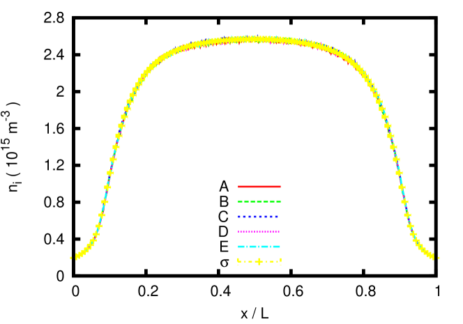
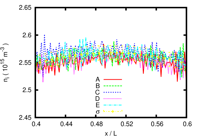
Figure 10: Ion density distributions for case 4. Refer to the caption of fig. 7 for further explanation.

In the next group of figures we present the comparisons between the ion densities for the four benchmark cases. Figures 7, 8, 9 and 10 compare the densities calculated using each of the five codes. Of course, the densities in each code fluctuate around some mean value, and we also show in these figures error bars which denote one standard deviation of this fluctuation. All the figures show a global view of the data, and an expanded region around the discharge mid-plane. From the global view, the agreement between the codes is evidently excellent, in the sense that no disagreement within the error bars can be discerned. This is also true of the expanded view, where the size of the fluctuations is more clearly evident. As we have suggested above, the coincidence of the codes can be examined objectively using a statistical test. The results of these statistical tests are summarized in table 4. We note that since code E was used to generated the $X^{2}$ distributions, the results for that code are presented essentially as a methodological test. These data can be examined in conjunction with the distributions shown in figure 2, but for convenience we have shown in the table the range of values that can be accepted as being likely to have occurred by chance. One of the twenty values shown here is outside the 95 % confidence limits, which is of course the expected outcome.

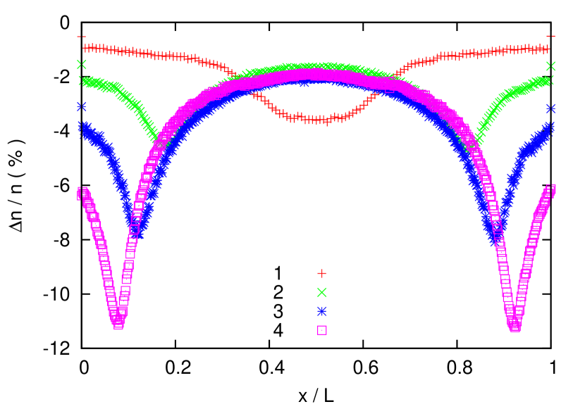
Figure 11: Estimation of the residual numerical errors in each of the four benchmark cases. These data have been obtained by comparing the base cases with additional calculations using substantially more refined numerical parameters. Since we have compared the solutions at coincident mesh points, this presentation overstates the significance of the errors where there are strong spatial gradients (c.f, figures 7,8,9 and 10).

The evidence we have shown above strongly suggests that the codes under discussion are statistically indistinguishable, and from this result we wish to urge the conclusion that the codes are also correct in some usefully strong sense. Of course, the basis for this claim is the assumption that five independently developed codes are unlikely to be united in error. Even if this is so, the benchmark results obtained from these codes have an accuracy that is limited by numerical effects arising from finite time steps, cell sizes and particle density. Figure 11 shows evidence relevant to the question of estimating the size of this residual error. As we explained above, we have approached this issue using a sequence of computations with increasingly refined numerical parameters. In each case, the most refined solution has the cell size and time step reduced by a factor four, and the number of particles increased by a factor sixteen, for an increase in numerical exertion by a factor of about sixty four. By comparing intermediate stages in the refinement process, we estimate that the numerical uncertainty is reduced by a factor of approximately ten in the most refined solutions, relative to the base cases detailed in table 1. In figure 11 we show the difference between the base case solutions and the most refined solutions. As we note in the figure caption, we have compared the solutions at coincident spatial points, and this procedure leads to apparently large errors in regions where there are strong spatial gradients. A more significant estimator of the error in each solution is the difference in the mid-plane, which is seen to be rather uniformly a few percent. The error in the refined solutions is approximately ten times smaller than this. These data provide some guidance to authors of simulation codes other than particle-in-cell codes as to whether their results are consistent with the benchmark or not

V Discussion

The results obtained in the present work are appreciably more consistent than those found in the earlier benchmark comparison of Surendra (1995). For example, results from the three particle-in-cell implementations considered in that exercise were typically different by $\sim$5 %, and differences in excess of 15 % occurred. Larger divergences were found between the particle-in-cell simulations and other kinetic solvers—as much as 100 % in some cases. The range of all the simulations considered spanned approximately a factor of two in electron temperature and a factor of three in density. On the evidence available, these differences are not easy to understand—but the kinetic simulations, at least, are all supposedly solving the same physical model, so we must assume either implementation error or operator error (i.e. inappropriate physical or numerical parameters). As evidence from other fields shows, errors of these types occur commonly, and are difficult to eliminate. In the present work, we cannot claim with certainty that we have eradicated all such mistakes, but we can make a limited claim based on the statistical arguments presented above: Any remaining errors affect the results systematically by appreciably less than 1 %. The residual numerical errors in the base cases are significantly greater than this, so we have also provided data using more refined numerical parameters that reduce the overall precision to about the 1 % level. These data provide a basis for authors of other simulation codes to evaluate the accuracy of their own results, which of course is one of our central aims.

A precision much better than 1 % is perhaps of limited practical value. In the end, the primary purpose of simulations is to predict the outcome of experiments, and not many relevant experiments (if any) approach an accuracy of 1 %. Moreover, the accuracy of the simulations is limited by the available physical data as well as by numerical considerations. The most accurate cross section data available at present probably have an uncertainty of at least a few percent. The base case numerical parameters shown in table 1 therefore probably entail an appropriate level of numerical exertion for most purposes. Indeed we note that the difference between the present benchmark results and comparable experiments (Godyak et al., 1992b, a) is far larger than any reasonable estimate of the error due to numerical effects or faulty cross section data—roughly a factor of two in density and voltage, for a given current density. We assume that this is due to an incomplete physical model. For example, we have neglected emission of particles from electrodes and all effects of excited states (Hitchon et al., 1993). This topic will be further explored in future work.

Although the principal aim of the benchmarks that we present here is to facilitate verification of codes, we note that a secondary objective can be achieved, and this is to compare the performance of different implementations. The interest of this activity is increased by knowing that the codes are performing the same calculation (within some tolerance, at least) so that any difference in execution time is due to hardware and implementation strategy. The codes under investigation take different approaches. Code C, for example, is implemented in MATLAB, a high level language that generally favours ease of programming over efficiency. Codes A and D are traditional implementations in the C language, and as such similar in concept to the well-known PDP1 (Verboncoeur et al., 1993). Codes B and E both target features of modern computer architectures such as multi-threaded execution, symmetric multi-processing, and vectorisation. These are, relatively speaking, complex implementations aiming at high performance. Developing a basis for verifying such codes was a major motivation of the present work. On the benchmark cases discussed here, codes B and E perform comparably, and are each about a factor of twenty faster than the serial codes A and D, which are themselves about twice as fast as the MATLAB code C. These differences are of considerable practical significance. For example, when all the calculations are carried out using reasonably modern desktop computers, benchmark 4 takes approximately six hours to execute using codes B and E, but almost three weeks using code C.

VI Concluding Remarks

Our aim in this work was to develop benchmarks for low-temperature plasma physics simulations. We approached this problem by specifying four benchmark cases, each with comprehensively defined physical and numerical conditions. We have then shown that five independently developed particle-in-cell simulations produce results for these benchmarks that are indistinguishable on a statistical basis. A more precise statement would be that the implementation uncertainty is less than 0.5 %. We proceeded to investigate the numerical uncertainty in the benchmark results, and we have presented a second set of benchmark results in which the numerical uncertainty is reduced to approximately the same level as the implementation uncertainty. Thus we claim that these latter results have an uncertainty at about the 1 % level. We do not think that there is any advantage in attempting to further refine these results at the present time, allowing for the uncertainty in both basic data and experimental characterization. Our intention is that these data can be used by developers of particle-in-cell codes to verify their work in a rather rigorous fashion, using the statistical procedures that we have discussed, while authors of codes based on other principles can evaluate the accuracy of their work by less formal methods.

Of course, the present benchmarks exercise only a subset of the features likely to be desired in comprehensive simulation packages. For example, we have not treated multi-dimensional effects or electro-magnetic effects, and plasma chemistry only in a limited fashion. Nevertheless, we think that the methodology we have developed represents a powerful platform for future developments encompassing these more advanced aspects.

Physical parameters
			1	2	3	4
Electrode separation	$L$	( cm )	6.7
Neutral density	$N$	( 1020 m-3 )	9.64	32.1	96.4	321
Neutral temperature	$T_{n}$	( K )	300
Frequency	$f$	( MHz )	13.56
Voltage	$V$	( V )	450	200	150	120
Simulation time	$t_{S}$	( s )	$1280/f$	$5120/f$	$5120/f$	$15360/f$
Averaging time	$t_{A}$	( s )	$32/f$	$32/f$	$32/f$	$32/f$
Physical constants
			1	2	3	4
Electron mass	$m_{e}$	( 10-31 kg )	9.109
Ion mass	$m_{i}$	( 10-27 kg )	6.67
Initial conditions
			1	2	3	4
Plasma density	$n_{0}$	( 1014 m-3 )	2.56	5.12	5.12	3.84
Electron temperature	$T_{e}$	( K )	30 000
Ion temperature	$T_{i}$	( K )	300
Particles per cell	$N_{C}$		512	256	128	64
Numerical parameters
			1	2	3	4
Cell size	$\Delta x$	( m )	$L/128$	$L/256$	$L/512$	$L/512$
Time step size	$\Delta t$	( s )	$(400f)^{-1}$	$(800f)^{-1}$	$(1600f)^{-1}$	$(3200f)^{-1}$
Steps to execute	$N_{S}$		512 000	4 096 000	8 192 000	49 152 000
Steps to average	$N_{A}$		12 800	2 5600	51 200	102 400

Table 1: Physical and numerical parameters for the benchmarks

Code	Author(s)	Language	Architecture
A	Derzsi and Donkó	C	CPU
B	Eremin	C for CUDA	GPU
C	Lafleur	MATLAB	CPU
D	Mussenbrock	C	CPU
E	Turner	C	CPU (multithreaded)

Table 2: Summary characteristics of the five simulation programs employed in this study.

Physical characteristics
	1	2	3	4
$n_{i}$ ( 1015 m-3 )	0.140	0.828	1.81	2.57
$k_{B}T_{e}$ ( eV )	9.36	4.69	3.95	3.65
$S_{e}$ ( W m-2 )	34.3	51.6	85.2	193
$S_{i}$ ( W m-2 )	90.6	43.3	32.0	27.1
$J_{i}$ ( A m-2 )	0.219	0.215	0.195	0.186
Numerical characteristics
	1	2	3	4
$\omega_{p}\Delta t$	0.121	0.150	0.110	0.066
$\lambda_{D}/\Delta x$	3.72	2.14	2.66	2.14
$\nu_{e}\Delta t$	0.0158	0.0262	0.0391	0.0643
$\nu_{i}\Delta t$	0.00688	0.0114	0.0171	0.0283
$N_{D}$	1042	886	1204	917
$N_{P}$	31900	118000	283000	329000

Table 3: Physical and numerical characteristics for the four benchmark cases. In the upper section of the table, $n_{i}$ and $T_{e}$ are the ion density and electron temperature in the mid-plane of the discharge, $S_{e}$ and $S_{i}$ are the line integrated electrical power coupled to electrons and ions, respectively, and $J_{i}$ is the ion current collected at either electrode. All these quantities are time averaged. The lower table shows numerical figures of merit, which are evaluated at the mid-plane of the discharge using time averaged data, apart from the total number of particles $N_{P}$, which figure refers to the entire discharge volume.

	1	2	3	4
A	240	199	540	606
B	192	310	503	543
C	328	408	503	703
D	242	209	425	517
E	57	219	592	542
95%	55–303	177–435	405–693	417–665
99%	48–405	160–548	382–798	392–730

Table 4: $X^{2}$ values for each of the simulation programs applied to each of the benchmark cases. The lines at the bottom of the table show the ranges of values that encompass 95 % and 99 % of the area under the distributions shown in figure 2.

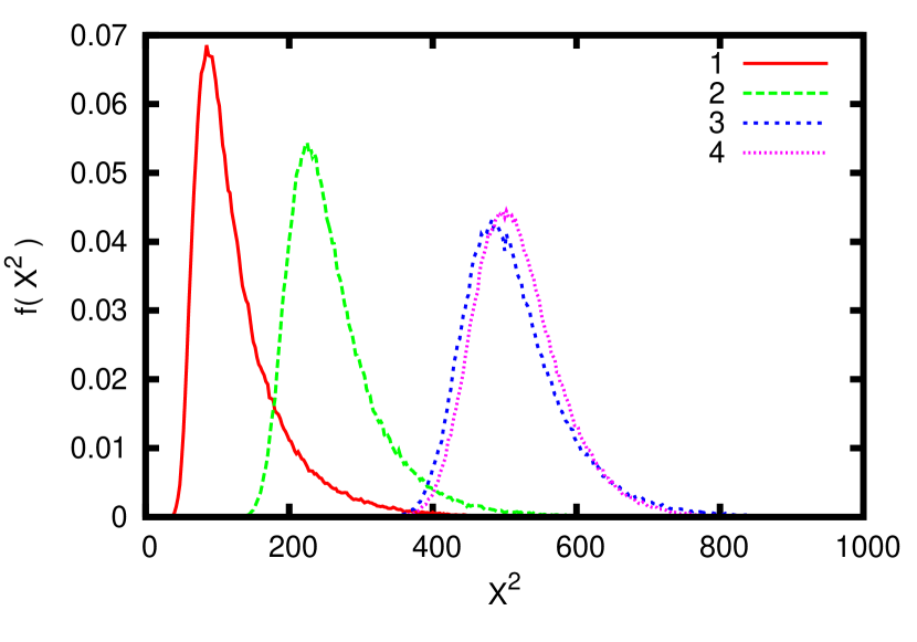
Figure 2: Distribution of $X^{2}$ values for the four benchmark cases

Appendix A Moment models

In this appendix we simulate the benchmark conditions using a moment model, and we compare the data so obtained with the particle-in-cell simulation results presented above. A moment model is based a greatly simplified physical model. Instead of calculating the phase space distribution functions of the particles, as a particle-in-cell simulation does, a moment model solves conservation equations for a limited number of macroscopic physical quantities, such number density, momentum, and thermal energy. These equations incorporate a set of rate constants and transport coefficients, which are in principle dependent on the energy or speed distributions of the particles. Moreover, the moment equations are themselves developed by computing velocity space moments of the Boltzmann equation, and this procedure leads in principle to an infinite set of mutually coupled partial differential equations. If we solve for only the first two or three moments (as implied above) then this hierarchy of equations must be truncated by some means—the so-called “closure problem.” So although a solution of the moment equations is computationally economical, compared to solving the Boltzmann equation, there is considerable underlying theoretical complexity. Indeed most moment models include informally developed elements, such as transport and rate coefficients injected from a Monte Carlo simulation, a Boltzmann equation solution, or experimental data. There may also be differences in detail on the formulation of the moment equations themselves, the implementation of boundary conditions and the choice of numerical procedure. How the many decisions involved in designing a moment model affect the accuracy of the results is not well understood, and this is an issue that benchmarking can address. Our intention here, however, is more modest. We aim only to offer an example of applying a moment model to the benchmark cases described in the main text. The moment model that we have employed is a commercial one, offered by COMSOL Multiphysics (COMSOL, 2012). In most respects, this is a conventional formulation, calculating three moments for electrons and two for ions. An unusual feature is that the species densities are expressed in a logarithmic form—details of this aspect and others are to be found in documentation for the package, and will not be discussed here. For electrons, rate constants and transport coefficients were computed from the cross sections specified above using BOLSIG+ (Hagelaar and Pitchford, 2005), while the ion mobility $\mu_{i}$ was expressed using the result given by Patterson (1970) for a gas temperature of 300 K:

$$\mu_{i}N=2.69\left[1+1.2\times 10^{-3}(E/N)^{2}+4.2\times 10^{-8}(E/N)^{4}\right]^{-\frac{1}{8}}$$ (8)

where $E/N$ is expressed in Td. This result is in reasonable agreement (within 5 % over the range 1 Td $<E/N<900$ Td) with Monte Carlo transport calculations using the ion scattering cross sections given above. Naturally, the numerical parameters specified for the particle-in-cell simulations are inapplicable to the moment model, which has different stability and accuracy conditions.

Comparisons between these moment calculations and the particle-in-cell simulation data are shown in figure 12. In general, there is qualitative agreement concerning the spatial distribution of the ion density, but disagreement about the maximum density. Perhaps surprisingly, this disagreement increases with neutral gas pressure, and is about 50 % in case 4. Such variations cannot reasonably be attributed to numerical effects, and we assume that modelling issues are in play, such as the procedure for computing rate and transport coefficients, use of the drift-diffusion approximation, etc. The trend of these differences is generally similar to observations in the earlier benchmark of Surendra (1995), where the moment models generally gave smaller densities than the particle-in-cell simulations. A more comprehensive enquiry would be of interest. This is beyond the scope of the present study, but may be the subject of future work.

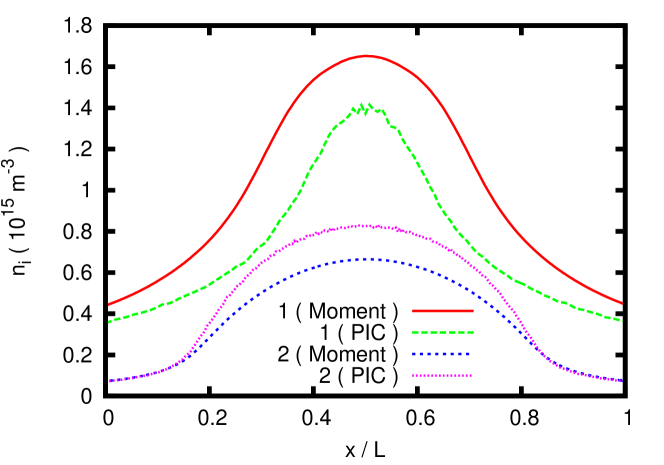
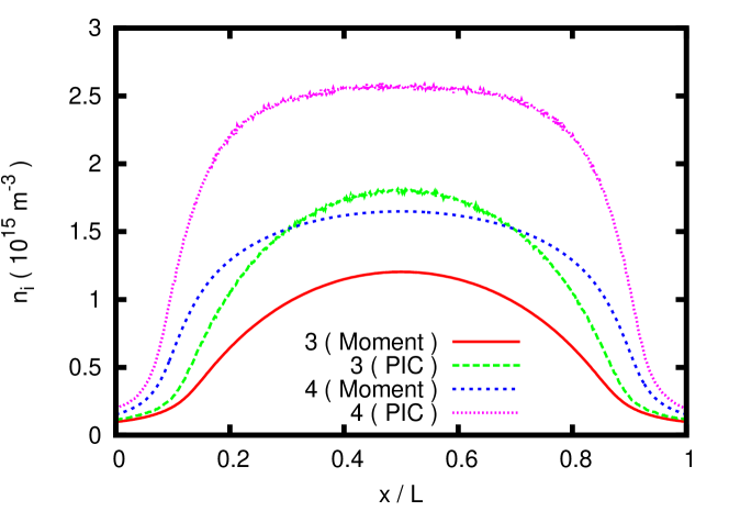
Figure 12: Comparison of the moment model computations described in A with the particle-in-cell calculations of the main text. The top panel shows benchmark cases 1 and 2, with the data for case 1 scaled by a factor of ten for clarity of presentation, and the bottom panel shows benchmark cases 3 and 4.