Analysis on Correlations between Subsurface Kinetic Helicity and Photospheric Current Helicity in Active Regions

Abstract

An investigation on correlations between photospheric current helicity and subsurface kinetic helicity is carried out by analyzing vector magnetograms and subsurface velocities for two rapidly developing active regions. The vector magnetograms are from the SDO/HMI (Solar Dynamics Observatory / Helioseismic and Magnetic Imager) observed Stokes parameters, and the subsurface velocity is from time-distance data-analysis pipeline using HMI Dopplergrams. Over a span of several days, the evolution of the weighted current helicity shows a tendency similar to that of the weighted subsurface kinetic helicity, attaining a correlation coefficient above 0.60 for both active regions. Additionally, there seems to be a phase lag between the evolutions of the unweighted current and subsurface kinetic helicities for one of the active regions. The good correlation between these two helicities indicate that there is some intrinsic connection between the interior dynamics and photospheric magnetic twistedness inside active regions, which may help to interpret the well-known hemispheric preponderance of current-helicity distribution.

1 Introduction

Parker (1955) initiated a model for the cycle of magnetic field in the sun with a mechanism named “cyclonic motion”, and Steenbeck et al. (1966) established the feasibility of AC or DC dynamos in astrophysical environment. At that time, they formulated a consistent explanation of the role of the cyclonic motions, which was later called $\alpha$-effect (e.g., Roberts & Stix, 1971). Pouquet et al. (1976) suggested that turbulence and magnetic fields were common features of many celestial bodies and the $\alpha$-effect contained both the kinetic and magnetic helicity. The correlation between these two kinds of helicities has been under debate (e.g., Brandenburg et al., 1990, 1995). Keinigs (1983) gave an example of $\alpha$-effect including zero kinetic helicity and the $\alpha$-effect relied on the ensemble average of fluctuating velocity and magnetic field. That is to say, the generation of magnetic field requires current helicity but not necessarily the kinetic helicity. The $\alpha$-effect is central to dynamo theory and magnetic field generation, however, it lacked observational and experimental supports over a long term (Sokoloff, 2007). Not until the recent 20 years, mirror asymmetries of magnetic field (magnetic helicity) (Seehafer, 1990; Pevtsov et al., 1995; Bao & Zhang, 1998; Hagino & Sakurai, 2004; Zhang et al., 2010) and the velocity (kinetic helicity) (Zhao & Kosovichev, 2003) were found in observations. Apparently, frozen flow with the magnetic field in the fluid of high magnetic Reynold number is a necessary condition for the $\alpha$-effect in the framework of Parker’s dynamo model. It can be easily inferred that the variation of kinetic and current helicity in the fluid might be a good manifestation of the freezing process. Although the speculation of the depth of $\alpha$-effect is still under debate, it is expected that some relevant characteristic might be captured even near the photosphere.

Local helioseismology provides a unique tool to determine the sub-photospheric flows of active regions. A statistical study by Zhao (2004) showed that the subsurface kinetic helicity inside active regions observed by the Solar Heliospheric Observatory / Michelson Doppler Imager (SOHO/MDI) observations seemed to have a hemispheric preponderance, like what magnetic (or current) helicity observations had shown (Pevtsov et al., 1995; Bao & Zhang, 1998). Gao et al. (2009) analyzed the connection between the photospheric current helicity, calculated from vector magnetograms observed by Huairou Solar Observing Station, and the subsurface kinetic helicity measured from MDI observations in 38 solar active regions. Although there was an opposite hemispheric trend between the sign of current helicity and that of subsurface kinetic helicity near the solar surface, the result did not support that the subsurface kinetic helicity had a cause and effect relation with the photospheric current helicity at the depth of 0-12 Mm. Similar result was reported by Maurya et al. (2011) as well.

Now, Solar Dynamics Observatory / Helioseismic and Magnetic Imager (SDO/HMI; Scherrer et al., 2012; Schou et al., 2012) observations provide an unprecedented opportunity to investigate the connection between subsurface kinetic helicity and current helicity, as both subsurface flow velocity and photospheric vector magnetic field are available at the same time. Subsurface kinetic helicity can be computed from subsurface flow velocities, which are routinely processed through the HMI time-distance analysis pipeline (Zhao et al., 2012). Photospheric current helicity is able to be computed from the photospheric vector magnetograms (Hoeksema et al., 2012). In this Letter, we focus our study on active regions NOAA AR 11158 and AR 11283, both of which have continuous observational coverage that allows us to investigate the relationship between subsurface kinetic helicity and current helicity over a longer period rather than just a snapshot comparison as done in our previous study (Gao et al., 2009). In §2, we describe the procedure of observation and data preparation for this analysis, and present our results in §3. We then summarize and discuss our results in §4.

2 Observation and Data Reduction

HMI observes the full-disk Sun continuously, providing Doppler velocity and line-of-sight magnetic field, among others, with a 45-sec cadence, and also vector magnetic field with a cadence of 12 min (Schou et al., 2012). Each full-disk image has 4096 $\times$ 4096 pixels with a spatial resolution of 0.504 arcsec pixel^-1 (i.e., approximately, 0.03 heliographic degree pixel^-1 at the solar disk center). Subsurface flow velocities are computed from HMI Doppler-shift observations using time-distance helioseismology data-analysis pipeline (Zhao et al., 2012). In practice, to execute this data-analysis pipeline, users provide the Carrington coordinate for the interested area and time of the interested period, then the pipeline code selects an area of roughly $30^{\circ}\times 30^{\circ}$ centered at the given coordinate, and a duration of 8 hours with the given time as the middle point. Normally, the pipeline generates a subsurface flow field consisting 256 $\times$ 256 pixels with a horizontal spatial sampling of 0.12^∘ pixel^-1, and a number of depths covering from the photosphere to 20 Mm in depth. We performed analysis in all depths, and found that the shallowest depth, i.e., 0 – 1 Mm, gave the most consistent and robust results. Thus, in this Letter, we only present results obtained from this depth and leave analyses of deeper layers for future studies. And also, a recent comparison of subsurface flow field at the depth of 0 – 1 Mm, obtained from this time-distance data-analysis pipeline, and photospheric flows obtained from the DAVE4VM technique (Schunk, 2008) found a reasonable agreement in horizontal flow fields inside active regions (Liu & Zhao, 2012). Vector magnetograms are also from HMI observations, and these data have also been widely used in carrying out quantitative analysis (e.g., Sun et al., 2012).

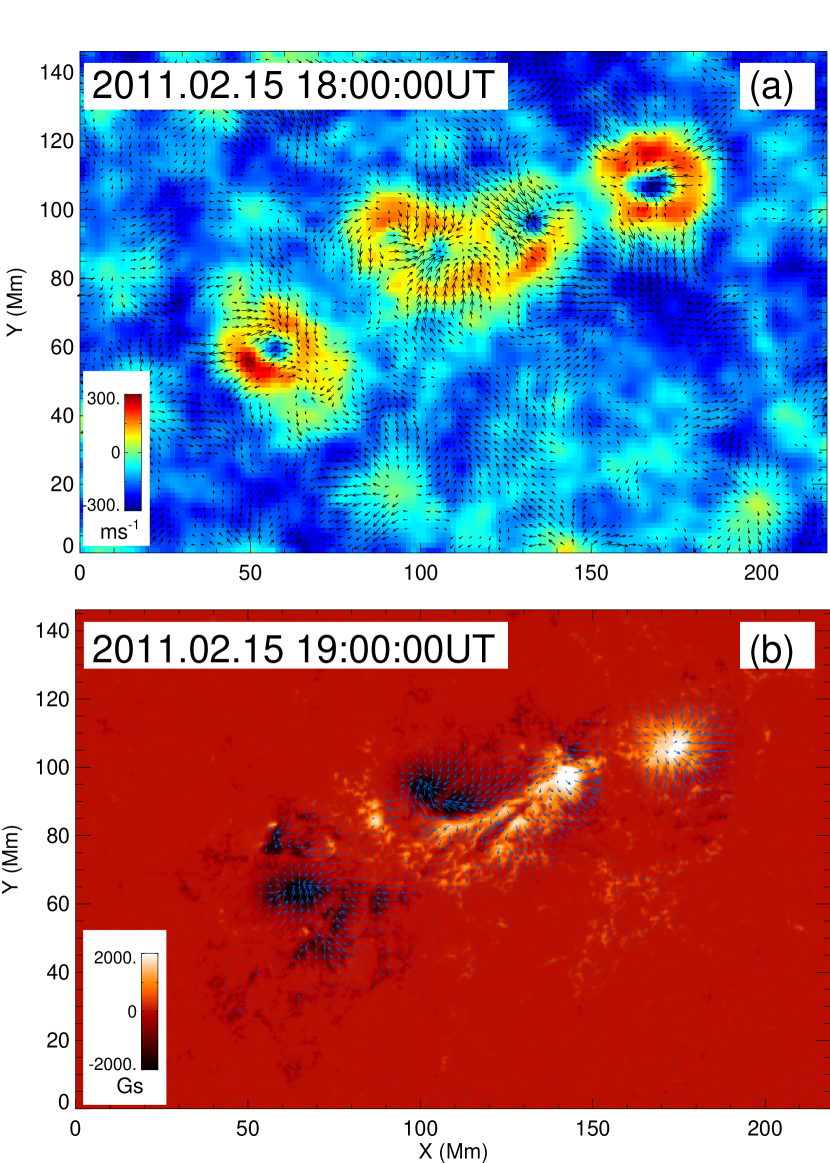
Figure 1: (a) Example of subsurface velocity field of NOAA AR 11158 at a depth of 0 – 1 Mm. Background shows the vertical component of the velocity and arrows show the horizontal components. The maximum vertical velocity is 285 m s^-1 and the longest arrow represents a horizontal speed of 441.8 m s^-1. The spatial sampling of the vertical component is 2.016^′′$\times$2.016^′′, and the field of view is 3.02^′$\times$2.02^′. (b) Example of vector magnetogram of NOAA AR 11158, with white showing positive polarity and black showing negative. The longest arrow represents a transverse field of 2356 G, and the transverse field lower than 300 G is not shown.

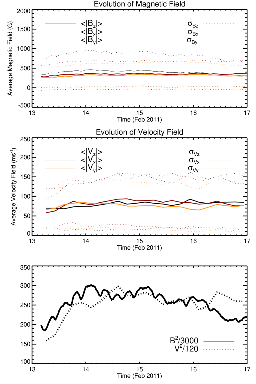
Figure 2: Temporal evolution of the three components of the magnetic field (top), the three components of the subsurface velocity field (middle) and the square of magnetic field and velocity (bottom).

NOAA AR 11158 was a rapidly developing active region, in which an X 2.2 solar flare started at 01:44 UT and peaked at 01:56 UT of 2011 February 15. This active region, as well as the X-class solar flare that occurred in it, were widely studied for different purposes (e.g., Sun et al., 2012; Jing et al., 2012; Liu & Zhao, 2012). Figure 1a shows an example of velocity field of AR 11158 at the depth of 0 – 1 Mm, with the background showing the vertical component of the flow and arrows showing the horizontal components. Figure 1b shows an example of vector magnetogram of NOAA 11158 taken at a time similar to the subsurface flow field. Figure 2 shows the evolution of the averaged absolute values of three components of the magnetic field and three components of the subsurface velocity, respectively. It can be found that the magnitudes of the components of the velocity and magnetic field remain relatively stable, and there is no coherent or sudden change for any of these quantities. Meanwhile, the fluctuations of these quantities are also small, as shown in the curves of standard deviations.

Another active region, NOAA AR 11283, is also studied. This region was very flare productive, generating two C-class solar flares from 22:00 UT to 23:33 UT on 2011 September 5, an X2.1 flare that started at 22:12 UT and peaked at 22:20 UT on September 6, an X1.8 flare that started at 22:32 UT and peaked at 22:38 UT, and an M6.7 flare on September 8 when the region was close to the west limb. As shown in §3, the same analysis on evolutions of photospheric current helicity and subsurface kinetic helicity is applied on both AR 11158 and AR 11283, and similar results are achieved for both active regions.

3 Results

The main purpose of this work is to study whether there is a correlation between the photospheric current helicity and subsurface kinetic helicity inside active regions. Current helicity is defined as: $H_{c}=\mathbf{B}\cdot(\nabla\times\mathbf{B})$. Similar to what was employed by Bao & Zhang (1998), the averaged value of the vertical component density of the current helicity, denoted as $\langle H_{c}^{z}\rangle$, was used in this study. In addition, we also compute the weighted $\langle H_{c}^{z}\rangle$, defined as $\langle H_{c}^{z}\rangle$ divided by the total magnetic field strength, i.e., $\langle H_{c}^{z}\rangle/|\mathbf{B}^{2}|$. This parameter has the same dimension as the mean twist $\alpha$, a commonly used proxy of magnetic helicity. However, $\alpha$ is defined as the curl of transverse magnetic field dividing the corresponding longitudinal field, hence carries a same sign as the weighted $\langle H_{c}^{z}\rangle$. Similarly, kinetic helicity is defined as $H_{k}=\mathbf{v}\cdot(\nabla\times\mathbf{v})$, and we take the averaged value of its vertical component, $\langle H_{k}^{z}\rangle$, and the value weighted by the speed, $\langle H_{k}^{z}\rangle/|\mathbf{v}^{2}|$, for further studies. To compute both values of $\langle H_{c}^{z}\rangle$ and $\langle H_{k}^{z}\rangle$, we only use the areas where $|B_{z}|>50$ Gs, and this is a popular approach taken in many previous studies, e.g., Bao & Zhang (1998). The magnetograms are rebinned to the same resolution of the velocity map, and all quantities are averaged over the same spatial areas. In this Letter, we study the evolutionary relationship between $\langle H_{c}^{z}\rangle$ and $\langle H_{k}^{z}\rangle$ inside the two flare-productive active regions introduced above.

The top panel of Figure 3 shows evolutions of the weighted current-helicity density and weighted kinetic-helicity density obtained at a depth of 0 – 1 Mm for AR 11158. The time series from 2011 February 13 to 17 are analyzed. The weighted current-helicity density with a 12-min cadence is averaged over a 4-hr period in order to compare with the weighted kinetic-helicity density, which is computed from the subsurface velocity obtained from an 8-hr data sequence with a 4-hr time step. Error bars are plotted for the current helicity with corresponding standard deviations. The two helicity curves show very similar varying tendencies and the correlation coefficient attains 0.67. Furthermore, we separate the data series into two sections. For the decreasing phase before 06:00UT of 2011 February 14, the correlation coefficient between the kinetic-helicity density and the current-helicity density is as high as 0.84. But for the rising phase after 06:00UT of 2011 February 14, the correlation coefficient drops to 0.52. The decrease of the correlation may be related to the X2.2 flare event that occurred at 01:44 UT of 2011 February 15. For the calculation of these correlation coefficients, the included data points n (correlation coefficients r) are 22 (0.67), 7 (0.84), and 15 (0.52), thus the degrees of freedom are 20, 5, and 13, respectively. The corresponding critical values of the Pearson correlation coefficients for a significance level of 0.95 are 0.423, 0.754, and 0.514, respectively. Therefore, the correlation coefficients from our calculations are all highly significant.

The bottom panel of Figure 3 shows the evolutions of the unweighted current-helicity density and unweighted subsurface kinetic-helicity density. Different from the similar evolutionary tendency of the weighted parameters, the two unweighted parameters seem to evolve out of phase. As shown in this panel, the unweighted kinetic helicity seems to have a decreasing phase about 8 hr earlier than that of the current helicity before 10:00 UT of February 14, and have an increasing phase about 4 hr behind that of the current helicity after 18:00 UT of February 14. The bottom panel of Figure 2 shows the evolution of $B^{2}$ and $v^{2}$. These two quantities seem to evolve out of phase at the beginning and more in phase after mid-day of February 14. This may account for the evolutionary difference in the weighted and unweighted kinetic helicty.

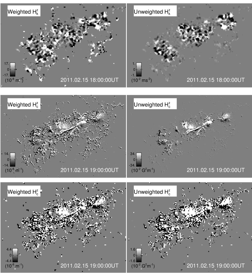
Figure 4: Snapshots showing weighted $\langle H_{k}^{z}\rangle$ (upper left) and unweighted $\langle H_{k}^{z}\rangle$ (upper right) at 18:00 UT of 2011.02.15, weighted $\langle H_{c}^{z}\rangle$ (Middle left) and unweighted $\langle H_{c}^{z}\rangle$ (Middle right) at 19:00 UT of 2011.02.15 with original spatial resolution, and weighted $\langle H_{c}^{z}\rangle$ (Bottom left) and unweighted $\langle H_{c}^{z}\rangle$ (Bottom right) after binning down to match the spatial resolution of $\langle H_{k}^{z}\rangle$. The parameters are displayed relative to the corresponding standard deviations, and color bars at the left lower corner of each panel show this scale.

The snapshots in Figure 4 show maps of the weighted and unweighted $\langle H_{k}^{z}\rangle$ as well as the weighted and unweighted $\langle H_{c}^{z}\rangle$ for some selected periods. It can be found that both of the kinetic-helicity parameters are more fragmented than the current-helicity parameters, but there is not clear correspondence between the sign distributions of the kinetic helicity and the current helicity. Besides, we also plot weighted $\langle H_{c}^{z}\rangle$ and unweighted $\langle H_{c}^{z}\rangle$ after binning down to match the spatial resolution of $\langle H_{k}^{z}\rangle$. Furthermore, we compute the correlation between the maps of weighted (unweighted) current and kinetic helicity with the same resolution. The values are 0.019 and 0.028 respectively.

For the other active region NOAA AR 11283, the evolutions of both current helicity and subsurface kinetic helicity, both weighted and unweighted, are shown in Figure 5. Similar to the results for AR11158, the evolutionary curves of the weighted parameters have a better correlation, which is 0.62 for this case, than those of the unweighted parameters. However, for the unweighted parameters, we do not see the phenomenon of that the subsurface kinetic helicity evolves ahead of the current helicity before the flare and behind the current helicity after the flare, like what is observed in AR 11158. The evolution of $B^{2}$ and $v^{2}$ for this active region does not show any phase lag either.

4 Discussion

We have studied the correlation between the evolutionary curves of the current-helicity density, computed from HMI vector magnetic field, and the subsurface kinetic-helicity density, computed from subsurface velocity field obtained from HMI time-distance data-analysis pipeline, for two flare-productive active regions. For the weighted helicities, we find that the evolution of the current helicity and subsurface kinetic helicity has a high correlation, larger than 0.60 for both active regions. But for the unweighted case, essentially, both helicities do not show a high correlation for the studied period for both regions. It is not clear why the weighted parameters show a high correlation while the unweighted parameters do not. Still, it is very interesting to see the weighted helicities attain a high correlation during the evolution of both active regions, especially when considering that these two helicities are calculated from very different data. Although the original observations were both from the same instrument HMI, current helicity is calculated from vector magnetic field which was derived from the 12-min-cadence Stokes parameters, and the subsurface kinetic helicity is calculated from the 45-sec-cadence Dopplergrams after some very complicated helioseismological processing. The high correlation between these two helicities indicate there are indeed some intrinsic connections between the subsurface kinetic helicity and the photospheric current helicity.

Since the hemispheric preponderance of magnetic (or current) helicity was reported (e.g., Pevtsov et al., 1995; Bao & Zhang, 1998), many efforts have been made to explain this observational phenomenon based on the solar dynamo (e.g., Kleeorin, 2003; Choudhuri et al., 2004; Zhang et al., 2006, 2012), and the $\Sigma$-effect of emerging magnetic flux (Longcope et al., 1998). The adopted velocity field here mainly comes from the region near the solar surface, so the correlation between the short time scale variations of kinetic and current helicity may be suitable to be explained by using the $\Sigma$-effect. The $\Sigma$-effect suggested that during the rising of the magnetic flux from convection zone to the photosphere, the large-scale writhing and the local-scale twisting together shape the tilt angle and magnetic (or current) helicity distributions of active regions. The subsurface kinetic helicity used in our analysis is presumably corresponding to the twisting inside active regions in the upper convection zone. The in-phase evolution of the subsurface kinetic helicity and the current helicity probably indicate that the twisting beneath active region surface indeed play an important role to shape the current helicity distribution observed in the photosphere. On the other hand, perhaps it is not surprising that these two helicities evolve in phase, because beneath the photosphere magnetic field lines are frozen with plasma and the evolution of photospheric magnetic field somehow reflect the subsurface motions.

Another fact we cannot ignore is that despite the high positive correlation in the evolutionary curves of the two helicities, the signs of the two helicities do not often stay the same. In particular, for AR 11158, the signs of the two helicities are more often opposite than same. Therefore, although the evolution of the two helicities is in positive correlation, it is quite likely that we get a negative or no correlation if we pick just one random snapshot. This may help explain why our previous study (Gao et al., 2009), which statistically analyzed the correlation of the two helicities using snapshots from many different active regions, did not find a correlation. The results presented in this paper also give us some guidance of how a statistical study with many active regions should be carried out, and we plan to perform such a statistical study once HMI accumulates sufficient number of active regions.

Moll et al. (2012) compared the flow structures in the upper photospheric layers from their simulations and found that vertically extended vortices were associated with magnetic flux concentrations. Small-scale vortices occurring in simulations of non-magnetic or weakly magnetized regions of the lower atmosphere was also studied (Kitiashivili et al., 2012). However, these simulations focused on regions outside of sunspots with weaker magnetic field strength, and the spatial scale was also smaller than the observational resolution. Thus, we believe our study provides a useful window to understand the temporal and spatial interactions between magnetic field and flow field in a larger scale, which can be hardly achieved using numerical simulations for the time being.

It is certainly of great importance to study whether there is any indication of solar flare occurrences in the evolutionary curves of both the current and subsurface kinetic helicities (e.g., Bao et al., 1999; Komm et al., 2005). From the limited number of active regions analyzed in this study, it is premature to draw a conclusion. Figure 3b seems to show that for AR 11158, before the flare occurrence the subsurface kinetic helicity evolved ahead of the current helicity, and evolved after the current helicity after the flare. However, this phenomenon is not observed in AR 11283. Nevertheless, this also needs a statistical study with more active regions and more solar flares. The availability of simultaneous HMI vector magnetic field and subsurface flow fields for active regions makes such a study possible.

Figure 3: Top: Evolution of the weighted current helicity (marked with star, corresponding to the left vertical axis) and the weighted subsurface kinetic helicity (marked with cross, corresponding to the right vertical axis) for AR 11158. Bottom: Same as the top panel but for the unweighted current helicity and unweighted subsurface kinetic helicity. Dashed lines, marked as “A” and “B”, correspond to 10:00 UT and 14:00 UT of 2011 February 14, respectively.

Figure 5: Same as Figure 3, but for NOAA AR 11283.

References

- Bao & Zhang (1998) Bao, S. D., & Zhang, H. Q. 1998, ApJ, 496, L43
- Bao et al. (1999) Bao, S. D., Zhang, H. Q., Ai, G. X. & Zhang, M. 1999, A&A, 139, 311
- Brandenburg et al. (1990) Brandenburg, A., Tuominen, I., Nordlund, A., Pulkkinen, P., & Stein, R. F. 1990, A&A, 232, 277
- Brandenburg et al. (1995) Brandenburg, A., Nordlund, A., Stein, R. F., & Torkelsson, U. 1995, ApJ, 446, 741
- Choudhuri et al. (2004) Choudhuri, A. R., Chatterjee, P. & Nandy, D. 2004 ApJ, 615, L57
- Gao et al. (2009) Gao, Y., Zhang, H., & Zhao, J. 2009, MNRAS, 394, L79
- Hagino & Sakurai (2004) Hagino, M., & Sakurai, T. 2004, PASJ, 56, 831
- Hoeksema et al. (2012) Hoeksema, J. T., et al. 2012, Sol. Phys., in preparation
- Jing et al. (2012) Jing, J, Park, S., Liu, C., Lee, J., Wiegelmann, T., Xu, Y., Deng, N., & Wang, H. 2012, ApJ, 752, L9
- Keinigs (1983) Keinigs, R. K. 1983, Phys. Fluids., 26, 2558
- Kitiashivili et al. (2012) Kitiashivili, I. N., Kosovichev, A. G., Mansour, N. N., & Wray, A. A. 2012, ApJ, 751, L21
- Kleeorin (2003) Kleeorin, N., Kuzanyan, K., Moss, D., Rogachevskii, I., Sokoloff, D. & Zhang, H. 2003, A&A, 409, 1097
- Komm et al. (2005) Komm, R., Howe, R., Hill, F., Gonz lez Hern ndez, I. & Toner, C. 2005, ApJ, 630, 1184
- Liu & Zhao (2012) Liu, Y., & Zhao, J. 2012, Sol. Phys., in press DOI: 10.1007/s11207-012-0089-3
- Longcope et al. (1998) Longcope, D. W., Fisher, G. H., & Pevtsov, A. A. 1998, ApJ, 507, 417
- Maurya et al. (2011) Maurya, R. A., Ambastha, A., & Reddy, V. 2011, J. Phys. Conf. Ser., 271, 012003
- Moll et al. (2012) Moll, R., Cameron, R. H., & Schüssler, M. 2012, A&A, 541, A68
- Parker (1955) Parker, E. 1955, ApJ, 122, 293
- Pevtsov et al. (1995) Pevtsov, A. A., Canfield R. C., & Metcalf T. R. 1995, ApJ, 440, L109
- Pouquet et al. (1976) Pouquet, A., Frisch, U., & Leorat, J. 1976, J. Fluid Mech., 77, 321
- Roberts & Stix (1971) Roberts, P. H., & Stix, M. 1971, The turbulent dynamo: a translation of a series of paper by F. Krause, K.-H. Radler and M. Steenbeck. Tech. Note 60, NCAR, Boulder, Colorado
- Seehafer (1990) Seehafer N., 1990, Sol. Phys., 125, 219
- Scherrer et al. (2012) Scherrer, P.H., Schou, J., Bush, R. I., Kosovichev, A. G., Bogart, R. S., Hoeksema, J. T., Liu, Y., Duvall, T. L. Jr., Zhao, J., Title, A. M., Schrijver, C. J., Tarbell, T. D., & Tomczyk, S. 2012, Sol. Phys., 275, 207
- Schou et al. (2012) Schou, J., Scherrer, P. H., Bush, R. I., Wachter, R., Couvidat, S., Rabello-Soares, M. C., Bogart, R. S., Hoeksema, J. T., Liu, Y., Duvall, T. L. Jr., Akin, D. J., Allard, B. A., Miles, J. W., Rairden, R., Shine, R. A., Tarbell, T. D., Title, A. M., Wolfson, C. J., Elmore, D. F., Norton, A. A., & Tomczyk, S. 2012, Sol. Phys., 275, 229
- Schunk (2008) Schunk, P. W. 2008, ApJ, 683, 1134
- Sokoloff (2007) Sokoloff, D. 2007, Plasma Phys. Control. Fusion, 49, 447
- Steenbeck et al. (1966) Steenbeck, M., Krause, F., & Rädler, K.-H. 1966, Zeitschrift Naturforschung Teil A, 21, 369
- Sun et al. (2012) Sun, X., Hoeksema, J. T., Liu, Y., Wiegelmann, T., Hayashi, K., Chen, Q., & Thalmann, J. 2012, ApJ, 748, 77
- Zhang et al. (2006) Zhang, H., Sokoloff, D., Rogachevskii, I., Moss, D., Lamburt, V., Kuzanyan, K. & Kleeorin, N. 2006, MNRAS, 365, 276
- Zhang et al. (2010) Zhang, H., Sakurai, T., Pevtsov, A., Gao, Y., Xu, H., Sokoloff, D., & Kuzanyan, K. 2010, MNRAS, 402, L30
- Zhang et al. (2012) Zhang H., Moss D., Kleeorin, N. Kuzanyan K., Rogachevskii I., Sokoloff D., Gao Y., & Xu H. 2012, A&A, 751, 47
- Zhao & Kosovichev (2003) Zhao, J., & Kosovichev, A. G. 2003, ApJ, 591, 446
- Zhao (2004) Zhao, J. 2004, Chap. 5, PhD Thesis, Stanford Univ.
- Zhao et al. (2012) Zhao, J., Couvidat, S., Bogart, R. S., Parchevsky K. V., Birch, A. C., Duvall, T. L., Jr., Beck J. G., Kosovichev, A. G., & Scherrer, P. H. 2012, Sol. Phys., 275, 375