Objects in Kepler’s Mirror May be Larger Than They Appear:
Bias and Selection Effects in Transiting Planet Surveys

Abstract

Statistical analyses of large surveys for transiting planets such as the Kepler mission must account for systematic errors and biases. Transit detection depends not only on the planet’s radius and orbital period, but also on host star properties. Thus, a sample of stars with transiting planets may not accurately represent the target population. Moreover, targets are selected using criteria such as a limiting apparent magnitude. These selection effects, combined with uncertainties in stellar radius, lead to biases in the properties of transiting planets and their host stars. We quantify possible biases in the Kepler survey. First, Eddington bias produced by a steep planet radius distribution and uncertainties in stellar radius results in a 15-20% overestimate of planet occurrence. Second, the magnitude limit of the Kepler target catalog induces Malmquist bias towards large, more luminous stars and underestimation of the radii of about one third of candidate planets, especially those larger than Neptune. Third, because metal-poor stars are smaller, stars with detected planets will be very slightly ($<$0.02 dex) more metal-poor than the target average. Fourth, uncertainties in stellar radii produce correlated errors in planet radius and stellar irradiation. A previous finding, that highly-irradiated giant are more likely to have “inflated” radii, remains significant, even accounting for this effect. In contrast, transit depth is negatively correlated with stellar metallicity even in the absence of any intrinsic correlation, and a previous claim of a negative correlation between giant planet transit depth and stellar metallicity is probably an artifact.

1 Introduction

When an exoplanet’s orbital plane lies along our line of sight, the planet will transit its host star, periodically obscuring a small portion of the stellar disk and producing detectable dips in a photometric lightcurve. The first transits (of a planet previously discovered by Doppler) were observed in 1999 (Henry et al., 2000; Charbonneau & Brown, 2000). The first exoplanet to be detected with the transit technique was confirmed by Doppler observations in 2002 (Konacki et al., 2003). As of 18 October 2012, 288 confirmed transiting planets in 233 systems have been reported (Schneider et al., 2011). The Kepler mission, operating since 2009, has identified more than 2300 candidate transiting planets (Kepler Objects of Interest or KOIs) (Batalha, 2012, hereafter B12). Although only a small fraction of KOIs have been confirmed, the false positive rate is thought to be low (Morton & Johnson, 2011; Lissauer et al., 2012), but see Santerne et al. (2012).

Transit searches are more sensitive than Doppler searches to the smallest planets because the transit signal scales with the square of the planet radius $R_{p}$, while the Doppler signal of a rocky planet scales approximately as $R_{p}^{4}$ (Valencia et al., 2007). Kepler has already discovered 90 candidates possibly smaller than Earth. Transiting planets are of special interest because their radii can be estimated from the transit signal. If the transit is not grazing, the fractional decrease $\delta$ in the star’s observed flux is

$$\delta=\left(\frac{R_{p}}{R_{*}}\right)^{2},$$ (1)

where $R_{*}$ is the stellar radius. A measurement of $\delta$ combined with knowledge of $R_{*}$ yields the planet radius. Because the inclination of a transiting planet’s orbit is near 90^∘, the mass of the planet can also be unambiguously established from Doppler observations. Combinations of mass and radius can be compared with predictions by models of interior structure (Seager et al., 2007; Grasset et al., 2009; Rogers et al., 2011). Spectroscopy or spectrophotometry during transits can detect or rule out constituents in an atmosphere (Charbonneau et al., 2002; Bean et al., 2010; Désert et al., 2011), and secondary eclipses (occultations of the planet) can constrain temperature and albedo (Charbonneau et al., 2005; Knutson et al., 2008; Rowe et al., 2008). Additional planets can be discovered by variation in transit times (Agol et al., 2005; Ford et al., 2011).

Analyses of large samples of transiting planets, including the catalog of KOIs, have attempted to ascertain properties of transiting planet populations, e.g., whether they are segregated into discrete groups (Fressin et al., 2009), the distribution with planet radius (Howard et al., 2012) the dependence of planet occurrence on the metallicity of the host star (Schlaufman & Laughlin, 2011; Buchhave et al., 2012), the effect of stellar irradiance on giant planet radius (Demory & Seager, 2011; Enoch et al., 2012), and the occurrence of planets compared to Doppler surveys (Gaidos et al., 2012; Wolfgang & Laughlin, 2012; Wright et al., 2012). In the case of Kepler, lack of Doppler confirmation for most candidate planets as well as detailed spectroscopic characterization of the stars make it important to properly account for any systematic effects or biases.

Detection of a planet in a transit survey depends on the properties of the planet, most notably $R_{p}$ (Equation 1), but also on the orbital period because it determines the number of transits that are observed and the total transit signal. Gaudi (2005), Gaudi et al. (2005), and Pont et al. (2006) pointed out that transit-selected samples are biased toward large planets on short-period orbits. These biases can be extreme in ground-based surveys which suffer correlated (“red”) noise from variations in atmospheric transmission and discontinuous observing windows.

Equation 1 also shows that planets of a given radius will be more readily detected around smaller stars. This has, in part, motivated transit searches for planets around M dwarf stars (Tarter et al., 2007; Gaidos et al., 2007; Charbonneau & Deming, 2007). In this case, a property of the host star, as opposed to the planet, influences the likelihood that a transiting planet will be detected, and that both star and planet will be included in a transit-selected sample. Thus a selection effect will act on stellar radius, or on any property that is related to stellar radius, such as metallicity. This will produce systematic offsets or biases in the properties of stars hosting known transiting planets relative to the properties of the target sample.

The construction of a target catalog itself can also produce selection effects in a transit survey. Most notable among constraints on target stars is an apparent magnitude limit because of a signal-to-noise ratio (SNR) requirement, or the need to confirm candidate transiting systems using Doppler observations. A magnitude limit will cause (Malmquist) bias towards more luminous stars; these can be included to larger distances and hence sample a larger volume of space. At a given effective temperature, luminosity is uniquely related to stellar radius, and hence this is also a bias towards larger stars that, unmitigated, will affect the detection of planets and estimates of their radii.

Some of these effects would disappear or could be corrected if stellar parameters, i.e. radius, were precisely established. But, up to now, the large scale of transit surveys ($10^{4}-10^{7}$ stars) has precluded such determinations. Neither radius nor mass are directly observable for distant, single stars such as Kepler targets. The properties of most Kepler stars have been inferred by comparing stellar models to the broad-band photometry of the Kepler Input Catalog (KIC) (Brown et al., 2011, hereafter Br11). Few spectra and almost no parallax (distance) measurements are available, and most stars have only upper limits on proper motion. KIC estimates of stellar radii have large uncertainties due to (i) errors in photometry; (ii) degeneracies between stellar parameters and colors; and (iii) errors in the models themselves. While KIC estimates of stellar effective temperature are comparatively robust, those of surface gravity ($\log g$) and metallicity (Fe/H) are not as reliable (Br11). Br11 concluded that no gravity or radius information could be inferred for stars hotter than 5400 K ($g-r<0.65$). Verner et al. (2011) found that the KIC and astroseismic radii of 500 solar-type stars have random discrepancies of order 50% and a systematic offset of about the same amount. Bruntt et al. (2012) found a similar scatter but negligible systematic offset in $\log g$ (and hence the radius) of 93 solar-type Kepler stars. Mann et al. (2012) found that many M-type stars that were classified as dwarfs or were unclassified in the KIC are actually evolved stars.

Selection effects acting on uncertainties in stellar radius will bias the observed properties of planet-hosting stars with respect to their true distributions. For example, while essentially all M-type hosts of KOIs are bona fida dwarf stars (Muirhead et al., 2012), the vast majority of the bright ($K_{p}<14$) targets and some fainter stars are giants (Mann et al., 2012). This disparity is a result of the strong selection effect on stellar radius described above; planets are far more difficult to detect around giant stars due to their large size and higher variability (Huber et al., 2010). Because of the relation between planet radius and stellar radius (Equation 1), estimates of planet radius will likewise be affected.

Here, we quantify five effects produced by selection bias and uncertainties in stellar parameters in the Kepler survey. In Section 2 we derive useful scaling relationships for selection effects on transiting planet detection and target star selection. In Section 3 we apply these concepts to the Kepler survey using the KOI catalog, parameters from the KIC, and models of stellar evolution and stellar populations. We describe our methods and models in Section 3.1. In Section 3.2, we calculate the effect of Eddington bias on the radius distribution of KOIs as a result of uncertainties in stellar radius. In Section 3.3 we describe the effect of Malmquist bias on the magnitude-limited Kepler target catalog and the preferential inclusion of more luminous, larger stars, thus biasing downwards the radius of some KOIs. In Section 3.4 we estimate the bias towards lower metallicity among KOI-hosting stars as a consequence of the relationship between stellar metallicity and radius on the main sequence. In Section 3.5 we describe how uncertainties in stellar radius produce correlated errors in planet radius and stellar luminosity, potentially affecting statistics describing the relationship between “inflated” giant planets and stellar irradiation. In Section 3.6 we consider the effect of stellar metallicity on transit depth and the interpretation of any correlation between metallicity and the radii of giant planets. We summarize our results and describe current and future efforts to better determine the parameters of Kepler stars in Section 4.

2 Analytical scaling relations

In a transit survey, selection bias acts on a quantity $X$ (a stellar or planetary parameter) when the probability $f$ that a star is included in the survey, or that a planet is detected transiting a star, depend on that parameter. This bias is superposed on any real correlations and will persist to the extent that the values of the parameter and its effect on inclusion or detection are imperfectly quantified. The bias $\delta X$ is the difference between the observed mean $\langle Xf\rangle/\langle f\rangle$ and the intrinsic mean $\langle X\rangle$, or

$$\delta X=\frac{\langle Xf\rangle-\langle X\rangle\langle f\rangle}{\langle f\rangle},$$ (2)

where the brackets represent marginalizing over the population of stars, subject to any constraints. To derive useful scaling relations, we chose apparent brightness (magnitude) and effective temperature $T_{e}$ as independently varying parameters. The first fixes the noise level against which a transit must be detected. Morever, the Kepler target catalog is magnitude-limited (Batalha et al., 2010). Among main sequence stars, $T_{e}$ is closely related to mass, an important parameter of planet populations (Johnson et al., 2010; Howard et al., 2012). Unlike other stellar parameters, it can be robustly estimated from KIC photometry (Br11, Pinsonneault et al., 2012)). Effective temperature is thus a convenient plotting parameter which minimizes complications due to variation in the planet population along the main sequence. Nevertheless, values of $T_{e}$ do not map to unique values of stellar mass because stars have different ages and metallicities and plots with $T_{e}$ the dependence on mass should be considered “blurred”. Calculations using stellar models, as described below, explicitly take into account the effects of age and metallicity.

2.1 Selection bias due to transit detection

We first estimate the probability $f$ that a star is included in a catalog of transiting systems. The probability of detecting a planet is calculated as a function of both stellar properties (radius and mass $R_{*}$ and $M_{*}$) and planet properties (radius $R_{p}$ and orbital period $P$), and then marginalized over planet properties using an appropriate distribution function. This yields $f$ as a function of $R_{*}$ and $M_{*}$. Equation 2 can then evaluated using a stellar model that describes the intrinsic distributions of these parameters and their relations to other observables. In many instances we can use scaling relations rather than exact relations becaue Equation 2 is normalized.

We adopted a double power-law for the intrinsic distribution $f^{\prime}$ of planets with radius and orbital period (Cumming et al., 2008; Howard et al., 2010; Mayor et al., 2011; Howard et al., 2012):

$$df^{\prime}\sim R_{p}^{-\alpha}P^{-\beta}d\ln R_{p}d\ln P,$$ (3)

for $P$ larger than some minimum value $P_{min}$ where planets are found. Transit detection depends on the geometric probability that the planet is on a transiting orbit, as well as the the signal (depth) of the transit relative to noise.

In the absence of coherent or “red” noise from the atmosphere, the signal-to-noise ratio of a single transit is $\sqrt{N}\left(R_{P}/R_{*}\right)^{2}$, where $N$ is the total number of photons detected during the event. In an observation interval $t$ about $t/P$ transits will be observed, bringing the total number of photons to $\sim Nt/P$. Therefore the signal-to-noise ratio of the co-added transits is

$${\rm SNR}=\sqrt{\frac{Nt}{P}}\left(\frac{R_{p}}{R_{*}}\right)^{2}.$$ (4)

At a given apparent brightness, $N\sim\tau$, where $\tau$ is the transit duration. When the transit impact parameter is low and the transit chord is close to the stellar diameter, $\tau\approx 2R_{*}/V$. Assuming a near-circular orbit, the transverse velocity $V$ can be expressed in terms of the orbital period and mass of the star and

$$\tau\approx 2R_{*}\left(\frac{P}{2\pi GM_{*}}\right)^{1/3},$$ (5)

where $G$ is the gravitational constant. We derive a scaling relation between SNR and planet/star properties by substituting $\tau$ for $N$ in Equation 4 and ignoring constant factors:

$${\rm SNR}\sim R_{p}^{2}P^{-1/3}R_{*}^{-3/2}M_{*}^{-1/6}.$$ (6)

Solving for $R_{p}$ gives a scaling relation for the radius of the smallest planet on a given orbital period that can be detected at a fixed SNR threshold:

$$R_{min}\sim R_{*}^{3/4}M_{*}^{1/12}P^{1/6}.$$ (7)

Likewise, there is a relation for the maximum orbital period at which a planet of a given radius $R_{p}$ can be detected at a fixed SNR threshold:

$$P_{max}\sim R_{p}^{6}R_{*}^{-9/2}M_{*}^{-1/2}.$$ (8)

$P_{max}$ is a sensitive function of $R_{p}$, underscoring why transit surveys are highly biased towards the largest planets (Gaudi, 2005).

To obtain the observed distribution $f$ of planets with $R_{*}$ and $M_{*}$, we multiply the intrinsic distribution (Equation 3) by the geometric probability that a planets is on a transiting orbit. For circular orbits this is proportional to the ratio of the stellar radius to orbital semimajor axis $R_{*}/a$ which, based on Newtonian orbital dynamics, scales as $R_{*}M_{*}^{-1/3}P^{-2/3}$. The observed planet distribution is:

$$df\sim R_{*}M_{*}^{-1/3}R_{p}^{-\alpha}P^{-(\beta+2/3)}d\ln R_{p}d\ln P,$$ (9)

We marginalize Equation 9 over both $P$ and $R_{p}$, first integrating from $P_{min}$ to $P_{max}$. The maximum period is also limited by the observing window and the requirement that more than one transit must be observed, e.g. $P_{max}\leq t/3$.

Integration of $P^{-(\beta+2/3)}d\ln p$ in Equation 9 yields a factor proportional to $P_{min}^{-(\beta+2/3)}-P_{max}^{-(\beta+2/3)}$. If $P_{min}\ll t$, then Equation 8, is used to re-express this as $P_{min}^{-(\beta+2/3)}\left[1-(R_{p}/R_{m})^{-(6\beta+4)}\right]$, where $R_{m}$ is the radius of the smallest planet that can be detected at $P=P_{min}$, i.e. that can be detected at all). Integration of Equation 9 over $R_{P}$ from $R_{m}$ to $\infty$ produces:

$$\int df\sim R_{*}M_{*}^{-1/3}R_{m}^{-\alpha}P_{min}^{-(\beta+2/3)}\int_{1}^{\infty}x^{-(\alpha+1)}\left(1-x^{-(6\beta+4)}\right)dx,$$ (10)

were $x\equiv R_{p}/R_{m}$. Because the $P_{min}$ factor and the integral depend only on $\alpha$ and $\beta$, which are planet population parameters and not stellar properties, they can be ignored when calculating biases in stellar properties. Substituting for $R_{m}$ and retaining only factors that depend on stellar properties,

$$f\sim R_{*}^{1-3\alpha/4}M_{*}^{-(1/3+\alpha/12)}$$ (11)

All else being equal, planets are more likely to be detected around stars with smaller radii (because transit depths are larger) and/or lower masses (because transit durations are longer). Smaller stars are thus more likely to appear in a transit-selected sample. In the case of mass-radius relation $R_{*}\sim M_{*}^{0.8}$ for zero-age solar-type stars (Cox, 2000) and a planet radius distibution power-law index $\alpha=2.6$ (Howard et al., 2012), then $f\sim M_{*}^{-1.31}$. This is simply a statement that smaller (and more) planets can be detected around lower mass stars. Older stars will have a steeper mass-radius relation, and as a result the dependence of $f$ on $M_{*}$ will be more pronounced.

At a given apparent brightness (observed flux), the quantity $BR_{*}^{2}/d^{2}$ is fixed, where $B$ is the stellar surface brightness in the bandpass of interest and $d$ is the distance to the star. Substituting, $R_{*}\sim d/\sqrt{B}$ into Equation 11, and assuming that the planet population is distance-independent so that the distance factor can be moved outside the period and radius integrals, the scaling relation for observed occurrence becomes:

$$f\sim d^{1-3\alpha/4}B^{3\alpha/8-1/2}M_{*}^{-(1/3+\alpha/12)}.$$ (12)

If $\alpha>4/3$, (Howard et al., 2012, e.g.), closer and hotter host stars are more likely to be included in transit-selected samples. Stellar age and metallicity, which affect the relationships between stellar mass, radius, and surface brightness, are also biased as a result. A correlation between stellar properties and distance can modulate the degree of this bias. For example, if more distant stars tend to be more evolved along the main sequence and thus hotter, the bias will be less than if $d$ and $B$ are independent. Equation 12 does not consider that star of a certain mass or radius may be over-represented in the parent population: this is discussed in the next section.

2.2 Selection bias due to target selection

The target catalogs of transit surveys such as Kepler are selected using a number of criteria, and chief among these is apparent magnitude. A magnitude-limited sample of stars will be biased towards the most luminous objects, which will be included to greater distances (Malmquist, 1922). These stars may be either more massive, more evolved, or both. At a given $T_{e}$ and thus fixed surface brightness $B$ (ignoring the weak dependence of surface brightness on gravity and metallicity), the signal $N$ from a star during a transit will scale as $(R_{*}/d)^{2}$. Modifying Equation 4 appropriately, we find that the transit signal-to-noise ratio scales as

$${\rm SNR}\sim R_{p}^{2}P^{-1/3}R_{*}^{-1/2}M_{*}^{-1/6}d^{-1}.$$ (13)

The smallest planet that can be detected at a given SNR will scale as

$$R_{small}\sim P^{1/6}R_{*}^{1/4}M_{*}^{1/12}d^{1/2}.$$ (14)

Multiplying a power-law distribution of planet radii (Equation 3) by the probability that a planet is on a transiting orbit ($\sim M_{*}^{-1/3}R_{*}$) and integrating over all planet radii down to $R_{small}$ gives the relation

$$f\sim P^{-\alpha/6}R_{*}^{1-\alpha/4}M_{*}^{-(1/3+\alpha/12)}d^{-\alpha/2}.$$ (15)

At a fixed color/temperature/surface brightness $B$, a magnitude-limited survey will include stars of radius $R_{*}$ out to a distance $d_{max}\sim R_{*}$. Assuming, for the moment, that transits can be detected to arbitrarily large distances, then integrating Equation 15 over a homogeneous volume of radius $d_{max}$ yields

$$f\sim P^{-\alpha/6}R_{*}^{4-3\alpha/4}M_{*}^{-(1/3+\alpha/12)}.$$ (16)

For $\alpha=2.6$ and at a given $P$, $f$ scales as $R_{*}^{2.05}M_{*}^{-0.55}$. This relation illustrates how larger, more evolved stars can be preferentially included in a transit-selected sample despite the fact that transits of these stars are more difficult to detect.

Although target stars in a magnitude-limited sample will be included to a distance $d_{max}\sim R_{*}$, a planet of radius $R_{p}$ can only be detected to a distance $d_{det}$ where, according to Equation 13,

$$d_{det}\sim R_{p}^{2}P^{-1/3}R_{*}^{-1/2}M_{*}^{-1/6}.$$ (17)

The detection limit decreases with $R_{*}$ while the inclusion limit $d_{max}$ increases with $R_{*}$. These limits coincide ($d_{max}=d_{det}$) at a stellar radius $\tilde{R_{*}}$:

$$\tilde{R_{*}}=\tilde{R_{0}}R_{P}^{4/3}P^{-2/9}M_{*}^{-1/9},$$ (18)

where $\tilde{R_{0}}$ is a constant factor, $P$ is in days, $R_{P}$ is in Earth radii and $M_{*}$ is in solar masses. (We calculate values of of $\tilde{R_{0}}$ for the Kepler survey in Section 3.3.) Detections of planets of a given size around stars with $R_{*}<\tilde{R_{*}}$ is magnitude-limited and subject to a stellar radius bias that scales as $\sim R_{*}^{4}$, because the sample volume increases as $R_{*}^{3}$ and the transit probability increases as $R_{*}$. For stars with $R_{*}>\tilde{R_{*}}$, a survey is limited to a volume propoortional to $d_{det}^{3}\sim R_{*}^{-3/2}$ (see Equation 14), and the bias scales as $\sim R_{*}^{-1/2}$, a weak dependence on $R_{*}$ in the opposite sense. The critical stellar radius $\tilde{R_{*}}$ is most sensitive to planet radius and the dependence on period and stellar mass is weak.

3 Application to the Kepler transit survey

3.1 Methods

To evaluate biases and selection effects in the Kepler survey we modeled target stars with isochrones from the Dartmouth Stellar Evolution Database (Dotter et al., 2008) interpolated onto a 0.1-dex grid of metallicities using the on-line tool. For each star, we compared adjusted KIC parameters ($T\equiv T_{e}$, ${\mathcal{G}}\equiv\log g$, ${\mathcal{F}}\equiv$ [Fe/H]) to model predictions using Bayesian statistics. Specifically, we calculated a probability or weight $w$ for each model according to:

$$w=e^{-\left[\frac{(T-\hat{T})^{2}}{2\sigma_{T}^{2}}+\frac{({\mathcal{G}}-\hat{\mathcal{G}})^{2}}{2\sigma_{\mathcal{G}}^{2}}+\frac{({\mathcal{F}}-\hat{\mathcal{F}})^{2}}{2\sigma_{{\mathcal{F}}}^{2}}\right]}p(M_{*})p(t_{*})p({\mathcal{F}})p(\zeta),$$ (19)

where parameters with a “hat” are the Dartmouth model values and $p(M_{*})$, $p(t_{*})$, $p({\mathcal{F}})$, and $p(\zeta)$ are the priors for initial stellar mass (initial mass function, IMF), age, metallicity, and a modified distance modulus $\zeta\equiv\mu+5\log_{10}\sin b$, where $b$ is the galactic latitude. The modified distance modulus accounts for the finite dispersion of stars above the plane of the Milky Way, but neglects the vertical displacement of the Sun. We used an SDSS $r$-band modulus $\mu=m_{r}-M_{r}$, where $m_{r}$ is the observed apparent magnitude and $M_{r}$ is the absolute magnitude from the Dartmouth models. We ignored interstellar extinction, which will be $<0.5$ magnitudes (Schlegel et al., 1998). (While estimation of stellar parameters is sensitive to interstellar reddening, the amount of interstellar extinction is small compared to the uncertainties in the distance modulus.) Estimates of $T_{e}$ and [Fe/H] from the KIC were adjusted by -100 K and 0.17 dex, respectively and we used $\sigma_{T_{e}}=200$ K, $\sigma_{\log g}=0.36$ dex, and $\sigma_{{\rm Fe}}=0.3$ dex, based on a comparison of KIC values with those spectroscopic values listed in B12.

For priors we adopted the Kroupa (2002) IMF, and a uniform age distribution over 1-13 Gyr. The latter corresponds to a constant rate of star formation since the advent of the galactic disk (Oswalt et al., 1996; Liu & Chaboyer, 2000), but ignores the youngest stars, around which planets are more difficult to detect. The metallicity distribution of Kepler target stars is unknown and may be complex; the field is not parallel to the Galactic plane and may include members of a metal-poor “thick disk” population (Ruchti et al., 2011). We used the metallicity distribution predicted by the the TRILEGAL stellar population model (Vanhollebeke et al., 2009) as a prior. Stars in the direction of the center of the Kepler field ($\ell=76.32^{\circ}$, $b=13.5^{\circ}$) were simulated to a cutoff magnitude $K_{P}=16$. When compared to 2MASS counts, TRILEGAL counts agree with observations at least down to $b=10^{\circ}$, but fail at $b=0$, possibly due to incorrectly modeled bulge red giant branch stars and dust (Girardi et al., 2005). However, the Kepler field cuts off at $b=6^{\circ}$ and and only 18 of the 84 CCD centers lie at $b<10^{\circ}$. The (mostly default) values for TRILEGAL parameters are listed in Table 1.

TRILEGAL also reports a value of $\mu$ for each simulated star and we used these to construct a prior distribution of $\zeta$. Our priors are relaxed in the sense they only exclude very unlikely masses, ages, or metallicities. It is also possible to impose priors on the stellar parameters $T_{e}$ and $\log g$ using the predictions of a stellar population model, but we consider such predictions too uncertain to justify this approach.

For each star, Equation 19 returns an array of values for $w$ corresponding to the grid of Dartmouth models. Most values of $w$ are negligibly small and the corresponding models were ignored. From the remainder, the most probable (highest $w$) model and accompanying parameters such as $R_{*}$ were identified. Statistics of the distribution of possible values were calculated, e.g:

$$\bar{R_{*}}=\frac{\sum_{i}w_{i}R_{*}(i)}{\sum_{i}w_{i}}.$$ (20)

Because the distributions can be very non-gaussian, we defined the fractional uncertainty in a stellar parameter to be one-half of the range encompassing 68% of the total probability (normalized $w$) divided by the most probable value. We found that uncertainties in the radii of late G- and K-type dwarf stars hosting KOIs is typically $\sim$15%, but are substantialy higher ($\sim 100$%) among some F- and G-type stars because of the coincidence of the dwarf and (sub)giant branches (Figure 1). Evolved stars (i.e. KIC $\log g<4$) also have comparatively larger uncertainties. The cluster of putative M “dwarfs” with radius uncertainties of $\sim$25% might be misclassified giant stars (Mann et al., 2012). Our estimated uncertainties are certainly lower bounds because (1) the errors in the stellar parameters $T_{e}$, [Fe/H], and especially $\log g$ are themselves not gaussian-distributed, as presumed in Equation 19; and (2) we do not consider errors in the Dartmouth models themselves.

3.2 Eddington Bias

Eddington bias occurs when errors in measurement scatter more frequent values in a population to less frequent values at a higher rate than the reverse process. This systematically inflates the observed frequency of rare members (Eddington, 1913). Because the distribution of planets with radius is a steep power law (Cumming et al., 2008; Howard et al., 2010; Mayor et al., 2011; Howard et al., 2012), errors in radius (fractional standard deviation $\sigma_{R}$) will bias the number of larger planets upwards. This will inflate the rate of planet occurrence $f$ above a given cutoff in radius $R_{C}$. Planets with radius $R_{P}$ will appear to be larger than the cutoff if the error in stellar radius is larger than $R_{C}/R_{P}-1$. If errors in stellar radius are gaussian-distributed, the fraction of stars that satisfy that condition is ${\rm erfc}\left((R_{C}/R_{P}-1)/(\sqrt{2}\sigma_{R})\right)/2$. The fractional upward bias in planet occurrence is the integral of this function with the normalized planet radius distribution, minus the intrinsic occurrence (normalized to unity):

$$\Delta f=\frac{\alpha}{2}\int_{0}^{\infty}x^{-(\alpha+1)}{\rm erfc}\left(\frac{x^{-1}-1}{\sqrt{2}\sigma_{R}}\right)dx-1,$$ (21)

where $x\equiv R_{p}/R_{C}$. $\Delta f$ increases with $\sigma_{R}$ and, if $\alpha=2.6$, reaches 18% when $\sigma_{R}=30$%.

We estimated the amount of Eddington bias in the apparent radius distribution of KOIs using the procedures described in Section 3.1. For each KOI we calculated the likelihood weight $w$ (Equation 19) for all possible stellar models consistent using the parameters of the host star. Corresponding to each model we calculated a revised planet radius $R_{p}\times(R^{\prime}_{*}/R_{*})$, where $R_{p}$ is the radius from B12, $R^{\prime}_{*}$ is the model stellar radius and $R_{*}$ is the stellar radius of the maximum likelihood model (highest $w$). The radius distribution, weighted by $w$, is summed over all KOI host stars and normalized. This is compared to the observed distribution of $R_{p}$ (Figure 2). The latter is not the intrinsic distribution, which must account for the probability that a planet transits and is detected (Howard et al., 2012). As expected, Eddington bias increases the apparent number of Neptune-size and larger planets. The bias is 17% above $3.4R_{\oplus}$, demarcated by the vertical dashed line in Figure 2, where the normalized distributions are equal. The bias also suppresses the peak in the distribution at a Jupiter radius. Corollaries of these results are that the actual occurrence rate of Neptune-size planets is smaller than previously reported (Howard et al., 2012, i.e.), and that the intrinsic peak at $R_{p}\sim 1R_{J}$ is more pronounced than is apparent.

In addition, Eddington bias decreases the apparent slope in the radius distribution (Figure 2). This is a consequence of the observed turnover in the number of planets smaller than $\sim 2R_{\oplus}$, and whether more large planets are scattered to smaller radii than vice versa. Kepler observations are incomplete for $R_{P}<2R_{\oplus}$ and while the intrinsic radius distribution of planets is presumed to turn over, the radius at which this actually occurs is not known and awaits a better understanding of the efficiency of Kepler detection of small signals. If the turnover below $2R_{\oplus}$ is real, then the intrinsic slope of the radius distribution is steeper than observed ($\alpha=2.6$). But if a scale-free power-law distribution continues to much smaller radii, then Eddington bias affects the magnitude, but not the slope of the distribution.

We simulated Eddington bias on artificial samples of planets with radii drawn from a power-law distribution with variable index $\alpha$. These radii replaced actual KOI estimates in a repeat of the analysis described above. The power-law index of the binned apparent distribution $\rho(R_{i})$ above some minimum radius $R_{min}$ is calculated by maximum likelihood: $\alpha=\sum_{i}\rho(R_{i})/\sum_{i}\rho(R_{i})\log\left(R_{i}/R_{min}\right)$, where the summation is over all $R_{i}>R_{min}$. As expected, while Eddington bias significantly increases the fraction of planets with $R>R_{min}$, the power-law index is relatively unchanged (Figure 3).

3.3 Malmquist Bias

Malmquist bias is the preferential inclusion of intrinsically luminous objects in a magnitude-limited survey due to the rapid increase in sampling volume $d_{max}^{3}$ with distance $d_{max}$ to which an object is included. Among large, readily-detected objects (planets) in a magnitude-limited transit survey, the bias is even greater ($\sim d_{max}^{4}$) because the probability of a transiting geometry is proprtional to $R_{*}$ which, at a given effective temperature, scales with $d_{max}$ (see Section 2.2). At a given apparent magnitude and planet radius, there is a maximum stellar radius $\tilde{R}_{*}$ to which a survey is essentially complete, i.e. not limited by the SNR of a transit event.

We estimated $\tilde{R_{*}}$ as a function of $R_{p}$ by establishing the detection limit at different Kepler magnitudes. The Kepler target catalog was constructed with different criteria for stars with $K_{p}<14$ and $14<K_{p}<16$ (Batalha et al., 2010); it is probably nearly complete for dwarf stars to $K_{p}=14$ but only includes selected dwarfs with $14<K_{p}<16$ (Batalha et al., 2010). We adopted a SNR limit of 7.1 and an observation period of 487 d (B12). To estimate the noise of a typical dwarf star we performed a polynomial fit to a running median ($N=1000$) of 3 hr combined differential photometric precision (CDPP) values for Kepler targets with $\log g>4$, presumed mostly dwarfs. This gave an estimate of the intrinsic 3 hr RMS noise level as a function of $K_{p}$;

$$\log\sigma_{3}({\rm dwarfs})\approx-4.27+0.116(K_{p}-12)+0.0247(K_{p}-12)^{2}.$$ (22)

The median noise at $K_{p}=12$ is 54 ppm. We performed a similar analysis on stars with KIC $\log g<4$, presumably subgiants and giants, that constitute a locus of comparatively “noisy” targets, and found:

$$\log\sigma_{3}({\rm giants})\approx-3.69+0.045(K_{p}-12)+0.115(K_{p}-12)^{2}.$$ (23)

For $K_{p}=14$ dwarfs, $\tilde{R_{0}}=1.72R_{\odot}$ and at $K_{p}=16$, $\tilde{R_{0}}=0.77R_{\odot}$. At $K_{p}=14$, for a median orbital period $P\approx 16$ d and $R_{p}=2R_{\oplus}$, Malmquist bias favors stars as large as $2.3R_{\odot}$. At $K_{P}=16$, only stars with $R_{*}<1.0R_{\odot}$ are favored because of higher noise at fainter magnitudes. The situation is more extreme for giant planets ($R_{p}\sim 10R_{\oplus}$), where Malmquist bias will favor evolved stars as large as 10-20$R_{\odot}$, presuming giant planets exist around such stars, as we discuss below.

Bias towards larger stars, coupled with uncertainties in stellar radius, leads to underestimates of stellar - and hence planetary - radii. We quantified this effect using the machinery described in Section 3.1, with the addition of a Malmquist bias factor. For each KOI-hosting star, we evaluated the mean stellar radius by averaging over all stellar models weighted by $w$ (from Equation 19) and multipled by either $(R_{*}/\tilde{R_{*}})^{4}$, where $R_{*}<\tilde{R}_{*}(P,K_{p})$, or $(R_{*}/\tilde{R}_{*})^{-1/2}$, if $R_{*}<\tilde{R}_{*}(P,K_{p})$.

The ratio of the “naive” mean model radius to the bias-weighted mean radius is plotted in Figure 4 vs. the nominal planet radius published in B12. Deviation of this factor from unity can be considered the error in radius that results if Malmquist bias is not taken into account. About two-thirds of all KOI-hosting stars, and the vast majority of those hosting planets smaller than Neptune have predicted Malmquist bias values $<$10%. However, the majority of larger planets may have significantly underestimated radii, some by a factor of two. This dichotomy occurs because Kepler detection of large planets is limited by the magnitude limit of the target catalog, not the SNR of transit. We emphasize that these calculations are statistical, i.e. we are calculating the expectation values of probability distributions with stellar radius, and that actual errors will vary. Nevertheless, the host stars of many giant planets may be more larger, more distant, and more luminous, and the radii of their planets may be significantly underestimated. Inclusion of larger, evolved stars means that some KOIs may be astrophysical false positives, e.g. M dwarf companions masquerading as planets (Charbonneau et al., 2004; Almenara et al., 2009), a possibility that we discuss in Section 4.

3.4 Metallicity Bias

The metallicity of host stars is an important parameter in studies of planet statistics. A correlation between stellar metallicity and the presence of giant planets has been unambiguously established (Gonzalez, 1998; Santos et al., 2004; Fischer & Valenti, 2005; Buchhave et al., 2012) and is consistent with a prediction by the core-triggered instability theory of giant planet formation (Mizuno, 1980), i.e. that a solid core that initiates runaway accretion before the gas dissipates is more likely to form in a disk with a higher abundance of solids. Doppler surveys have failed to find any correlation between metallicity and the occurrence of Neptune-size or smaller planets (Sousa et al., 2008; Mayor et al., 2009, 2011). Schlaufman & Laughlin (2011) found that the average $g$-$r$ color of most Kepler stars with small candidate planets was no different from the average of all stars at a given $J$-$H$ color, except for late K and early M-type stars; those with planets have redder $g$-$r$ colors and Schlaufman & Laughlin argued that these are more metal-rich. However, this difference may be an artifact of contamination of the sample by evolved stars, which have bluer $g$-$r$ colors than dwarfs and make the overall sample, but not the KOI-hosting sample, bluer (Mann et al., 2012). Indeed, $g$-$r$ color might be insensitive to or depend only weakly on metallicity for these spectral types (Lepine et al., 2012). Muirhead et al. (2012) report metallicities of 78 late K and M dwarfs with KOIs based on infrared spectra. The mean value, -0.09, is consistent with the metallicity of M dwarfs in the solar neighborhood (Schlaufman & Laughlin, 2010; Woolf & West, 2012). The average metallicity of Kepler M dwarfs is not known but these intrinsically faint stars are within a few hundred pc of the Sun (Gaidos et al., 2012).

The metallicities of stars of transiting planets need not be representative of the underlying population of planet-hosting stars. Metals are an important source of opacity in the atmospheres of cool stars, and, all else being equal, metal-poor dwarf stars should have smaller radii. A transiting planet will be more detectable around a metal-poor subdwarf than a metal-rich dwarf star, and thus the host stars of KOIs will be biased towards metal-poor representatives of the overall population. If sufficiently large, this bias could obfuscate any intrinsic relationship between stellar metallicity and the presence of planets.

We calculated the metallicity bias, i.e the expected metallicity of stars with detected transiting planets minus the expected metallicity, for all Kepler Quarter 6 target stars using Eqns. 2 and 11, and the methods described in Section 3.1. The difference between the “naive” mean metallicity of Dartmouth models for each star, and the biased mean using the factor of Equation 11, is plotted vs. adjusted KIC effective temperature in Figure 5. As expected, the metallicity bias is negative except for a locus of positive values corresponding to evolved stars, for which radius decreases with increasing metallicity, e.g. Zielinski et al. (2012). The bias is small (mean of -0.017 among dwarfs) for the following reasons: (i) the geometric transit probability is proportional to stellar radius and thus increases with metallicity, countering the effect of metallicity on transit depth; and (ii) the effect of metallicity on stellar radius is most pronounced among comparatively rare subdwarfs but has only a modest effect around solar metallicity, especially for the coolest stars (Boyajian et al., 2012).

3.5 Covariant errors and “inflated” Jupiters

At the time the first exoplanet around a main sequence star was confirmed, Guillot et al. (1996) realized that highly-irradiated giant planets on close-in orbits may have anomalously large radii. After sufficient numbers of transiting giant planets were discovered, it became apparent that some were “inflated” compared to theoretical predictions (Burrows et al., 2000; Baraffe et al., 2003). Planets larger than $R_{J}\approx 1.2$ cannot be explained by conventional interior models of gas giants and require an additional source of internal energy to inflate them (Fortney et al., 2010). Several non-exclusive explanations for the requisite energy source have been put forward (Bodenheimer et al., 2001; Showman, 2002; Batygin & Stevenson, 2010). One important clue is that planets experiencing higher irradiance or having higher emitting temperature are more likely to be inflated. Correlations between equilibrium temperature and radius have been reported among transiting giant planets discovered in ground-based surveys (Laughlin et al., 2011; Enoch et al., 2012). Among Kepler giant planet candidates, inflation appears to occur only above an irradiance of about $2\times 10^{8}$ ergs s^-1 cm^-2 (Demory & Seager, 2011, hereafter D11).

Where information about stellar parameters is limited, spurious correlations can appear if two supposedly independent planetary parameters are related to the same, uncertain stellar parameter. In the absence of parallax or precise information on surface gravity, the radius of a star is constrained only by models of stellar atmospheres, stellar evolution, and galactic population. Uncertainty in stellar radius translates into corresponding uncertainties in both stellar luminosity and transiting planet radius. Because the radiation that a planet receives from a star is proportional to stellar luminosity, errors in irradiance and planet radius due to errors in stellar radius will be positively covariant. At least in principle, an apparent, positive trend between irradiation and planet radius could be created merely by errors in stellar radius.

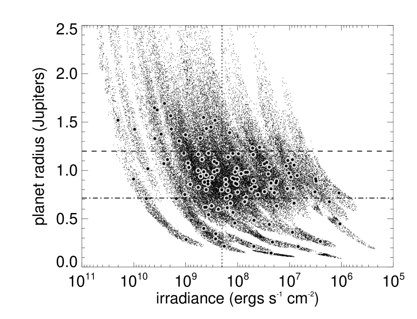
Figure 6: Radius vs. stellar irradiance of candidate giant planets (8$R_{\oplus}<R_{P}<22R_{\oplus}$) in the latest KOI release. These exclude the KOIs listed as false positives or “ambiguous” in the Table 1 of Demory & Seager (2011). Each large point represents values based on the stellar radius and luminosity of the Dartmouth stellar model that best reproduces the stellar parameters from the KIC. The dots represent 200 models chosen randomly from among all Dartmouth stellar models that cannot be ruled out at 95.4% ($2\sigma$) confidence. The vertical dotted line demarks the suggested boundary between high and low stellar irradiation regimes. Objects above the horizontal dashed line (1.2$R_{J}$) are considered “inflated”. Objects below the dot-dashed line ($8R_{\oplus}$) are smaller than reported in the KOI catalog and may have problematic Kepler lightcurve analyses. These were not included in the statistical analysis.

We simulated the impact of this systematic with an analysis of KOIs similar to, but not identical to that of D11. We selected all KOIs with estimated radii of $8R_{\oplus}<R_{p}<22R_{\oplus}$ from B12, excluding those listed as false positives or “ambiguous” in Table 1 of D11. As in Section 3.1, we identified the best-fit Dartmouth model for each host star based on a $\chi^{2}$ minimization of the difference with adjusted KIC values of $T_{e}$, $\log g$, and [Fe/H], after applying corrections of -100 K to $T_{e}$ and 0.17 dex to [Fe/H] (Br11). We assumed standard deviations of 200 K, 0.36 dex, and 0.3 dex, respectively based on Br11 and 190 stars where both KIC and spectroscopy-based parameters are available (B12). If no KIC value for [Fe/H] was available we assumed solar metallicity. To estimate the maximum possible effect, no constraints other than the Dartmouth evolutionary tracks were used, i.e. we equally weighted masses, ages between 1-13 Gyr, and metallicities between -2.5 and +0.5 dex. Orbit-averaged stellar irradition of the planet was calculated based on the model luminosity and mass, the orbital period, and assuming a circular orbit. (Non-circular orbits change the mean irradiance only slightly.) Planet radius was calculated from the transit depth and stellar model radius and we did not account for limb darkening. The encircled points in Figure 6 indicate the best-fit planet radius vs. irradiance. Three KOIs (217.01, 774.01, and 1547.01) have estimated irradiances $<2\times 10^{8}$ ergs s^-1 cm^-2 and $R_{p}>1.2R_{J}$, but only marginally so.

Fifteen KOIs have re-estimated radii $<0.5R_{J}$ even though the values listed in B12 exceed the criterion $>0.714R_{J}$. Twelve of these have KIC impact parameters $b>1$, suggesting problematic (or extreme grazing) transit solutions. Another (KOI 1419.01) has an implausible $b=0.994$ which is inconsistent with its transit duration of $t=1.36$ h and period $P=1.36$ d. KOI 377.02 (Kepler 9-b) has an erroneous transit depth reported in the MAST. The best-fit Dartmouth model assigns a somewhat smaller radius ($0.48R_{\odot}$) to the host star of KOI 1193.01 and thus makes the planet smaller as well. We excluded all planets with newly estimated radii $R_{p}<8R_{\oplus}$ from our analysis.

We assessed the trends produced by correlated errors in planet radius and irradiation by considering all Dartmouth models that satisfy $\chi^{2}<\chi_{min}^{2}+8.02$, where $\chi_{min}^{2}$ is the minimum (best-fit) value, and 8.02 is the $\Delta\chi^{2}$ corresponding to a 95.4% (2$\sigma$) confidence interval for $\nu=3$ degrees of freedom (stellar parameters). Because there are too many models to plot, we only show a random subsample of 200 such models for each KOI as the small points in Figure 6. These clearly show that correlated errors will tend to scatter points between the high irradiation/inflated and the low irradiation/uninflated regions of the diagram.

The paucity of KOIs with inflated radii ($R_{p}>1.2R_{J}$) in the low irradiance region (upper right hand domain of Figure 6) supports the contention that the inflation of giant planets is related to stellar irradiation or planet equilibrium temperature. Furthermore, Kendall’s and Spearman’s rank correlation tests of all KOIs with $R_{p}>0.714R_{J}$ yield $\tau$ values of 0.246 and 0.364, respectively, and corresponding $p$ (significance) values of $4.6\times 10^{-5}$ and $3.1\times 10^{-5}$. These low false-positive probabilities indicate a significant correlation between irradiation and plane radius. However, these statistics do not account for the systematic effect of correlated errors in radius and irradiation.

We simulated the effect of correlated errors by analyzing 10000 null realizations of the data where radii and orbital periods of KOIs were randomly shuffled among host stars and the transit depths were recomputed using Equation 1, thus destroying any intrinsic correlation between radius and irradiation. In computing each realization we include all KOIs with $R_{p}>3R_{\oplus}$ to account for small planets that may appear larger, but in each Monte Carlo realization, as with the real sample, we limited the statistical analysis to 8-22$R_{\oplus}$. New (“observed”) estimates of KIC stellar parameters were constructed from the “true” values by adding random, gaussian-distributed offsets with standard deviations of 200 K for $T_{e}$, 0.36 dex for $\log g$, and 0.3 dex for [Fe/H]. Best-fit Dartmouth models were found for each parameter set, the planet radii and irradiation values were determined, and the correlation statistics were calculated. New $p$ values for the fraction of KOIs in the low-irradiance/inflated-radius zone, and Kendall’s $\tau$, and Spearman’s $\tau$ were computed as the fraction of MC realizations that are smaller (more significant) than the observed values. The distributions for the first two metrics are shown in Figs. 7 and 8 and the $p$ values are $1.4\times 10^{-3}$ and $6\times 10^{-4}$, respectively. The result for the Spearman’s rank coefficient is similar, with $p=6\times 10^{-4}$.

3.6 Stellar metallicity and “shrunken” Jupiters

Dodson-Robinson (2012, hereafter DR12) reported a weakly significant ($p=0.02$ or $2.3\sigma$) trend of decreasing radius of Kepler (candidate) giant planet with increasing metallicity of the host star. She examined the ratio $R_{p}/R_{*}$ of 218 KOIs from Borucki et al. (2011) with estimated radii of 5-20 $R_{\oplus}$ and the correlation with estimated values of [Fe/H] from the KIC. She interpreted the decline as evidence that giant planets around metal-rich stars have larger solid cores and, for the same total planet mass, smaller radii (Guillot, 2005).

Figure 9 is an updated version of Figure 1 in DR12 based on the more recent release of KOIs with revised radii (Batalha, 2012). It includes 225 KOIs with $5R_{\oplus}<R_{p}<20R_{\oplus}$ and host stars with KIC-determined metallicities. As in Figure 1 from DR12, a running median ($N=21$) is plotted. The Kendall $\tau$ correlation coefficient is -0.032, indicating no signficant correlation ($p=0.48$). We were unable to reproduce the result of DR12 by simple cuts on this sample to approximate the earlier KOI sample, perhaps because many stellar radii (and hence planet radii) have been revised (Batalha, 2012). We also emphasize that the values of [Fe/H] in the KIC are no more accurate than $\pm$0.3 dex (Br11).

Irrespective of any physical phenomenon, one would expect to observe a decrease in $R_{p}/R_{*}$ with increasing metallicity simply because metal-rich dwarfs tend to be larger than metal-poor dwarfs, and hence transit depths will be smaller (Equation 1). We modeled this effect with 10000 Monte Carlo realizations of the KOI catalog. There are two effects from increasing the radii of the host stars of a given planet population: one is that transit depths will become smaller and the planets will appear to be smaller. The other is that some planets may fall below the lower radius cutoff (5$R_{\oplus}$) and be excluded from the analysis. The reverse is true for lower metallicity; planets appear larger and a few planets may exceed the maximum cutoff (20$R_{\oplus}$). We therefore considered KOIs over a broader (3-25$R_{\oplus}$) range of radii, adopted this sample as representing the intrinsic (“true”) distribution of radii, estimated their apparent radii from the radius of the star and transit depth, and then applied the same radius criteria as DR12. We randomly shuffled the planet population among the host stars, thus destroying any intrinsic radius-metallicity correlation, computed the radii of the stars using the Dartmouth stellar evolution models, and re-calculated the transit depths.

Each Monte Carlo host star was assigned the corrected $T_{e}$ of the actual star it replaced. We assigned an observed metallicity based on the KIC value, a systematic correction $\Delta$ of 0.17 dex (Br11), a random normally-distributed error $\sigma$ of 0.3 dex, and a prior distribution of intrinsic metallicities that is a guassian with mean $\bar{F}$ and standard deviation $\epsilon$. This is equivalent to drawing metallicities from a single normal distribution with mean $(\epsilon^{2}(\bar{F}+\Delta)+\sigma^{2}\bar{F})/(\epsilon^{2}+\sigma^{2})$ and standard deviation $\epsilon^{2}\sigma^{2}/(\epsilon^{2}+\sigma^{2})$. The radius of each Monte Carlo star was taken to be the median of all model radii with $\log g>4$ (presuming they are dwarf stars), [Fe/H] within 0.15 dex of the Monte Carlo model, and $T_{e}$ within 100 K. We did not apply any age criterion other than 1-13 Gyr. We then calculated $R_{p}/R_{*}$ using the shuffled planet radius and the median model radius stellar radius. For each Monte Carlo sample, we calculated Kendall’s $\tau$ and false positive probability for a correlation between the observed metallicities and the artificial transit depths.

Median-filtered ($n=21$) curves from these Monte Carlo realizations typically show a decline of $R_{p}/R_{*}$ with increasing metallicity. Figure 10 shows the distribution of $\tau$ from 10000 null realizations. The value of $\tau$ from the actual KOI sample is plotted as the dashed line. 61.6% of these null realizations produce a significant ($p<0.01$) correlation and 71.6% of values are below (and thus more significant than) the actual value of -0.032. For comparison the DR12 value is -0.17. Thus, negative correlations between metallicity and $R_{p}/R_{*}$ are to be expected soley as a consequence of the metallicity-radius relation of stars, although these Monte Carlo simulations indicate that there is a $\sim$40% chance that random errors in KIC [Fe/H] values would prevent such a correlation from being detected.

4 Discussion

We have shown that selection effects for both transiting planets, and the target stars of transit surveys, combined with uncertainties in stellar radii, can bias the properties of host stars and their planets. These effects are in addition to those previously identified by Gaudi (2005), Gaudi et al. (2005), and Pont et al. (2006), which concern effects arising from the sensitivity of detection efficiency to planet radius and period. We have analyzed the effects of these systematics on the Kepler survey and its catalogs of target stars and candidate planets, using current models of stellar evolution and galactic stellar populations to infer the properties of Kepler stars. We did not apply constraints from the relation between stellar density, transit duration, and orbital period because the relation also depends on unknown orbital eccentricity and argument of periastron, and is not applicable to non-KOI stars.

We found that Eddington bias from the steep distribution of KOIs with radius results in an overestimation of the overall frequency of planets with $R_{p}>2R_{\oplus}$ by about 15-20% of the actual value. We also find that Eddington bias acts to soften the “bump” in the distribution at Jupiter-size planets. This leads us to predict that the intrinsic peak at that radius is more pronounced. The effect on the distribution of smaller planets depends on whether the turnover in the radius distribution below 2$R_{\oplus}$ is real, or the result of incompleteness. If the former, Eddington bias acts to flatten the apparent slope of the radius distribution, and in this case we predict that the actual slope is steeper than the $\alpha=2.6$ power-law. Otherwise, the effect of Eddington bias on the power-law index is about 0.1.

We made statistical estimates of Malmquist bias as a consequence of the magnitude limit of the target catalog. The estimated bias for two-thirds of KOI systems, including most KOIs smaller than Neptune, is $<10$%. However, we found that bias is more prevalent and pronounced (up to a factor of two in radius) among larger candidate planets and their host stars, resulting from detection of these systems being governed by the apparent magnitude limit of the target catalog, rather than the SNR of transit detection. A Malmquist bias towards more luminous stars raises the possibility of inclusion of unidentified evolved stars within the Kepler target catalog (in addition to a number of deliberately selected and clearly identified giant stars). Nominally, stars with large radii were removed by a vetting process that used a criterion of Kepler detection of a $2R_{\oplus}$ planet (Batalha et al., 2010). However, KIC-derived stellar radii are based on estimates of log $g$ and many of these are problematic. KIC photometry provides no information for the gravity of stars with $T_{e}>5400$K ($g-r<0.65$), and subgiants would be assigned erroneously high log $g$ (Br11).

There are bona fida subgiants hosting KOIs, e.g. the F5 subgiant HD 179070 (Howell et al., 2012). Spectroscopy of stars hosting candidate giant planets has revealed other instances in which subgiants were misclassified as cooler, main sequence dwarfs in the KIC. Santerne et al. (2011) report a hot-Jupiter-hosting F-type subgiant ($M_{*}\approx 1.48M_{\odot}$, $R_{*}\approx 2.13R_{\odot}$). Based on spectra, they estimate $\log g=4.1\pm 0.2$, which is in contrast to its KIC value of 4.55. Likewise, the host of KOI-423b, assigned $\log g=4.45$ in the KIC, is an F7IV subgiant with $\log g=4.1$ (Bouchy et al., 2011). Three of five undiluted eclipsing binaries identified by Santerne et al. (2012) as false positives among Kepler giant planet candidates have masses larger than 1 M_⊙, and one of these is definitely an evolved star. The mean difference between 190 pairs of KIC and spectroscopic values of $\log g$ reported in Batalha (2012) is only 0.02 dex (standard deviation of 0.36 dex). Nevertheless, astroseismically-derived $\log g$ values average 0.05-0.17 dex lower than KIC values and astroseismically-determined radii are up to 50% larger (Verner et al., 2011; Bruntt et al., 2012).

Among KOI-hosting stars whose radius has been underestimated, small planets may actually be larger, even Jupiter-size planets. In turn, giant “planets” may turn out to be diluted or undiluted stellar companions, a significant source of astrophysical false positives in transit surveys (Charbonneau et al., 2004; Almenara et al., 2009). Based on a preliminary Doppler survey, Santerne et al. (2012) estimated that about 40% of candidate giant planets are false positives and about one quarter of those are undiluted eclipsing binaries. This also means that estimates of the occurrence of Jupiters on close-in orbits (Howard et al., 2012) must be revised downwards. Wright et al. (2012) report that the occurrence of “hot Jupiters” ($P<10$ d) in the Kepler catalog is only half that seen in Doppler surveys, and adjustment for a high false-positive rate would worsen this discrepancy.

One explanation for the discrepancy between the Kepler and Doppler surveys might be the presence of misidentified subgiant stars in the Kepler target catalog. The intrinsic distribution of planets may be different around evolved stars compared to main sequence stars. Planets have been discovered around subgiant stars (Butler et al., 2006), but giant planets appear to be rare with 0.6 AU ($P<120$ d) of clump GK giants (Sato et al., 2008, 2010; Johnson et al., 2011) - CoRoT-21b may be an exception (Patzold et al., 2011). The timescale of the decay of a planet’s orbit due to dissipation of tides in a star’s convective envelope scales as $R_{*}^{-8}M_{env}$, where $M_{env}$ is the mass of the envelope. Hot Jupiters are likely to be destroyed by infall and disruption inside the Roche lobe as a star evolves off the main sequence, expands, and its convective envelopes thicken (Kunitomo et al., 2011). Thus, one explanation for the comparative paucity of hot Jupiters in the KOI catalog is that, because of Malmquist bias, many Kepler targets are older stars or subgiants for which hot Jupiters cannot be detected, have been miscategorized as Neptunes, or have been destroyed by orbital decay. A comparison between the distributions of $\log g$ predicted by TRILEGAL and that of the KIC suggest no large ($>$10%) population of unidentified subgiants, however spectroscopy of candidate subgiants is needed to actually test this conjecture.

We have shown that, because metal-poor stars tend to have smaller radii than their metal-rich counterparts, stars with transiting planets will be biased towards metal-poor members, independent of any correlation between planets and metallicity. However, we estimate that this metallicity bias is only about -0.02 dex and can be neglected. Thus a comparison between the mean metallicity of stars with transiting planets and that of the overall target population is appropriate. The mean metallicity of M dwarfs with KOIs, -0.09 (Muirhead et al., 2012), and solar-type stars with small planets, -0.01 (Buchhave et al., 2012), appears similar to that of the solar neighborhood: Schlaufman & Laughlin (2010) report a mean metallicity of $-0.14\pm 0.06$ for a volume-limited local sample of M dwarfs using a photometric calibration, and Casagrande et al. (2011) report a median metallicity of -0.06 for all stars in the solar neighborhood. Whether the overall Kepler target population has a similar metallicity distribution is not yet known and additional observations are required. From our calculations we conclude that such a comparison would not suffer from significant metallicity bias, but must take into account a dilution factor because stars without transiting planets are not necessarily stars without planets. This dilution factor is large for a high planet occurrence (Mann et al., 2012).

We have shown how uncertainties in stellar radius or distance produce correlated errors in a planet’s radius and the radiation received from the host star. This effect can produce an artificial correlation in populations of planets where none exists. Recently, such a correlation has been found in both ground-based transit surveys and the Kepler catalog, and highlighted as a test of mechanisms to explain the “inflation” of giant planets on close-in orbits. We quantified the systematic effect of correlated errors in stellar radius in the case of the Kepler KOIs and show that, despite this systematic, the result of D11, i.e. that inflated planets are absent at low irradiance, is still significant. To maximize any systematic effect, we used a very broad range of metallicities (-2.5 to +0.5) and no constraint on stellar distance (e.g., from a model of galactic structure), thus further strengthening our conclusion.

Finally, we have shown how searches for trends of transiting planet radius with stellar properties may engender systematic errors unless the effect of those properties on apparent stellar radius - and hence planet radius - is taken into account. We examined the tentative (2.3$\sigma$) claim of DR12 that giant planets around metal-rich stars tend to have smaller transit depths, because they are smaller and perhaps have larger rocky cores. Performing a similar analysis on the most recent KOI catalog, we were unable to reproduce that trend. Moreover, we performed simulations that show that the trend observed by DR12 could be easily explained by the dependence of stellar radius on metallicity.

Two limitations of our analysis are that (i) we have asssumed gaussian-distributed errors in the corrected KIC parameters $T_{e}$, $\log g$, and [Fe/H], and (ii) that the construction of Bayesian priors on mass, age, and metallicity treat them as independent variables. Neither of these is absolutely correct; the first assumption probably produces an underestimate of the uncertainty in stellar radius while the second assumption produces an overestimate of the uncertainty. Of course, any inadequacies in the Dartmouth stellar evolution models themselves are not accounted for.

There are other systematics effects which may be present in transit surveys. Two-thirds of solar-type (F6-K3) stars are found in multiple systems (Raghavan et al., 2010). At the typical distance of Kepler KOIs with solar-type hosts (950 pc), one 4 arc-second pix subtends about 3800 AU, sufficient to include nearly all companions to primaries (Lépine et al., 2007; Raghavan et al., 2010). The presence of an unresolved companion, or any background star, will dilute the transit signal. Transits otherwise just above the detection threshold might be rendered invisible. As a consequence, members of multiple systems may be underrepresented among stars with transiting planets. For equal-mass binaries (twins) where the transit signal is lower by a factor of 2, the fractional noise will decrease by $\sqrt{2}$ (due to the doubling of the signal compared to a comparable single star) and thus the radius of the smallest detectable planet will increase by a factor of $2^{1/4}$, or about 1.2. For a power-law size distribution (Equation 3), the number of detectable planets per star will decrease by a factor of $2^{-\alpha/4}$, or 0.64 for $\alpha=2.6$. However, nearly-equal mass binaries represent only 12% of all binaries (Raghavan et al., 2010) and systems with mass ratios $<1$ and luminosity ratios $\ll 1$, where the dilution will be much smaller, are the norm. Star counts reach $\sim$1000 mag^-1 deg^-2 at $K_{p}=16$, and so there is only a few % chance of significant dilution by an unrelated star. To the extent that stellar variability inhibits transit detection, younger, and more active stars will be also underrepresented among KOIs.

The best defense against the systematic errors we have described is better characterization of the target stars of transit surveys, especially those hosting planets. This will reduce, but not entirely eliminate, these biases. Spectroscopic characterization and refinement of the properties of a fully representative sample of Kepler target stars, not just the KOI hosts, is vital to robust statistical analyses of the properties of transiting planets and their parent stars stars, and such programs are underway (Mann et al., 2012; Buchhave et al., 2012). Spectra of modest resolution ($R<1000$) (Malyuto et al., 2001) or SNR ($\sim 10$) (Katz et al., 1998) (but not both) can provide substantial improvements over photometry alone. The Gaia (originally Global Astrometric Interferometer for Astrophysics) mission, scheduled for launch in August 2013, will obtain parallaxes of stars as faint as 16th magnitude with a standard error of $\leq$40 $\mu$as (de Bruijne, 2012). This will allow the luminosity of a solar-type star to be determined with an error about 15% and its radius with an error of about 8%. The distance to brighter stars will be measured with even greater precision. Gaia will also obtain moderate-resolution spectra in a narrow region centered on the Ca II triplet region which can be used to classify stars (Kordopatis et al., 2011) and measure their radial velocities to a precision of a few km sec^-1. Radial velocites, combined with parallaxes, yield space motions and membership in distinct stellar populations (e.g. thin disk, halo). Gaia data will also benefit future transit surveys that will cover all of or a large part of the sky (Deming et al., 2009).

Figure 1: Uncertainty in radius of stars hosting KOIs, defined as one half of the range encompassing 68% of the probability distribution of radii. A few stars with the largest uncertainy are off-scale. As defined, the uncertainty can exceed the mean or most likely value and does in some cases. The adjusted KIC effective temperature is plotted on the abscissa. Solid points have KIC $\log g>4$ (“dwarfs”), while open points have $\log g<4$ (“giants”). While K-type dwarfs have uncertainties of as little as $\sim$15%, the radius of F- and many G-type stars is uncertain by $\geq 100$% because of the proximity of the giant and dwarf branches. The discontinuity at $T_{e}\sim 3900$ K is an artifact of the grid of models and the sensitivity to very large M giants.

Figure 2: Observed (uncorrected) distribution of KOI radii (open points and dashed line), and a distribution simulating the effects of Eddington bias (filled points and solid line). The latter is constructed by adjusting the ratio of each planet candidate by the ratio of the most likely stellar radius to every possible radius among stellar models, weighted by a likelihood factor (Equation 19). The two normalized distributions are equal at $R_{p}=3.4R_{\oplus}$. The biased distribution has a shallower slope at small radii, a less pronounced bump at Jupiter-size, and a higher occurrence of planets larger than the completeness limit.

Figure 3: Predicted biases in planet occurrence and power-law slope $\alpha$ due to Eddington bias for artifical planets with a power-law radius distribution placed around Kepler KOI-hosting stars. Howard et al. (2012) report that $\alpha\approx 2.6$ for planets with periods $P<50$ d. The slope of the scale-free power law distribution is only slightly affected by Eddington bias, but the apparent occurrence is biased upwards because more numerous smaller planets appear as larger planets due to errors in stellar radius.

Figure 4: Effect of Malmquist bias on the radii of stars and their planets. The ratio of the apparent or “naive” radius to the actual or “bias-informed” radius of 2061 KOIs is plotted vs. the nominal planet radius from the catalog of Batalha (2012). (239 others are around stars with incomplete parameters from the Kepler Input Catalog). The “naive” radius is the mean radius of possible stellar models weighted according to their consistency with KIC parameters and priors of mass, age, and metallicity. The “bias-informed” radius is the mean calculated using the scaling laws for Malmquist bias derived in Section 2.2. 1254 KOIs, and the vast majority of planet candidates smaller than Neptune, have predicted bias $<$10%, but many giant “planets” may have radii twice the nominal value and some may be astrophysical false positives, i.e. eclipsing stars.

Figure 5: Predicted bias in metalllicity in transiting planet-selected stars as a consequence of the relationships between transit depth, stellar radius, and stellar metallicity. The bias was calculated for all Quarter 6 Kepler target stars (regardless of whether or not they host KOIs) using Eqns. 2 and 11 and the methods described in Section 3.1. The upper locus of positive values are evolved stars, for which radius decreases with increasing metallicity.

Figure 7: Fraction of “inflated” ($R_{p}>1.2R_{J}$) candidate planets in the low irradiance ($<$2$\times 10^{8}$ ergs sec^-1 cm^-2) regime in 1000 Monte Carlo simulations of the KOI data set where planets were randomly shuffled among stars and stellar parameters were resampled according to standard errors in the KIC values. All KOIs with $R_{p}>3R_{\oplus}$ were used to generate the artificial planet populations, but only planets with $R_{p}>8R_{\oplus}$ were used in the analysis. The vertical dashed line marks the actual number (3). The $p$ value based on this distribution is $1.4\times 10^{-3}$.

Figure 8: Distribution of 1000 Kendall $\tau$ values for the correlation between planet radius and stellar irradiance using the same Monte Carlo realiziations of the giant planet KOIs as in Figure 7. The vertical dashed line marks the actual value ($\tau=0.31$), corresponding to a significane ($p$ value) of $6\times 10^{-4}$.

Figure 9: Ratio of planet radius to star radius of 225 Kepler candidate planets with estimated radii between 5 and 20 $R_{p}$ vs. metallicity estimates from the Kepler Input Catalog metallicities, uncertain by 0.3 dex (Br11). The curve is a running median (n=21). No trend with metallicity is apparent.

Figure 10: Distribution of Kendall $\tau$ values among 10000 Monte Carlo simulations of the KOI data set shown in Figure 9. Host star metallicities and KOI radii are scrambled, removing any intrinsic correlation between metallicity and planet radii. The only correlation here is due to the increasing radius of stars with metallicity. The dotted line is the value from the actual data. $3\sigma$ significance correspond to $\tau\approx-0.13$. Therefore, there is no significant correlation in the real data, and, because of the dependence of stellar radius on metallicity, a null sample would contain a significant ($p<0.01$) correlation about 60% of the time.

Table 1: Parameter values for TRILEGAL 1.5

Parameter	Value
Dust:
Extinction at $\infty$	0.0378
Scale height	110 pc
Scale length	100 kpc
Position of Sun:
Galactocentric radius	8700 pc
Height above disk	24.2 pc
Thin disk:
Zero-age scale height	95 pc
Radial length scale	2.8 kpc
Local surface density	59 M⊙ pc-2
Star formation rate	2-step
Thick disk:
Scale height	800 pc
Radial length scale	2.8 kpc
Local density	$1.5\times 10^{-3}$ M⊙ pc-2
Star formation rate	11-12 Gyr constant
Halo:
Shape	$r^{1/4}$ spheroid
Scale length	2.8 kpc
Oblateness	0.65
Local density	$1.5\times 10^{-4}$ M⊙ pc-2
Star formation rate	12-13 Gyr

References

- Agol et al. (2005) Agol, E., Steffen, J. H., Sari, R., & Clarkson, W. 2005, Mon. Not. Royal Astron. Soc., 359, 567
- Almenara et al. (2009) Almenara, J. M., et al. 2009, Astron. Astrophys., 506, 337
- Baraffe et al. (2003) Baraffe, I., Chabrier, G., Barman, T. S., Allard, F., & Hauschildt, P. H. 2003, Astron. Astrophys., 712, 701
- Batalha (2012) Batalha, N. M. 2012, arXiv:1202.5852
- Batalha et al. (2010) Batalha, N. M., et al. 2010, Astrophys. J., 713, L109
- Batygin & Stevenson (2010) Batygin, K., & Stevenson, D. J. 2010, Astrophys. J., 714, L238
- Bean et al. (2010) Bean, J. L., Seifahrt, A., Hartman, H., Nilsson, H., Wiedemann, G., Reiners, A., Dreizler, S., & Henry, T. J. 2010, Astrophys. J., 713, 410
- Bodenheimer et al. (2001) Bodenheimer, P., Lin, D. N. C., & Mardling, R. A. 2001, Astrophys. J., 548, 466
- Borucki et al. (2011) Borucki, W. J., et al. 2011, Astrophys. J., 736, article id. 19
- Bouchy et al. (2011) Bouchy, F., et al. 2011, Astron. Astrophys., 533, 83
- Boyajian et al. (2012) Boyajian, T. S., et al. 2012, Astrophys. J., 757, 112
- Brown et al. (2011) Brown, T. M., Latham, D. W. D., Everett, M. E. M., & Esquerdo, G. G. a. 2011, Astron. J., 142, 112
- Bruntt et al. (2012) Bruntt, H., et al. 2012, Mon. Not. Royal Astron. Soc., 423, 122
- Buchhave et al. (2012) Buchhave, L. a., et al. 2012, Nature, 486, 375
- Burrows et al. (2000) Burrows, A., Guillot, T., Hubbard, W., Marley, M. S., Saumon, D., Lunine, J. I., & Sudarsky, D. 2000, Astrophys. J., 534, L97
- Butler et al. (2006) Butler, R. P., Johnson, J. A., Marcy, G. W., Wright, J. T., Vogt, S. S., & Fischer, D. A. 2006, Publ. Astron. Soc. Pac., 118, 1685
- Casagrande et al. (2011) Casagrande, L., Schoenrich, R., Asplund, M., Cassisi, S., Ramirez, I., Melendez, J., Bensby, T., & Feltzing, S. 2011, Astron. Astrophys., 530, A138
- Charbonneau & Brown (2000) Charbonneau, D., & Brown, T. 2000, Astrophys. J., 529, L45
- Charbonneau et al. (2004) Charbonneau, D., Brown, T. M., Dunham, E. W., Latham, D. W., Looper, D. L., & Mandushev, G. 2004, in The Search for Other Worlds: 14th Astrophysics Conference, Vol. 713 (Melville, NY: AIP), 151–160
- Charbonneau et al. (2002) Charbonneau, D., Brown, T. M., Noyes, R. W., & Gilliland, R. L. 2002, Astrophys. J., 568, 374
- Charbonneau & Deming (2007) Charbonneau, D., & Deming, D. 2007, arXiv:0706.1047
- Charbonneau et al. (2005) Charbonneau, D., et al. 2005, Astrophys. J., 626, 523
- Cox (2000) Cox, A. N. 2000, Allen’s Astrophysical Quantities (New York: AIP Press, Springer)
- Cumming et al. (2008) Cumming, A., Butler, R., Marcy, G., & Vogt, S. 2008, Publ. Astron. Soc. Pac., 120, 531
- de Bruijne (2012) de Bruijne, J. H. J. 2012, Astrophys. Space Sci., online fir
- Deming et al. (2009) Deming, D., et al. 2009, Publ. Astron. Soc. Pac., 121, 952
- Demory & Seager (2011) Demory, B.-O., & Seager, S. 2011, Astrophys. J. Supp. Ser., 197, 12
- Désert et al. (2011) Désert, J.-M., Kempton, E. M.-R., Berta, Z. K., Charbonneau, D., Irwin, J., Fortney, J., Burke, C. J., & Nutzman, P. 2011, Astrophys. J., 731, L40
- Dodson-Robinson (2012) Dodson-Robinson, S. E. 2012, Astrophys. J., 752, 72
- Dotter et al. (2008) Dotter, A., Chaboyer, B., Jevremović, D., Kostov, V., Baron, E., & Ferguson, J. W. 2008, Astrophys. J., 178, 89
- Eddington (1913) Eddington, A. S. 1913, Mon. Not. Royal Astron. Soc., 73, 359
- Enoch et al. (2012) Enoch, B., Collier-Cameron, A., & Horne, K. 2012, Astron. Astrophys., 540, 99
- Fischer & Valenti (2005) Fischer, D. A., & Valenti, J. 2005, Astrophys. J., 622, 1102
- Ford et al. (2011) Ford, E. B., et al. 2011, Astrophys. J. Supp. Ser., 197, 2
- Fortney et al. (2010) Fortney, J. J., Baraffe, I., & Militzer, B. 2010, in Exoplanets (University of Arizon Press), 397
- Fressin et al. (2009) Fressin, F., Guillot, T., & Nesta, L. 2009, Astron. Astrophys., 504, 605
- Gaidos et al. (2012) Gaidos, E., Fischer, D. A., Mann, A. W., & Lépine, S. 2012, Astrophys. J., 746, 36
- Gaidos et al. (2007) Gaidos, E., Haghighipour, N., Agol, E., Latham, D., Raymond, S. N., & Rayner, J. 2007, Science, 318, 210
- Gaudi (2005) Gaudi, B. S. 2005, Astrophys. J., 628, L73
- Gaudi et al. (2005) Gaudi, B. S., Seager, S., & Mallen‐Ornelas, G. 2005, Astrophys. J., 623, 472
- Girardi et al. (2005) Girardi, L., Groenewegen, M., Hatziminaoglou, E., & Da Costa, L. 2005, Astron. Astrophys., 436, 895
- Gonzalez (1998) Gonzalez, G. 1998, Astron. Astrophys., 238, 221
- Grasset et al. (2009) Grasset, O., Schneider, J., & Sotin, C. 2009, Astrophys. J., 693, 722
- Guillot (2005) Guillot, T. 2005, Annu. Rev. Earth Planet. Sci., 33, 493
- Guillot et al. (1996) Guillot, T., Burrows, A., Hubbard, W., Lunine, J. I., & Saumon, D. 1996, Astrophys. J., 459, L35
- Henry et al. (2000) Henry, G. W., Marcy, G. W., Butler, R. P., & Vogt, S. S. 2000, Astrophysical Journal, 529, L41
- Howard et al. (2010) Howard, A. W., et al. 2010, Science, 330, 653
- Howard et al. (2012) —. 2012, Astrophys. J. Supp. Ser., 201, 15
- Howell et al. (2012) Howell, S. B., et al. 2012, Astrophys. J., 746, 123
- Huber et al. (2010) Huber, D., et al. 2010, Astrophys. J., 723, 1607
- Johnson et al. (2011) Johnson, J., Clanton, C., & Howard, A. 2011, Astrophys. J., 197, 26
- Johnson et al. (2010) Johnson, J. J., Aller, K. K., Howard, A. A., & Crepp, J. 2010, Publ. Astron. Soc. Pac., 122, 233
- Katz et al. (1998) Katz, D., Soubiran, C., Cayrel, R., Adda, M., & Cautain, R. 1998, Astron. Astrophys., 160, 151
- Knutson et al. (2008) Knutson, H. A., Charbonneau, D., Allen, L. E., Burrows, A., & Megeath, S. T. 2008, Astrophys. J., 673, 526
- Konacki et al. (2003) Konacki, M., Torres, G., Jha, S., & Sasselov, D. D. 2003, Nature, 421, 507
- Kordopatis et al. (2011) Kordopatis, G., Recio-Blanco, A., de Laverny, P., Bijaoui, A., Hill, V., Gilmore, G., Wyse, R. F. G., & Ordenovic, C. 2011, Astron. Astrophys., 535, A106
- Kroupa (2002) Kroupa, P. 2002, in Modes of Star Formation and the Origin of Field Populations. ASP Conference Series Vol. 285, ed. E. K. Grebel & W. Brandner (ASP)
- Kunitomo et al. (2011) Kunitomo, M., Ikoma, M., Sato, B., Katsuta, Y., & Ida, S. 2011, Astrophys. J., 737, 66
- Laughlin et al. (2011) Laughlin, G., Crismani, M., & Adams, F. C. 2011, Astrophys. J., 729, L7
- Lepine et al. (2012) Lepine, S., Hilton, E. J., Mann, A. W., Wilde, M., Rojas-Ayala, B., Cruz, K. L., & Gaidos, E. 2012, arXiv1206.5991L
- Lépine et al. (2007) Lépine, S., Rich, R. M., & Shara, M. M. 2007, Astrophys. J., 669, 1235
- Lissauer et al. (2012) Lissauer, J. J., et al. 2012, Astrophys. J., 750, 112
- Liu & Chaboyer (2000) Liu, W. M., & Chaboyer, B. 2000, Astrophys. J., 544, 818
- Malmquist (1922) Malmquist, K. G. 1922, Lund Medd. Ser. I
- Malyuto et al. (2001) Malyuto, V., Lazauskaite, R., & Shvelidze, T. 2001, New Astron., 6, 381
- Mann et al. (2012) Mann, A. W., Gaidos, E., Lepine, S., & Hilton, E. J. 2012, Astrophys. J., 753, 90
- Mayor et al. (2009) Mayor, M., et al. 2009, Astron. Astrophys., 493, 527
- Mayor et al. (2011) —. 2011, Astron. Astrophys., 507, 487
- Mizuno (1980) Mizuno, H. 1980, Prog. Theor. Phys., 64, 544
- Morton & Johnson (2011) Morton, T. T. D., & Johnson, J. A. J. 2011, Astrophys. J., 738, 170
- Muirhead et al. (2012) Muirhead, P., Hamren, K., Schlawin, E., Rojas-Ayala, B., Covey, K. R., & Lloyd, J. P. 2012, Astrophys. J., 750, L37
- Oswalt et al. (1996) Oswalt, T. D., Smith, J. A., Wood, M. A., & Hintzen, P. 1996, Nature, 382, 692
- Patzold et al. (2011) Patzold, M., Endl, M., Czismadia, S., Gandolfi, D., Jorda, L., Grziwa, S., Carone, L., & Pasternacki, T. 2011, in EPSC-DPS Joint Meeting, 1192
- Pinsonneault et al. (2012) Pinsonneault, M., An, D., Molenda-Żakowicz, J., Chaplan, W. J., Metcalfe, T. S., & Bruntt, H. 2012, Astrophys. J. Supp. Ser., 199, 30
- Pont et al. (2006) Pont, F., Zucker, S., & Queloz, D. 2006, Mon. Not. Royal Astron. Soc., 373, 231
- Raghavan et al. (2010) Raghavan, D., et al. 2010, Astrophys. J. Supp. Ser., 190, 1
- Rogers et al. (2011) Rogers, L., Bodenheimer, P., Lissauer, J., & Seager, S. 2011, Astrophys. J., 738, 59
- Rowe et al. (2008) Rowe, J. F., et al. 2008, Astrophys. J., 689, 1345
- Ruchti et al. (2011) Ruchti, G. R., et al. 2011, Astrophys. J., 737, 9
- Santerne et al. (2011) Santerne, A., Bouchy, F., Deleuil, M., Moutou, C., Eggenberger, A., Ehrenreich, D., Gry, C., & Udry, S. 2011, Astron. Astrophys., 528, A63
- Santerne et al. (2012) Santerne, A., Moutou, C., Bouchy, F., Bonomo, A. S., Deleuil, M., & Santos, N. C. 2012, Astron. Astrophys., 545, 76
- Santos et al. (2004) Santos, N. C., Israelian, G., & Mayor, M. 2004, Astronomy and Astrophysics, 415, 1153
- Sato et al. (2008) Sato, B., Toyota, E., Omiya, M., & Izumiura, H. 2008, Publ. Astron. Soc. Japan, 60, 1317
- Sato et al. (2010) Sato, B., et al. 2010, Publ. Astron. Soc. Japan, 62, 1063
- Schlaufman & Laughlin (2011) Schlaufman, K., & Laughlin, G. 2011, Astrophys. J., 738, 177
- Schlaufman & Laughlin (2010) Schlaufman, K. C., & Laughlin, G. 2010, Astron. Astrophys., 519, A105
- Schlegel et al. (1998) Schlegel, D., Finkbeiner, D., & Davis, M. 1998, The Astrophysical Journal, 500, 535
- Schneider et al. (2011) Schneider, J., Dedieu, C., Sidaner, P. L., Savalle, R., & Zolotukhin, I. 2011, Astronomy and Astrophysics, 532, A79
- Seager et al. (2007) Seager, S., Kuchner, M. J., Hier-Majumder, C., Militzer, B., & Hier‐Majumder, C. a. 2007, Astrophys. J., 669, 1279
- Showman (2002) Showman, A. 2002, Astron. Astrophys., 385, 166
- Sousa et al. (2008) Sousa, S. G., et al. 2008, Astron. Astrophys., 381, 373
- Tarter et al. (2007) Tarter, J. C., et al. 2007, Astrobiology, 7, 30
- Valencia et al. (2007) Valencia, D., Sasselov, D. D., & O’Connell, R. J. 2007, Astrophys. J., 665, 1413
- Vanhollebeke et al. (2009) Vanhollebeke, E., Groenewegen, M. a. T., & Girardi, L. 2009, Astron. Astrophys., 498, 95
- Verner et al. (2011) Verner, G. a., et al. 2011, The Astrophysical Journal, 738, L28
- Wolfgang & Laughlin (2012) Wolfgang, A., & Laughlin, G. 2012, Astrophys. J., 750, 148
- Woolf & West (2012) Woolf, V. M., & West, A. A. 2012, Mon. Not. Royal Astron. Soc., 422, 1489
- Wright et al. (2012) Wright, J., Marcy, G., Howard, A., Johnson, J. A., Morton, T., & Fischer, D. A. 2012, Astrophys. J., 753, 160
- Zielinski et al. (2012) Zielinski, P., Niedzielski, A., Wolszczan, A., Adamow, M., & Nowak, G. 2012, arXiv:1206.6276