Study of $X_{c}(3250)$ as a $D_{0}^{*}(2400)N$ molecular state

Abstract

We present a QCD sum rule analysis for the newly observed resonance $X_{c}(3250)$ by assuming it as a $D_{0}^{*}(2400)N$ molecular state. Technically, contributions of operators up to dimension $12$ are included in the operator product expansion (OPE). We find that it is difficult to find the conventional OPE convergence in this work. By trying releasing the rigid OPE convergence criterion, one could find that the OPE convergence is still under control in the present work and the numerical result for $D_{0}^{*}(2400)N$ state is $3.18\pm 0.51~{}\mbox{GeV}$, which is in agreement with the experimental data of $X_{c}(3250)$. In view of that the conventional OPE convergence is not obtained here, thus only weak conclusions can be drawn regarding the explanation of $X_{c}(3250)$ in terms of a $D_{0}^{*}(2400)N$ molecular state. As a byproduct, the mass for the bottom counterpart $\bar{B}_{0}^{*}N$ state is predicted to be $6.50\pm 0.49~{}\mbox{GeV}$.

I Introduction

Very recently, BaBar Collaboration reported the measurement of the baryonic $B$ decay $B^{-}\rightarrow\Sigma_{c}^{++}\bar{p}\pi^{-}\pi^{-}$ and observed a new structure in the $\Sigma_{c}^{++}\pi^{-}\pi^{-}$ invariant mass spectrum at $3.25~{}\mbox{GeV}$ X . For simplicity, one could name the new structure as $X_{c}(3250)$. Soon after the experimental observation, He et al. have suggested that $X_{c}(3250)$ could be a $D_{0}^{*}(2400)N$ molecular state from an effective Lagrangian calculation X-th . Theoretically, the molecular concept is well and truly not a new topic but with a history. It was put forward nearly 40 years ago in Ref. Voloshin and was predicted that molecular states have a rich spectroscopy in Ref. Glashow . The possible deuteron-like two-meson bound states were studied in Ref. NAT . In recent years, some of “X”, “Y”, and “Z” new hadrons are ranked as possible molecular candidates. Such as, $X(3872)$ could be a $D\bar{D}^{*}$ molecular state X3872 ; X3872-1 ; X3872-2 ; X3872-3 ; X3872-4 ; $X(4350)$ is interpreted as a $D_{s}^{*}\bar{D}_{s0}^{*}$ state X4350-Zhang ; X4350-Ma ; $Y(4260)$ is proposed to be a $\chi_{c}\rho^{0}$ Y4260-Liu or an $\omega\chi_{c1}$ state Y4260-Yuan ; $Z^{+}(4430)$ is deciphered as a $D^{*}\bar{D}_{1}$ state theory-Z4430n ; theory-Z4430 ; $Z_{b}(10610)$ and $Z_{b}(10650)$ could be $B^{*}\bar{B}$ and $B^{*}\bar{B}^{*}$ states, respectively Zb ; Zb1 . Especially, there already have a lot of works discussing baryon resonances with meson-baryon molecular structures, e.g. new . If molecular states can be completely confirmed by experiment, QCD will be further testified and then one will understand the QCD low-energy behaviors more deeply. Therefore, it is interesting to study whether the newly observed $X_{c}(3250)$ state could be a $D_{0}^{*}(2400)N$ molecular state.

In the real world, quarks are confined inside hadrons and the strong interaction dynamics of hadronic systems is governed by nonperturbative QCD effect completely. Many questions concerning dynamics of the quarks and gluons at large distances remain unanswered or understood only at a qualitative level. It is quite difficult to extract hadronic information quantitatively from the basic theory of QCD. The QCD sum rule method svzsum is a nonperturbative formulation firmly based on the first principle of QCD, which has been successfully applied to conventional hadronic systems, i.e. mesons or baryons (for reviews see overview1 ; overview2 ; overview3 ; overview4 and references therein). For multiquark states, there have appeared fruitful results from QCD sum rules these years (for a review on multiquark QCD sum rules one can see XYZ and references therein). In particular for hadrons containing five quarks, some authors began to study light pentaquark states in Refs. pentaquark . The application of QCD sum rules to heavy pentaquark states was performed in Ref. pentaquark-heavy for the first time.

In this work, we devote to investigating that whether the newly observed resonance $X_{c}(3250)$ could be a $D_{0}^{*}(2400)N$ molecular state ($D_{0}^{*}$ has a quark content $c\bar{q}$) in the framework of QCD sum rules. As a byproduct, the mass for its bottom counterpart $\bar{B}_{0}^{*}N$ is also predicted on the assumption that it could exist ($\bar{B}_{0}^{*}$ has a quark content $b\bar{q}$ and one should note that it has not been observed). In theory, one could expect that the $\bar{B}_{0}^{*}$ meson should be assigned the same spin parity $0^{+}$ as $D_{0}^{*}$. The rest of the paper is organized as three sections. We discuss QCD sum rules for molecular states in Sec. II utilizing similar techniques as our previous works Zhang . The numerical analysis and discussions are presented in Sec. III, and masses of $D_{0}^{*}(2400)N$ and $\bar{B}_{0}^{*}N$ molecular states are extracted out. The Sec. IV includes a brief summary and outlook.

II QCD sum rules for molecular states

The QCD sum rules for molecular states are constructed from the two-point correlation function

$$\Pi(q^{2})=i\int d^{4}x\mbox{e}^{iq.x}\langle 0|T[j(x)\overline{j}(0)]|0\rangle.$$ (1)

In full theory, the interpolating current for $D_{0}^{*}(2400)$ or $\bar{B}_{0}^{*}$ meson can be found in Ref. reinders , and the one for nucleon $N$ has been listed in Ref. baryon-current . One can construct the $D_{0}^{*}(2400)N$ or $\bar{B}_{0}^{*}N$ molecular state current from meson-baryon type of fields

$$j = (\bar{q}^{c^{{}^{\prime}}}Q^{c^{{}^{\prime}}})(\varepsilon_{abc}q_{1}^{Ta}C\gamma_{\mu}q_{2}^{b}\gamma_{5}\gamma^{\mu}q_{3}^{c}),$$ (2)

where $Q$ is heavy quark $c$ or $b$, and $q$, $q_{1}$, $q_{2}$, as well as $q_{3}$ denote light quarks. The index $T$ means matrix transposition, $C$ is the charge conjugation matrix, with $a$, $b$, $c$ and $c^{\prime}$ are color indices. One should note that meson-baryon molecules in the real world are long objects in which the meson and the baryon are far away from each other. The currents in this work and in most of the QCD sum rule works are local and the five field operators here act at the same space-time point. It is a limitation inherent in the QCD sum rule disposal of the hadrons since the bound states are not point particles in a rigorous manner.

Lorentz covariance implies that the two-point correlation function in Eq. (1) has the form

$$\Pi(q^{2})=\Pi_{1}(q^{2})+\hbox to0.0pt{/\hss}q\Pi_{2}(q^{2}).$$ (3)

According to the philosophy of QCD sum rules, the correlator is evaluated in two ways. Phenomenologically, the correlator can be expressed as a dispersion integral over a physical spectral function

$$\Pi(q^{2})=\lambda^{2}_{H}\frac{\hbox to0.0pt{/\hss}q+M_{H}}{M_{H}^{2}-q^{2}}+\frac{1}{\pi}\int_{s_{0}}^{\infty}ds\frac{\mbox{Im}\Pi_{1}^{\mbox{phen}}(s)+\hbox to0.0pt{/\hss}q\mbox{Im}\Pi_{2}^{\mbox{phen}}(s)}{s-q^{2}}+\mbox{subtractions},$$ (4)

where $M_{H}$ is the mass of the hadronic resonance, and $\lambda_{H}$ gives the coupling of the current to the hadron $\langle 0|j|H\rangle=\lambda_{H}u(p,s)$. In the OPE side, short-distance effects are taken care of by Wilson coefficients, while long-distance confinement effects are included as power corrections and parameterized in terms of vacuum expectation values of local operators, the so-called condensates. One can write the correlation function in the OPE side in terms of a dispersion relation

$$\Pi(q^{2})=\int_{m_{Q}^{2}}^{\infty}ds\frac{\rho_{1}(s)}{s-q^{2}}+\Pi_{1}^{\mbox{cond}}(q^{2})+\hbox to0.0pt{/\hss}q\bigg{\{}\int_{m_{Q}^{2}}^{\infty}ds\frac{\rho_{2}(s)}{s-q^{2}}+\Pi_{2}^{\mbox{cond}}(q^{2})\bigg{\}},$$ (5)

where the spectral density is given by the imaginary part of the correlation function

$$\rho_{i}(s)=\frac{1}{\pi}\mbox{Im}\Pi_{i}^{\mbox{OPE}}(s),~{}~{}i=1,2.$$ (6)

Technically, one works at leading order in $\alpha_{s}$ and considers condensates up to dimension $12$. To keep the heavy-quark mass finite, one can use the momentum-space expression for the heavy-quark propagator reinders

$$S_{Q}(p) = \frac{i}{\hbox to0.0pt{/\hss}p-m_{Q}}-\frac{i}{4}gt^{A}G^{A}_{\kappa\lambda}(0)\frac{1}{(p^{2}-m_{Q}^{2})^{2}}[\sigma_{\kappa\lambda}(\hbox to0.0pt{/\hss}p+m_{Q})+(\hbox to0.0pt{/\hss}p+m_{Q})\sigma_{\kappa\lambda}]$$

$${}-\frac{i}{4}g^{2}t^{A}t^{B}G^{A}_{\alpha\beta}(0)G^{B}_{\mu\nu}(0)\frac{\hbox to0.0pt{/\hss}p+m_{Q}}{(p^{2}-m_{Q}^{2})^{5}}[\gamma^{\alpha}(\hbox to0.0pt{/\hss}p+m_{Q})\gamma^{\beta}(\hbox to0.0pt{/\hss}p+m_{Q})\gamma^{\mu}(\hbox to0.0pt{/\hss}p+m_{Q})\gamma^{\nu}$$

$${}+\gamma^{\alpha}(\hbox to0.0pt{/\hss}p+m_{Q})\gamma^{\mu}(\hbox to0.0pt{/\hss}p+m_{Q})\gamma^{\beta}(\hbox to0.0pt{/\hss}p+m_{Q})\gamma^{\nu}+\gamma^{\alpha}(\hbox to0.0pt{/\hss}p+m_{Q})\gamma^{\mu}(\hbox to0.0pt{/\hss}p+m_{Q})\gamma^{\nu}(\hbox to0.0pt{/\hss}p+m_{Q})\gamma^{\beta}](\hbox to0.0pt{/\hss}p+m_{Q})$$

$${}+\frac{i}{48}g^{3}f^{ABC}G^{A}_{\gamma\delta}G^{B}_{\delta\varepsilon}G^{C}_{\varepsilon\gamma}\frac{1}{(p^{2}-m_{Q}^{2})^{6}}(\hbox to0.0pt{/\hss}p+m_{Q})[\hbox to0.0pt{/\hss}p(p^{2}-3m_{Q}^{2})+2m_{Q}(2p^{2}-m_{Q}^{2})](\hbox to0.0pt{/\hss}p+m_{Q}).$$

The light-quark part of the correlation function can be calculated in the coordinate space, with the light-quark propagator

$$S_{ab}(x) = \frac{i\delta_{ab}}{2\pi^{2}x^{4}}\hbox to0.0pt{/\hss}x-\frac{m_{q}\delta_{ab}}{4\pi^{2}x^{2}}-\frac{i}{32\pi^{2}x^{2}}t^{A}_{ab}gG^{A}_{\mu\nu}(\hbox to0.0pt{/\hss}x\sigma^{\mu\nu}+\sigma^{\mu\nu}\hbox to0.0pt{/\hss}x)-\frac{\delta_{ab}}{12}\langle\bar{q}q\rangle+\frac{i\delta_{ab}}{48}m_{q}\langle\bar{q}q\rangle\hbox to0.0pt{/\hss}x$$ (8)

$${}-\frac{x^{2}\delta_{ab}}{3\cdot 2^{6}}\langle g\bar{q}\sigma\cdot Gq\rangle+\frac{ix^{2}\delta_{ab}}{2^{7}\cdot 3^{2}}m_{q}\langle g\bar{q}\sigma\cdot Gq\rangle\hbox to0.0pt{/\hss}x-\frac{x^{4}\delta_{ab}}{2^{10}\cdot 3^{3}}\langle\bar{q}q\rangle\langle g^{2}G^{2}\rangle,$$

which is then Fourier-transformed to the momentum space in $D$ dimension. The resulting light-quark part is combined with the heavy-quark part before it is dimensionally regularized at $D=4$. Equating the two sides for $\Pi(q^{2})$ and assuming quark-hadron duality yield the sum rules, from which masses of hadrons can be determined. After making a Borel transform and transferring the continuum contribution to the OPE side, the sum rules can be written as

$$\lambda^{2}_{H}M_{H}e^{-M_{H}^{2}/M^{2}} = \int_{m_{Q}^{2}}^{s_{0}}ds\rho_{1}(s)e^{-s/M^{2}}+\hat{B}\Pi_{1}^{\mbox{cond}},$$ (9)

$$\lambda^{2}_{H}e^{-M_{H}^{2}/M^{2}} = \int_{m_{Q}^{2}}^{s_{0}}ds\rho_{2}(s)e^{-s/M^{2}}+\hat{B}\Pi_{2}^{\mbox{cond}},$$ (10)

where $M^{2}$ indicates the Borel parameter. To eliminate the hadron coupling constant $\lambda_{H}$ and extract the resonance mass $M_{H}$, one can take the derivative of Eq. (9) with respect to $1/M^{2}$, divide the result by itself and deal with Eq. (10) in the same way to get

$$M_{H}^{2} = \bigg{\{}\int_{m_{Q}^{2}}^{s_{0}}ds\rho_{1}(s)se^{-s/M^{2}}+d/d(-\frac{1}{M^{2}})\hat{B}\Pi_{1}^{\mbox{cond}}\bigg{\}}/\bigg{\{}\int_{m_{Q}^{2}}^{s_{0}}ds\rho_{1}(s)e^{-s/M^{2}}+\hat{B}\Pi_{1}^{\mbox{cond}}\bigg{\}},$$ (11)

$$M_{H}^{2} = \bigg{\{}\int_{m_{Q}^{2}}^{s_{0}}ds\rho_{2}(s)se^{-s/M^{2}}+d/d(-\frac{1}{M^{2}})\hat{B}\Pi_{2}^{\mbox{cond}}\bigg{\}}/\bigg{\{}\int_{m_{Q}^{2}}^{s_{0}}ds\rho_{2}(s)e^{-s/M^{2}}+\hat{B}\Pi_{2}^{\mbox{cond}}\bigg{\}},$$ (12)

where

$$\rho_{i}(s) = \rho_{i}^{\mbox{pert}}(s)+\rho_{i}^{\langle\bar{q}q\rangle}(s)+\rho_{i}^{\langle\bar{q}q\rangle^{2}}(s)+\rho_{i}^{\langle g\bar{q}\sigma\cdot Gq\rangle}(s)+\rho_{i}^{\langle g^{2}G^{2}\rangle}(s)+\rho_{i}^{\langle g^{3}G^{3}\rangle}(s)+\rho_{i}^{\langle\bar{q}q\rangle^{3}}(s)+\rho_{i}^{\langle\bar{q}q\rangle\langle g\bar{q}\sigma\cdot Gq\rangle}(s)$$ (13)

$$+\rho_{i}^{\langle g\bar{q}\sigma\cdot Gq\rangle\langle g\bar{q}\sigma\cdot Gq\rangle}(s)+\rho_{i}^{\langle\bar{q}q\rangle\langle g^{2}G^{2}\rangle}(s)+\rho_{i}^{\langle\bar{q}q\rangle\langle g^{3}G^{3}\rangle}(s)+\rho_{i}^{\langle g^{2}G^{2}\rangle\langle g\bar{q}\sigma\cdot Gq\rangle}(s),~{}~{}i=1,2.$$

As a matter of fact, many terms of $\rho_{1}(s)$ are approximate to zero because they are proportional to light quarks’ masses in the calculations. Thereby, we merely present the spectral densities resulted from $\Pi_{2}(q^{2})$ here. Concretely, they can be written as

$$\rho_{2}^{\mbox{pert}}(s) = \frac{1}{3\cdot 5^{2}\cdot 2^{16}\pi^{8}}\int_{\Lambda}^{1}d\alpha\frac{(1-\alpha)^{6}}{\alpha^{5}}(\alpha s-m_{Q}^{2})^{4}(\alpha s+4m_{Q}^{2}),$$

$$\rho_{2}^{\langle\bar{q}q\rangle}(s) = \frac{m_{Q}\langle\bar{q}q\rangle}{3\cdot 2^{11}\pi^{6}}\int_{\Lambda}^{1}d\alpha\frac{(1-\alpha)^{4}}{\alpha^{3}}(\alpha s-m_{Q}^{2})^{3},$$

$$\rho_{2}^{\langle\bar{q}q\rangle^{2}}(s) = \frac{\langle\bar{q}q\rangle^{2}}{3\cdot 2^{8}\pi^{4}}\int_{\Lambda}^{1}d\alpha\frac{(1-\alpha)^{3}}{\alpha^{2}}(\alpha s-m_{Q}^{2})(\alpha s+m_{Q}^{2}),$$

$$\rho_{2}^{\langle g\bar{q}\sigma\cdot Gq\rangle}(s) = -\frac{m_{Q}\langle g\bar{q}\sigma\cdot Gq\rangle}{2^{11}\pi^{6}}\int_{\Lambda}^{1}d\alpha\frac{(1-\alpha)^{3}}{\alpha^{2}}(\alpha s-m_{Q}^{2})^{2},$$

$$\rho_{2}^{\langle g^{2}G^{2}\rangle}(s) = \frac{m_{Q}^{2}\langle g^{2}G^{2}\rangle}{5\cdot 3^{2}\cdot 2^{16}\pi^{8}}\int_{\Lambda}^{1}d\alpha\frac{(1-\alpha)^{6}}{\alpha^{5}}(\alpha s-m_{Q}^{2})(\alpha s-2m_{Q}^{2}),$$

$$\rho_{2}^{\langle g^{3}G^{3}\rangle}(s) = \frac{\langle g^{3}G^{3}\rangle}{5\cdot 3^{2}\cdot 2^{18}\pi^{8}}\int_{\Lambda}^{1}d\alpha\frac{(1-\alpha)^{6}}{\alpha^{5}}[(\alpha s)^{2}-9\alpha sm_{Q}^{2}+10m_{Q}^{4}],$$

$$\rho_{2}^{\langle\bar{q}q\rangle^{3}}(s) = \frac{m_{Q}\langle\bar{q}q\rangle^{3}}{3\cdot 2^{4}\pi^{2}}\int_{\Lambda}^{1}d\alpha(1-\alpha),$$

$$\rho_{2}^{\langle\bar{q}q\rangle\langle g\bar{q}\sigma\cdot Gq\rangle}(s) = -\frac{\langle\bar{q}q\rangle\langle g\bar{q}\sigma\cdot Gq\rangle}{2^{8}\pi^{4}}s\int_{\Lambda}^{1}d\alpha(1-\alpha)^{2},$$

$$\rho_{2}^{\langle g\bar{q}\sigma\cdot Gq\rangle\langle g\bar{q}\sigma\cdot Gq\rangle}(s) = \frac{\langle g\bar{q}\sigma\cdot Gq\rangle^{2}}{2^{10}\pi^{4}}\int_{\Lambda}^{1}d\alpha(1-\alpha),$$

$$\rho_{2}^{\langle\bar{q}q\rangle\langle g^{2}G^{2}\rangle}(s) = \frac{m_{Q}\langle\bar{q}q\rangle\langle g^{2}G^{2}\rangle}{3^{2}\cdot 2^{13}\pi^{6}}\int_{\Lambda}^{1}d\alpha\frac{(1-\alpha)^{2}}{\alpha^{3}}[6\alpha^{2}(\alpha s-m_{Q}^{2})+(1-\alpha)^{2}(3\alpha s-4m_{Q}^{2})],$$

$$\rho_{2}^{\langle\bar{q}q\rangle\langle g^{3}G^{3}\rangle}(s) = -\frac{m_{Q}\langle\bar{q}q\rangle\langle g^{3}G^{3}\rangle}{3\cdot 2^{14}\pi^{6}}\int_{\Lambda}^{1}d\alpha\frac{(1-\alpha)^{4}}{\alpha^{3}},$$

$$\rho_{2}^{\langle g^{2}G^{2}\rangle\langle g\bar{q}\sigma\cdot Gq\rangle}(s) = -\frac{m_{Q}\langle g^{2}G^{2}\rangle\langle g\bar{q}\sigma\cdot Gq\rangle}{3\cdot 2^{13}\pi^{6}}\int_{\Lambda}^{1}d\alpha\frac{(1-\alpha)^{3}}{\alpha^{2}},$$

and

$$\hat{B}\Pi_{2}^{\mbox{cond}} = -\frac{m_{Q}\langle\bar{q}q\rangle^{2}\langle g\bar{q}\sigma\cdot Gq\rangle}{2^{6}\pi^{2}}\int_{0}^{1}d\alpha e^{-m_{Q}^{2}/(\alpha M^{2})}+\frac{m_{Q}^{2}\langle g\bar{q}\sigma\cdot Gq\rangle^{2}}{2^{10}\pi^{4}}\int_{0}^{1}d\alpha\frac{1-\alpha}{\alpha}e^{-m_{Q}^{2}/(\alpha M^{2})}$$ (14)

$$+\frac{m_{Q}\langle\bar{q}q\rangle\langle g^{2}G^{2}\rangle^{2}}{3^{3}\cdot 2^{15}\pi^{6}}\int_{0}^{1}d\alpha\frac{(1-\alpha)^{2}}{\alpha}\bigg{(}\frac{3}{\alpha}-\frac{m_{Q}^{2}}{\alpha^{2}M^{2}}\bigg{)}e^{-m_{Q}^{2}/(\alpha M^{2})}$$

$$+\frac{m_{Q}^{3}\langle\bar{q}q\rangle\langle g^{3}G^{3}\rangle}{3^{2}\cdot 2^{14}\pi^{6}}\int_{0}^{1}d\alpha\frac{(1-\alpha)^{4}}{\alpha^{4}}e^{-m_{Q}^{2}/(\alpha M^{2})}+\frac{m_{Q}^{2}\langle\bar{q}q\rangle^{2}\langle g^{2}G^{2}\rangle}{3^{3}\cdot 2^{10}\pi^{4}}\int_{0}^{1}d\alpha\frac{(1-\alpha)^{3}}{\alpha^{2}}\bigg{(}\frac{2}{\alpha}-\frac{m_{Q}^{2}}{\alpha^{2}M^{2}}\bigg{)}e^{-m_{Q}^{2}/(\alpha M^{2})}$$

$$+\frac{\langle\bar{q}q\rangle^{2}\langle g^{3}G^{3}\rangle}{3^{3}\cdot 2^{13}\pi^{4}}\int_{0}^{1}d\alpha\frac{(1-\alpha)^{3}}{\alpha^{2}}\bigg{(}\frac{11m_{Q}^{2}}{\alpha}-\frac{8m_{Q}^{4}}{\alpha^{2}M^{2}}\bigg{)}e^{-m_{Q}^{2}/(\alpha M^{2})}$$

$$+\frac{\langle\bar{q}q\rangle\langle g^{2}G^{2}\rangle\langle g\bar{q}\sigma\cdot Gq\rangle}{3^{2}\cdot 2^{11}\pi^{4}}\int_{0}^{1}d\alpha\bigg{[}-1-\frac{(2-4\alpha+3\alpha^{2})m_{Q}^{2}}{\alpha^{3}M^{2}}+\frac{(1-\alpha)^{2}m_{Q}^{4}}{\alpha^{4}(M^{2})^{2}}\bigg{]}e^{-m_{Q}^{2}/(\alpha M^{2})}$$

$$+\frac{m_{Q}^{3}\langle g^{2}G^{2}\rangle\langle g\bar{q}\sigma\cdot Gq\rangle}{3^{2}\cdot 2^{13}\pi^{6}}\int_{0}^{1}d\alpha\frac{(1-\alpha)^{3}}{\alpha^{3}}e^{-m_{Q}^{2}/(\alpha M^{2})}$$

$$+\frac{m_{Q}\langle g\bar{q}\sigma\cdot Gq\rangle\langle g^{3}G^{3}\rangle}{3^{2}\cdot 2^{14}\pi^{6}}\int_{0}^{1}d\alpha\frac{(1-\alpha)^{3}}{\alpha^{2}}\bigg{(}\frac{3}{\alpha}-\frac{m_{Q}^{2}}{\alpha^{2}M^{2}}\bigg{)}e^{-m_{Q}^{2}/(\alpha M^{2})}$$

for $D_{0}^{*}(2400)N$ or $\bar{B}_{0}^{*}N$ state. The lower limit of integration is given by $\Lambda=m_{Q}^{2}/s$.

III Numerical analysis and discussions

In this section, the sum rule (12) is numerically analyzed. The input values are taken as $m_{c}=1.23\pm 0.05~{}\mbox{GeV}$, $m_{b}=4.24\pm 0.06~{}\mbox{GeV}$, $\langle\bar{q}q\rangle=-(0.23\pm 0.03)^{3}~{}\mbox{GeV}^{3}$, $\langle g\bar{q}\sigma\cdot Gq\rangle=m_{0}^{2}~{}\langle\bar{q}q\rangle$, $m_{0}^{2}=0.8\pm 0.1~{}\mbox{GeV}^{2}$, $\langle g^{2}G^{2}\rangle=0.88~{}\mbox{GeV}^{4}$, and $\langle g^{3}G^{3}\rangle=0.045~{}\mbox{GeV}^{6}$ overview2 .

In order to ensure the quality of QCD sum rule analysis, it is known that one can analyze the OPE convergence and the pole contribution dominance to determine the conventional Borel window for $M^{2}$ in the standard QCD sum rule approach: on the one hand, the lower constraint for $M^{2}$ is obtained by considering that the perturbative contribution should be larger than each condensate contribution to have a good convergence in the OPE side; on the other hand, the upper bound for $M^{2}$ is obtained by the consideration that the pole contribution should be larger than the continuum state contributions. Meanwhile, the threshold $\sqrt{s_{0}}$ is not arbitrary but characterizes the beginning of continuum states. Therefore, one naturally expects to find conventional Borel windows for studied states to make QCD sum rules work commendably. However, things go contrary to one’s wishes in some cases and it may be difficult to find a conventional work window rigidly satisfying both of two rules, which has been discussed in some works (e.g. Refs. Matheus ; Zs ). Referring to the present work, there also arises some similar problem. Concretely, some condensates are very large and play an important role in the OPE side, which makes the standard OPE convergence (i.e. the perturbative at least larger than each condensate contribution) happen only at very large values of $M^{2}$. The consequence is that it is difficult to find a conventional Borel window where both the OPE converges well (the perturbative at least larger than each condensate contribution) and the pole dominates over the continuum.

To obtain some useful hadronic information from QCD sum rules, one could try releasing the rigid convergence criterion of the perturbative contribution larger than each condensate contribution in some case. The comparison between pole and continuum contributions from sum rule (10) for $D_{0}^{*}(2400)N$ state for $\sqrt{s_{0}}=3.8~{}\mbox{GeV}$ is shown in the left panel of FIG. 1, and its OPE convergence by comparing the perturbative with other condensate contributions is shown in the right panel. Not too bad for the present plight, there are four main condensates (i.e. $\langle\bar{q}q\rangle$, $\langle g\bar{q}\sigma\cdot Gq\rangle$, $\langle\bar{q}q\rangle^{2}$, and $\langle\bar{q}q\rangle\langle g\bar{q}\sigma\cdot Gq\rangle$) and they could cancel out each other to some extent since they have different signs. Besides, most of other condensates calculated are very small and almost negligible. Thus, one could try releasing the rigid OPE convergence criterion (i.e. the perturbative larger than each condensate contribution) and restrict the ratio of the perturbative to the “total OPE contribution” (the sum of the perturbative and other condensates calculated) at least larger than one half, for example $60\%$ or more. In other words, here we consider the perturbative dominating over the sum of condensates instead of the perturbative larger than each condensate. Furthermore, it is also very important that we have examined that condensates higher than dimension $12$ are quite small and the ratio of the perturbative to the “total OPE contribution” does not change much even adding them (in the total OPE contribution), which means that condensates higher than dimension $12$ could not radically influence the character of OPE convergence here. All the above factors bring that the ratio of the perturbative to the “total OPE contribution” can be bigger than $60\%$ at relatively low values of $M^{2}$ in this work. By way of parenthesis, one could also visually see that there exist very stable plateaus from the Borel curves for the $D_{0}^{*}(2400)N$ state shown in FIG. 2.

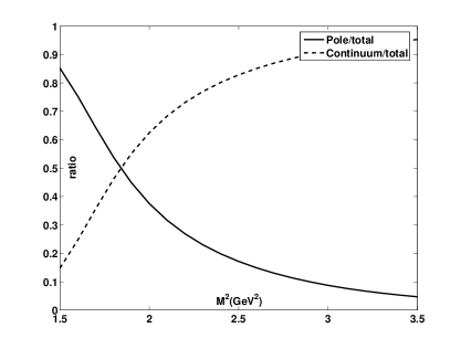
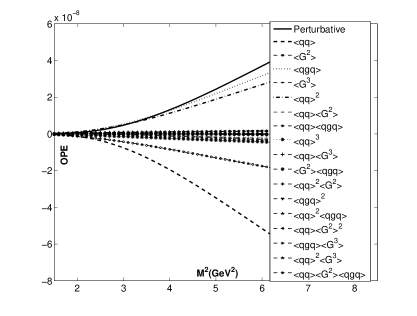
Figure 1: In the left panel, the solid line shows the relative pole contribution (the pole contribution divided by the total, pole plus continuum contribution) and the dashed line shows the relative continuum contribution from sum rule (10) for $\sqrt{s_{0}}=3.8~{}\mbox{GeV}$ for $D_{0}^{*}(2400)N$ state. The OPE convergence is shown by comparing the perturbative with other condensate contributions from sum rule (10) for $\sqrt{s_{0}}=3.8~{}\mbox{GeV}$ for $D_{0}^{*}(2400)N$ state in the right panel.

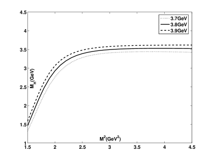
Figure 2: The mass of $D_{0}^{*}(2400)N$ state as a function of $M^{2}$ from sum rule (12) is shown. The continuum thresholds are taken as $\sqrt{s_{0}}=3.7\sim 3.9~{}\mbox{GeV}$.

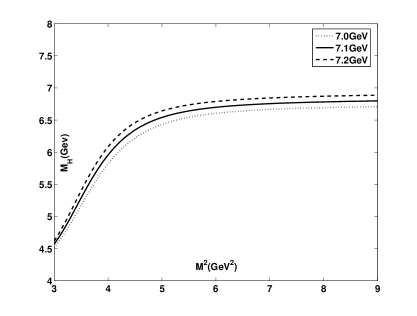
Figure 3: The mass of $\bar{B}_{0}^{*}N$ state as a function of $M^{2}$ from sum rule (12) is shown. The continuum thresholds are taken as $\sqrt{s_{0}}=7.0\sim 7.2~{}\mbox{GeV}$.

All in all, to test the OPE convergence, we have considered the ratio of the perturbative to the “total OPE contribution” instead of the ratio of the perturbative to each condensate contribution. This treatment is not freewheeling but has some definite constraints (i.e. there are merely few important condensates and they could cancel out each other to some extent; other condensates are almost negligible). In this sense, one could expect that the OPE convergence is still under control. We must truthfully admit that it is not a so good OPE convergence as the conventional case, but then one could find a comparatively reasonable work window and extract the hadronic information from QCD sum rules reliably. Thus, we choose some transition range $2.0\sim 3.0~{}\mbox{GeV}^{2}$ as a compromise Borel window and take the continuum thresholds as $\sqrt{s_{0}}=3.7\sim 3.9~{}\mbox{GeV}$, and arrive at $3.18\pm 0.41~{}\mbox{GeV}$ for $D_{0}^{*}(2400)N$ state. Considering the uncertainty rooting in the variation of quark masses and condensates, we gain $3.18\pm 0.41\pm 0.10~{}\mbox{GeV}$ (the first error reflects the uncertainty due to variation of $\sqrt{s_{0}}$ and $M^{2}$, and the second error resulted from the variation of QCD parameters) or $3.18\pm 0.51~{}\mbox{GeV}$ for $D_{0}^{*}(2400)N$ state.

On account of the difficulty encountered in finding a conventional Borel window, one may suppose the nonexistence of $D^{*}_{0}(2400)N$ molecule itself. As one possibility, the assumption of its nonexistence indeed should be drawn attention. However, in the present work, we are inclined to make a premise that the $D^{*}_{0}(2400)N$ molecular state could exist and then study whether it could act as one potential explanation of $X_{c}(3250)$ in view of two mian points: I) The possibility for the existence of $D_{0}^{*}(2400)N$ molecule and the molecular interpretation of $X_{c}(3250)$ are not entirely fabricated without any grounds. By an effective Lagrangian calculation X-th , He et al. found that $D_{0}^{*}(2400)$ and nucleon can form a loosely bound state with the small binding energy, and $X_{c}(3250)$ can be well explained as the $D_{0}^{*}(2400)N$ molecular hadron, which is supported by both the analysis of the mass spectrum and the study of its dominant decay channel. Moreover, the observed $X_{c}(3250)\rightarrow\Sigma_{c}^{++}\pi^{-}\pi^{-}$ can also be reasonably described. II) We believe the present result from QCD sum rules could provide another support to the $D_{0}^{*}(2400)N$ explanation to $X_{c}(3250)$. Certainly, we must confess to a weakness that it is difficult to find the conventional Borel window in the present case. Just as we have stated above, one could try releasing the rigid OPE convergence criterion and eventually find the OPE convergence is still under control in the present case. Although it is not a so good OPE convergence as the conventional case, one could find a comparatively reasonable work window and safely extract the hadronic information from QCD sum rules.

There comes forth the same problem for $\bar{B}_{0}^{*}N$ as the above case for $D_{0}^{*}(2400)N$, and we treat it similarly. The mass of $\bar{B}_{0}^{*}N$ state as a function of $M^{2}$ from sum rule (12) is shown in FIG. 3. Graphically, one can see there have very stable plateaus for Borel curves. We choose a compromise Borel window $4.5\sim 6.0~{}\mbox{GeV}^{2}$ and take $\sqrt{s_{0}}=7.0\sim 7.2~{}\mbox{GeV}$ for $\bar{B}_{0}^{*}N$ state. In the work windows, we obtain $6.50\pm 0.29~{}\mbox{GeV}$ for $\bar{B}_{0}^{*}N$ state. Varying input values of quark masses and condensates, we attain $6.50\pm 0.29\pm 0.20~{}\mbox{GeV}$ (the first error reflects the uncertainty due to variation of $\sqrt{s_{0}}$ and $M^{2}$, and the second error resulted from the variation of QCD parameters) or $6.50\pm 0.49~{}\mbox{GeV}$ for $\bar{B}_{0}^{*}N$ state.

IV Summary and outlook

Assuming the newly observed structure $X_{c}(3250)$ by BaBar Collaboration as a $D_{0}^{*}(2400)N$ molecular state, we calculate its mass value in the framework of QCD sum rules. Technically, contributions of operators up to dimension $12$ are included in the OPE. We find that it is difficult to find the conventional OPE convergence in this work. Via trying releasing the rigid OPE convergence criterion, one could find that the OPE convergence is still under control in the present work and the final numerical result for $D_{0}^{*}(2400)N$ state is $3.18\pm 0.51~{}\mbox{GeV}$, which coincides with the experimental value $3.25~{}\mbox{GeV}$. In view of that the conventional OPE convergence is not obtained here, thus only weak conclusions can be drawn regarding the explanation of $X_{c}(3250)$ in terms of a $D_{0}^{*}(2400)N$ molecular state. Meanwhile, one should note that the $D^{*}_{0}(2400)N$ molecular state is just one possible theoretical interpretation of $X_{c}(3250)$ and there may have some other different explanations for its configuration. One could expect that contributions from both future experimental observations and theoretical analysis will further reveal the nature structure of $X_{c}(3250)$. Additionally, we have also studied the bottom counterpart $\bar{B}_{0}^{*}N$ state and predicted its mass to be $6.50\pm 0.49~{}\mbox{GeV}$. By analogy with $D_{0}^{*}(2400)N$ state, this bottom counterpart state could be searched in the $\Sigma_{b}\pi^{-}\pi^{-}$ invariant mass spectrum in future experiments.

References

• (1) J. P. Lees et al., (BaBar Collaboration), Phys. Rev. D 86, 091102(R) (2012).
• (2) J. He, D. Y. Chen, and X. Liu, Eur. Phys. J. C 72, 2121 (2012).
• (3) M. B. Voloshin and L. B. Okun, JETP Lett. 23, 333 (1976).
• (4) A. D. Rujula, H. Georgi, and S. L. Glashow, Phys. Rev. Lett. 38, 317 (1977).
• (5) N. A. Törnqvist, Z. Phys. C 61, 525 (1994).
• (6) F. E. Close and P. R. Page, Phys. Lett. B 578, 119 (2004).
• (7) M. B. Voloshin, Phys. Lett. B 579, 316 (2004).
• (8) C. Y. Wong, Phys. Rev. C 69, 055202 (2004).
• (9) E. S. Swanson, Phys. Lett. B 588, 189 (2004).
• (10) N. A. Törnqvist, Phys. Lett. B 590, 209 (2004).
• (11) J. R. Zhang and M. Q. Huang, Commun. Theor. Phys. 54, 1075 (2010).
• (12) Y. L. Ma, Phys. Rev. D 82, 015013 (2010).
• (13) X. Liu, X. Q. Zeng, and X. Q. Li, Phys. Rev. D 72, 054023 (2005).
• (14) C. Z. Yuan, P. Wang, and X. H. Mo, Phys. Lett. B 634, 399 (2006).
• (15) J. L. Rosner, Phys. Rev. D 76, 114002 (2007).
• (16) C. Meng and K. T. Chao, arXiv:0708.4222; X.  Liu, Y. R. Liu, W. Z. Deng, and S. L. Zhu, Phys. Rev. D 77, 034003 (2008).
• (17) A. E. Bondar, A. Garmash, A. I. Milstein, R. Mizuk, and M. B. Voloshin, Phys. Rev. D 84, 054010 (2011).
• (18) D. Y. Chen, X. Liu, and S. L. Zhu, Phys. Rev. D 84, 074016 (2011).
• (19) K. P. Khemchandani, A. Martínez Torres, and E. Oset, Eur. Phys. J. A 37, 233 (2008); A. Martínez Torres, K. P. Khemchandani, and E. Oset, Phys. Rev. C 77, 042203(R) (2008); D. Gamermann, C. García-Recio, J. Nieves, and L. L. Salcedo, Phys. Rev. D 84, 056017 (2011); O. Romanets, L. Tolos, C. García-Recio, J. Nieves, L. L. Salcedo, and R. G. E. Timmermans, Phys. Rev. D 85, 114032 (2012).
• (20) M. A. Shifman, A. I. Vainshtein, and V. I. Zakharov, Nucl. Phys. B147, 385 (1979); B147, 448 (1979); V. A. Novikov, M. A. Shifman, A. I. Vainshtein, and V. I. Zakharov, Fortschr. Phys. 32, 585 (1984).
• (21) B. L. Ioffe, in The Spin Structure of The Nucleon, edited by B. Frois, V. W. Hughes, and N. de Groot (World Scientific, Singapore, 1997).
• (22) S. Narison, Camb. Monogr. Part. Phys. Nucl. Phys. Cosmol. 17, 1 (2002).
• (23) P. Colangelo and A. Khodjamirian, in At the Frontier of Particle Physics: Handbook of QCD, edited by M. Shifman, Boris Ioffe Festschrift Vol. 3 (World Scientific, Singapore, 2001), pp. 1495-1576; A. Khodjamirian, Continuous Advances in QCD 2002/ARKADYFEST.
• (24) M. Neubert, Phys. Rev. D 45, 2451 (1992); M. Neubert, Phys. Rep. 245, 259 (1994).
• (25) M. Nielsen, F. S. Navarra, and S. H. Lee, Phys. Rep. 497, 41 (2010).
• (26) S. L. Zhu, Phys. Rev. Lett 91, 232002 (2003); R. D. Matheus, F. S. Navarra, M. Nielsen, R. Rodrigues da Silva, and S. H. Lee, Phys. Lett. B 578, 323 (2004); J. Sugiyama, T. Doi, and M. Oka, Phys. Lett. B 581, 167 (2004); M. Eidemuller, Phys. Lett. B 597, 314 (2004); Z. G. Wang, W. M. Yang, and S. L. Wan, Phys. Rev. D 72, 034012 (2005).
• (27) H. Kim, S. H. Lee, and Y. Oh, Phys. Lett. B 595, 293 (2004).
• (28) J. R. Zhang and M. Q. Huang, Phys. Rev. D 77, 094002 (2008); Phys. Rev. D 78, 094007 (2008); Phys. Lett. B 674, 28 (2009); Phys. Rev. D 80, 056004 (2009); J. Phys. G: Nucl. Part. Phys. 37, 025005 (2010); J. R. Zhang, M. Zhong, and M. Q. Huang, Phys. Lett. B 704, 312 (2011).
• (29) L. J. Reinders, H. R. Rubinstein, and S. Yazaki, Phys. Rep. 127, 1 (1985).
• (30) B. L. Ioffe, Nucl. Phys. B 188, 317 (1981); E. V. Shuryak, Nucl. Phys. B 198, 83 (1982).
• (31) R. D. Matheus, F. S. Navarra, M. Nielsen, and R. Rodrigues da Silva, Phys. Rev. D 76, 056005 (2007).
• (32) J. R. Zhang, L. F. Gan, and M. Q. Huang, Phys. Rev. D 85, 116007 (2012); J. R. Zhang and G. F. Chen, Phys. Rev. D 86, 116006 (2012).