Two-dimensional electronic transport on the surface of 3D topological insulators

Abstract

We present a theoretical approach to describe the 2D transport properties of the surfaces of three dimensional topological insulators (3DTIs) including disorder and phonon scattering effects. The method that we present is able to take into account the effects of the strong disorder-induced carrier density inhomogeneities that characterize the ground state of the surface of 3DTIs, especially at low doping, as recently shown experimentally. Due to the inhomogeneous nature of the carrier density landscape, standard theoretical techniques based on ensemble averaging over disorder assuming a spatially uniform average carrier density are inadequate. Moreover the presence of strong spatial potential and density fluctuations greatly enhance the effect of thermally activated processes on the transport properties. The theory presented is able to take into account all the effects due to the disorder-induced inhomogeneities, momentum scattering by disorder, and the effect of electron-phonon scattering processes. As a result the developed theory is able to accurately describe the transport properties of the surfaces of 3DTIs both at zero and finite temperature.

I Introduction

In strong three dimensional topological insulators (3DTIs) the nontrivial topology of the bulk energy bands HasanKane_RMP10 ; FKM_PRL07 ; Culcer_PhysicaE2011 enforces the essential existence of 2D metallic surface states that can be well described at low energies as massless Dirac fermions. The valence and conduction band of the surface states touch at isolated points, the Dirac points, whereas the bulk states are gapped. Angle resolved photo-emission spectroscopy experiments have confirmed the existence of the Dirac like surface states in Bi_1-xSb_xHsieh_Nature08 , Bi₂Se₃Hasan_NPH09 ; Hsieh_Nature09 , Bi₂Te₃chen_science_2009 ; Hsieh_PRL09 and Sb₂Te₃Hsieh_PRL09 . Electronically, the surface of a 3DTI is very analogous to graphene novoselov2004 ; dassarma2011 in which the fermionic excitations are also well described, at low energies, as massless Dirac fermions. There are two fundamental differences between graphene and the surfaces of 3DTIs: (i) In graphene the chiral nature is due to the locking of the momentum direction with the electron pseudospin, associated with the sublattice degree of freedom, instead of the real spin as in the surface of strong 3DTIs; (ii) In strong 3DTIs the number of Dirac points is odd whereas in graphene is even. These differences make graphene and the surfaces of strong 3DTIs fundamentally different. However, the fact that graphene and the surfaces of strong 3DTIs are both two-dimensional electronic systems and have a very similar band structure suggests that these two systems might have similar charge-transport properties. As we show in this work this is only partially correct.

Two important aspects of TI surface transport need to be mentioned (in the context of our comprehensive theoretical work to be presented in this paper) so as to avoid any confusion about our goal and scope. First, 2D TI transport occurs on the surface of 3D TI materials, and theoretically the bulk 3D states should be insulating with no metallic contribution to the conductivity. Experimentally, however, this situation of 2D metallic transport on a bulk 3D insulator has not yet been achieved since the bulk, instead of being a band insulator, seems to have a lot of free carriers which contribute (indeed, often dominate) the measured conductivityButch_PRB10 . We completely ignore the complications of the bulk conduction and the bulk carriers in our theory concentrating entirely on purely the 2D surface conductivity (as a function of density and temperature) assuming the bulk to be an insulator as the theory implies it should be. Recent experimental advances in materials preparation and thin film device fabrication have made it possible to see the expected pure 2D surface conduction with little contamination from the bulk states, and thus, our work is relevant to an increasing body of recent dataDohun_arXiv11 ; Hong_arXiv11 ; Kong_Natnano ; Steinberg_PRB11 . In any case, the subject is interesting only because of the 2D metallic surface topological states, and therefore, we focus entirely on this issue. Second, the actual energy dispersion of the 3DTI surface states appears to follow the linear Dirac-like spectrum only at rather low energies, particularly for the hole states (i.e. the valence band) with strong nonlinearity becoming apparent at higher energies. This nonlinearity (e.g. a quadratic correction to the linear dispersion) is nonuniversal and strongly materials-dependent whereas the theoretical Dirac-behavior at low energies is universal (with different Fermi velocities characterizing different TI materials). Because the focus of our work is on the universal behavior arising from density inhomogeneity (which is much more important at low Fermi energies, i.e. low 2D densities), which should not depend much on the details of the band structure at higher energies, we ignore the higher energy parabolicity of the 2D surface bands. We emphasize that these two approximations, neglect of bulk conduction and surface band dispersion correction at higher energy, imply that our theory should not be construed as a quantitative theory for any particular TI material, but as a qualitative guide for the universal features of 3DTI surface transport behavior. Detailed quantitative comparison between theory and experiments is further complicated by our lack of knowledge of the precise parameters for TI systems any way (e.g. the Fermi velocity, the phonon parameters, the nature of disorder, etc.), and therefore, our theory provides the zeroth order qualitative theory for 3DTI surface transport which should apply to all TI materials.

The surfaces of the newly discovered strong 3DTIs are of great fundamental interestWilczek_PRL87 ; qxl_PRB08 ; Wilczek_Nat09 ; rli_natphy10 and in addition have the potential to be used in disruptive novel technologies such as topological quantum information processingFuKane_PRL08 ; FuKane_PRB09 ; JMoore_Nature10 . To be able to use the surfaces of 3DTIs to study novel fundamental phenomena and in novel technologies it is essential to understand their electron transport properties and in particular to understand the main factors limiting their electron mobility. Recently, experiments on thin films of strong 3DTIs Dohun_arXiv11 ; Hong_arXiv11 ; Kong_Natnano ; Steinberg_PRB11 , by enhancing the surface-to-volume ratioLiuMinhao_PRB11 , have been able to greatly reduce the bulk contribution transport and obtain the intrinsic 2D transport properties of the surfaces of strong 3DTIs. Previous theoretical works on the transport in the surface of strong 3DTIs Culcer_TIPRB10 ; Adam_arXiv12 have used simplified models and have mostly focused on the zero temperature limit.

In this work we present a comprehensive transport theory for the surfaces of 3DTIs valid both at zero temperature and at finite temperatures. As in graphene Martin_NP08 ; YZhang_NP09 , one of the main difficulties in developing a transport theory for the surfaces of 3DTIs is the presence, especially at low doping, of strong carrier density inhomogeneities Beidenkopf_NPH11 induced by disorder. The presence of strong spatial fluctuations makes the standard theoretical approaches, that rely on the homogeneous nature of the ground state, inadequate. Moreover, because of the inhomogeneities, at finite temperatures the contribution of thermally activated carriers to transport can be very important and difficult to quantify. Thus, disorder-induced density inhomogeneity by itself could introduce considerable insulating-like activated transport behavior in the nominally metallic 3DTI surface conduction. The transport theory that we present takes into account both the effects of quenched disorder and electron-phonon scattering processes. In particular our theory is able to take into account the effects of the strong disorder-induced inhomogeneities both at zero and finite temperature.

To characterize the inhomogeneous ground state we generalize to the case of 3DTIs’ surfaces the Thomas-Fermi-Dirac-Theory (TFDT) first developed to study graphene rossi2008 ; dassarma2011 . Combining the TFDT results and the Boltzmann theory we develop and validate the effective medium theory (EMT) to obtain the transport properties at zero temperature. We then develop an effective 2-fluid transport theory that we validate at zero temperature by comparing its results to the ones obtained using the EMT. The great advantage of the 2-fluid theory is that it allows to readily obtain the transport properties at finite temperature including all the temperature dependent effects: electron-phonon scattering, thermal activation, changes with temperature of the screening properties, and thermal broadening of the Fermi surface. Given the experimental evidence Dohun_arXiv11 ; Hatch_PRB11 that in current 3DTIs charged impurities are the dominant source of disorder we have applied the theory to the case in which the quenched disorder is due to random charges placed in the vicinity of the surface of the 3DTI. We provide both a detailed analytical theory and comprehensive numerical results for the density and temperature dependent 3DTI surface transport properties in the presence of density inhomogeneity, scattering by random charged impurities, and phonon scattering.

In section II we present the theoretical approach that we have developed to describe the transport on the surfaces of 3DTIs taking into account both quenched disorder and electron-phonon scattering processes, in particular when the quenched disorder is due to charged impurities. In section III.1 we present our results for the characterization of the disorder-induced carrier density inhomogeneities obtained using the TFDT. In section III.2 we present our results for the conductivity at zero temperature and finally in section III.3 we present our results for the conductivity at finite temperature. Section IV briefly summarizes our findings and the differences between the 2D transport properties of the surfaces of 3DTIs and single layer graphene.

II Theoretical approach

To study the electronic transport on the surface of strong 3DTIs we use the Boltzmann theory. From the Boltzmann theory, within the “relaxation time approximation”, the electronic conductivity $\sigma$ is given by the following equation:

$$\sigma(n,T)=\frac{e^{2}}{2}\int d\epsilon D(\epsilon)v_{F}^{2}\tau_{tot}(\epsilon,T)\left(-\frac{\partial f(\epsilon)}{\partial\epsilon}\right)$$ (1)

where $e$ is the electron charge, $D(\epsilon)$ the density of states at energy $\epsilon$, $v_{F}$ the Fermi velocity, $f(\epsilon)=1/(1+e^{\beta(\epsilon-\mu)})$ the Fermi-Dirac distribution, and $\tau_{tot}$ the total transport mean free time due to the electron scattering off quenched disorder and phonons. Assuming independent scattering from disorder and phonons (we mention that this is not equivalent to assuming the Matthiessen’s rule which assumes that the resistivity due to independent mechanisms can be added and is invalid for our system) we have

$$\frac{1}{\tau_{tot}}=\frac{1}{\tau_{dis}}+\frac{1}{\tau_{ph}}$$ (2)

where $\tau_{dis}$ is the transport mean free time due to electrons scattering off quenched disorder and $\tau_{ph}$ is the transport mean free time due to electron-phonon scattering processes. One thing that we must emphasize is that Eq. (1) is valid as long as the system is homogeneous (i.e. spatial density fluctuations effects are small enough so that the average density $n$ is a meaningful quantity, an approximation which would break down for low $n$).

The energy dependent scattering time $\tau_{dis}(\epsilon)$ due to quenched disorder is given by

$$\dfrac{\hbar}{\tau_{dis}(\epsilon_{p{\bf k}})}=2\pi n_{dis}\int\frac{d^{2}k^{\prime}}{(2\pi)^{2}}|\langle V_{p{\bf k},p{\bf k^{\prime}}}\rangle|^{2}g(\theta_{\bf kk^{\prime}})$$

$$\times\left[1-\cos\theta_{\bf kk^{\prime}}\right]\delta(\epsilon_{p\mathbf{k^{\prime}}}-\epsilon_{p\mathbf{k}})$$ (3)

where $\epsilon_{p\mathbf{k}}=p\hbar v_{F}|\mathbf{k}|$ is the energy of a quasiparticle with $p=\pm 1$ and momentum ${\bf k}$, $n_{dis}$ is the 2D density of impurities, $\langle V_{p{\bf k},p{\bf k^{\prime}}}\rangle$ is the matrix element of the scattering potential, $g(\theta_{\bf kk^{\prime}})=\left[1+\cos\theta_{\bf kk^{\prime}}\right]/2$ is the TI chiral matrix element factor arising from the wavefunction overlap between states with momentum ${\bf k}$ and momentum ${\bf k}^{\prime}$ with $\theta_{\bf kk^{\prime}}$ the angle between ${\bf k}$ and ${\bf k}^{\prime}$. In Eq. (3), to minimize the number of parameters entering the theory we have assumed that the impurities are randomly distributed in a 2D plane located at an effective distance $d$ from the surface of the 3DTI. It is straightforward to include in the theory a more complex three-dimensional distribution of quenched impurities, but given the lack of experimental information about the distribution of unintentional and unknown quenched impurity disorder in the system, it is theoretically more meaningful to use a minimal model with just two unknown parameters $n_{dis}$ and $d$, which can simulate essentially any realistic disorder distribution in an approximate manner– we note that $d=0$ implies that the charged impurities are simply located on the surface of the 3DTI.

There is considerable evidence Dohun_arXiv11 that in 3DTIs random unintentional charged impurities are the dominant source of disorder scattering. We therefore assume that the quenched disordered potential $V_{D}$ is due to charged impurities. For charged impurities, taking into account screening by the 2D surface carriers themselves in addition to the screening by the background lattice, we have $n_{dis}|\langle V_{p{\bf k},p{\bf k^{\prime}}}\rangle|^{2}=n_{imp}|v_{i}(q)/\varepsilon(q,T)|^{2}$ where $v_{i}(q)=2\pi e^{2}/(\kappa q)$ is the Fourier transform of the 2D Coulomb potential in a medium with an effective background static lattice dielectric constant $\kappa$, and $\varepsilon(q,T)$ is the 2D static RPA dielectric function at finite temperatureHwangDas_PRB07 . The reported values of $\kappa$ for Bi₂Se₃ range from 30, Ref. Beidenkopf_NPH11, , to $\approx 55$, Ref. Butch_PRB10, .

In Bi₂Se₃ the lowest optical phonon energy has been measured to be $8.94$ meV$\approx 100$ K Kumar_PRB11 ; Richter_PSS77 and therefore the optical phonons provide a substantial source of scattering only at high temperature ($\gtrsim 250~{}K$) kim2012 . Because we are interested primarily only in the transport properties at temperatures below 250 K in the remainder we neglect the contribution to the resistivity due to optical phonons and consider only the contribution due to acoustic phonons.

Following references Hwang_phononPRB08, ; Giraud_PRB11, ; Giraud_PRB12, we have that, considering only longitudinal acoustic phonons, the scattering time $\tau_{ph}$ is given by

$$\frac{1}{\tau_{ph}(\varepsilon)}=\sum_{{\bf k}^{\prime}}(1-\cos\theta_{{\bf k}{\bf k}^{\prime}})W_{{\bf k}{\bf k}^{\prime}}\frac{1-f(\varepsilon^{\prime})}{1-f(\varepsilon)},$$ (4)

where

$$W_{{\bf k}{\bf k}^{\prime}}=\frac{2\pi}{\hbar}\sum_{{\bf q}}|C({\bf q})|^{2} \times [N_{q}\delta(\varepsilon-\varepsilon^{\prime}+\omega_{{\bf q}})$$ (5)

$$+ (N_{q}+1)\delta(\varepsilon-\varepsilon^{\prime}-\omega_{{\bf q}})],$$

is the transition probability from the state with momentum ${\bf k}$ to the state with momentum ${\bf k}^{\prime}$. In (5) ${\bf q}={\bf k}-{\bf k}^{\prime}$, $C({\bf q})$ is the matrix element for scattering by acoustic phonon, $\omega_{{\bf q}}=v_{l}{\bf q}$ is the acoustic phonon frequency with $v_{l}$ the phonon velocity, and $N_{q}={1}/({\exp(\beta\omega_{{\bf q}})-1})$ is the phonon occupation number. The matrix element $C({\bf q})$ for the deformation potential electron-phonon coupling is given by

$$|C({\bf q})|^{2}=\frac{D^{2}\hbar q}{2A\rho_{m}v_{l}}\left[1-\left(\frac{q}{2k}\right)^{2}\right]$$ (6)

where $D$ is the deformation potential coupling constant, $A$ is the area of the sample, and $\rho_{m}$ is the 2D mass density of one quintuple layer (around $1$ nm thick) of Bi₂Se₃, given that the length scale over which the 2D surface states decay into the bulk is approximately 1 nm LiuQiZh_PRB10 .

Using Eqs. (1)-(6) we can calculate the conductivity taking into account scattering events due to both quenched disorder and phonons as long as the system is homogeneous. However, especially close to the Dirac point, the random charged impurity induced disorder potential causes the carrier density landscape to become strongly inhomogeneous, a fact that has been observed experimentally in TIs Beidenkopf_NPH11 and previously in graphene Martin_NP08 ; YZhang_NP09 . To develop a theory in the presence of strong inhomogeneities it is first necessary to characterize them. To do this we use the Thomas-Fermi-Dirac-Theory (TFDT) first introduced in Ref. rossi2008, . In the TFDT, similarly to the Density Functional Theory (DFT), the energy of the system is given by a functional of the density profile $n({\bf r})$. The great advantage of a functional formalism is that it is not perturbative with respect to the spatial fluctuations of the carrier density and therefore can take into account nonlinear screening effects that dominate close to the Dirac point. TFDT is just well-suited to describe the situation with large disorder-induced spatial density inhomogeneity as in the low carrier density case whereas in the high-density situation, it simply gives the homogeneous density result with small fluctuations around the average density. In the TFDT, contrary to DFT, also the kinetic energy term is replaced by a density functional. This simplification makes the TFDT very efficient computationally and therefore able to obtain disorder averaged quantities, a task that cannot be accomplished using DFT. The simplification also makes the TFDT in general less accurate than DFT polini2008 , however as long as the characteristic length-scale over which the density varies is larger than the local Fermi wavelength $\lambda_{F}$, i.e. $|\nabla n/n|^{-1}\gg\lambda_{F}$, rossi2008 ; rossi2009 ; brey2009 the TFDT returns reliable results rossi2008 ; dassarma2009 ; rossi2011 . Our results show that as in graphene rossi2008 the condition $|\nabla n/n|^{-1}\gg\lambda_{F}$ is satisfied for the surface of 3DTIs in typical experimental conditions. Close to the charge neutrality point (CNP) the density inside the electron-hole puddles is always different from zero (so that $\lambda_{F}$ is always finite) and of the order of $n_{rms}$. Our results show that $n_{rms}\sim n_{imp}$ and therefore the TFDT is also valid at the CNP as long as $n_{imp}$ is not too small. The great advantage of TFDT over DFT (to which TFDT is an approximation, as it uses the non-interacting kinetic energy functional) is that its relative numerical and computational ease enables one to use it for the calculation of transport properties using the computed ground state inhomogeneous spatial density profile, which would be completely computationally impossible for DFT to do.

Using the TFDT we can characterize completely the carrier density profile in the presence of a disorder potential. We can obtain the typical length scale $L_{D}$ and root mean square fluctuation $n_{\rm rms}$ of the disorder-induced carrier density inhomogeneities. Using the Boltzmann theory we obtain the relation between the mean free path and the doping, $\ell(n)=v_{F}\tau_{tot}(n)$, valid in the homogeneous limit. In the limit in which $\ell(n_{\rm rms})\ll L_{D}$ the number of scattering events inside a single homogeneous region, puddle, of the inhomogeneous landscape is large enough that the Boltzmann theory is valid locally. In addition, due to the Klein tunneling, as in graphene fogler2008 ; beenakker2008 ; katsnelson2006b ; shytov2008 ; stander2009 ; young2009 ; rossi2010 , the resistance due to the boundaries between the puddles can be neglected in comparison to the resistance arising from scattering events inside the puddles rossi2009 . Under these conditions, due to the random distribution of the puddles, 2D transport on the surface of a 3DTI can be described by the effective medium theory (EMT) bruggeman1935 ; landauer1952 ; hori1975 ; rossi2009 ; fogler2009 ; dassarma2011 . In the EMT, which is extensively used in science and engineering to quantitatively describe properties of highly inhomogeneous systems, the conductivity of the inhomogeneous system is obtained as the conductivity $\sigma_{EMT}$ of an equivalent homogeneous effective medium by averaging over disorder realizations the local values $\sigma(n({\bf r}))$ given by the Boltzmann theory. The resulting implicit equation for $\sigma_{EMT}$ is:

$$\int dn\frac{\sigma(n)-\sigma_{EMT}}{\sigma(n)+\sigma_{EMT}}P[n]=0$$ (7)

where $P[n]$ is the disorder-averaged carrier density probability distribution that we obtain using the TFDT. A solution of the implicit EMT integral equation defined by Eq. 7 provides the effective conductivity of the inhomogeneous system. In graphene the TFDT+EMT method has been shown to give results in remarkable agreement with experiments dassarma2011 even in the highly inhomogeneous situation very close to the Dirac point and with full quantum transport analysis rossi2012 ; rossi2010 .

A simplified approach that allows to make further analytical progress and obtain results in qualitative agreement with the numerical TFDT-EMT approach is the “2-fluid” model qzli_MLGPRB11 . In this approach the inhomogeneous state characterized by the presence of electron-hole puddles is approximated as a system comprised of the “electron-fluid”, formed by the electrons, and the “hole-fluid” formed by the holes, with conductivity $\sigma_{e}$ and $\sigma_{h}$ respectively. Let $p$ be the fraction of the system occupied by the electron gas, and consequently $(1-p)$ the fraction occupied by the hole gas. Adapting Eq. (7) to the simple case of only two components for the inhomogeneous system we obtain the effective conductivity kirkpatrick1973 ; Hwang_InsuPRB2010 ; qzli_MLGPRB11 :

$$\sigma_{t}=(p-\frac{1}{2})\left[(\sigma_{e}-\sigma_{h})+\sqrt{(\sigma_{e}-\sigma_{h})^{2}+\frac{4\sigma_{e}\sigma_{h}}{(2p-1)^{2}}}\right].$$ (8)

One advantage of the 2-fluid model is that it allows to easily take into account the effect of activation processes that at finite temperature, especially close to the Dirac point, give a substantial contribution to the conductivity and in particular qualitatively modify its temperature dependence. Carrier activation becomes operational when local potential fluctuations due to weak screening at low density lead to carrier confinement or localization in puddles, and global transport involves thermal activation of carriers over the local potential hills and barriers. The activation process, which obviously becomes more important as the inhomogeneity becomes more important at lower carrier density, cannot be captured by the simple Boltzmann theory of Eq. (1) or, for that matter, by any ensemble-averaged transport theory. To take into account the presence of activation processes $\sigma_{e}$ and $\sigma_{h}$ can be written as a sum of two terms qzli_MLGPRB11 :

$$\sigma_{e} =\sigma_{e}^{(na)}+\sigma_{h}^{(a)}$$

$$\sigma_{h} =\sigma_{h}^{(na)}+\sigma_{e}^{(a)}$$

where $\sigma_{e}^{(na)}$, $\sigma_{h}^{(na)}$ are the disorder averaged conductivities obtained using the Boltzmann theory and $\sigma_{e}^{(a)}$, $\sigma_{h}^{(a)}$ the contribution to the conductivity from activation processes.

$\sigma_{e}^{(na)}$, ($\sigma_{h}^{(na)}$) can be obtained by multiplying Eq. (1) by the ratio $n_{e}/n_{0}$ ($n_{h}/n_{0}$)qzli_MLGPRB11 . Here, $n_{e}=\int_{-\infty}^{\infty}D_{e}(\epsilon)f(\epsilon)d\epsilon$ ($n_{h}=\int_{-\infty}^{\infty}D_{h}(\epsilon)[1-f(\epsilon)]d\epsilon$) denotes the effective electron (hole) density of inhomogeneous systems, while $n_{0}=\int_{0}^{\infty}\frac{g_{s}g_{v}\epsilon}{2\pi(\hbar v_{F})^{2}}f(\epsilon)d\epsilon$ is the electron density of homogeneous systems. The density of states $D_{e}(\epsilon)$ ($D_{h}(\epsilon)$) after disorder averaging are given byqzli_MLGPRB11 :

$$D_{e}(\epsilon) =\int_{-\infty}^{\epsilon}\frac{g_{s}g_{v}(\epsilon-V)}{2\pi(\hbar v_{F})^{2}}P(V)dV$$

$$D_{h}(\epsilon) =\int_{\epsilon}^{\infty}\frac{g_{s}g_{v}(V-\epsilon)}{2\pi(\hbar v_{F})^{2}}P(V)dV$$

where $P(V)$ is the probability distribution of the screened disorder potential. We want to mention that we use the density of states for homogeneous systems in Eq. (1), i.e., $D(\epsilon)=\frac{g_{s}g_{v}\epsilon}{2\pi(\hbar v_{F})^{2}}$, to avoid double counting since the density inhomogeneity effects have already been considered through the variation of effective carrier density. At higher doping, both $n_{e}/n_{0}$ and the fraction of area occupied by electrons, denoting as $p=\int_{-\infty}^{E_{F}}P(V)dV$, approach unity while $n_{h}/n_{0}$ approaches zero. Note, however, that the ratio $n_{e}/n_{0}$ ($n_{h}/n_{0}$) being temperature-dependent is generally not equal to $p$ ($(1-p)$). Given that the 2-fluid model is an effective model the use of the exact $P(V)$ does not guarantee an increase of its accuracy. It is more sensible to simply assume $P(V)$ to have an effective Gaussian profile

$$P(V)=\frac{1}{\sqrt{2\pi s^{2}}}\exp(-V^{2}/2s^{2}).$$ (9)

with effective variance $s^{2}$. The TFDT results, presented in Sec. III, show that the root mean square $s$ of the screened disorder potential depends weakly on the doping or carrier density. In Eq. 9 we can then neglect the dependence of $s$ on the average doping and use the value obtained for the Dirac point. We consider two ways to estimate the value of the effective $s$ at the Dirac point that enters the Gaussian approximation for $P(V)$: (i) the self-consistent approximation introduced in Ref. adam2007, ; (ii) the quasi-TFDT approximation in which $s$ is fixed using the relation between $n_{\rm rms}$ and $s$ in the Thomas-Fermi approximation with the value of $n_{\rm rms}$ obtained from the full TFDT calculation.

In general $P(V)$ cannot be obtained analytically but it is possible to obtain explicit expression for its moments galitski2007 . For the second moment $\langle(\delta V)^{2}\rangle$ taking into account screening effects, within the random-phase-approximation (RPA) for the surface states of a 3DTI with total degeneracy $g=g_{s}g_{v}=1$ we have galitski2007 :

$$\langle(\delta V)^{2}\rangle=2\pi n_{imp}\left(\frac{e^{2}}{\kappa}\right)^{2}C_{0}(r_{s},a=k_{F}d)$$ (10)

where

$$C_{0}(r_{s},a) = -1+\frac{e^{-4a}r_{s}}{2+r_{s}}+\frac{64E_{1}[4a]}{(8+\pi r_{s})^{2}}$$

$$+ e^{2r_{s}a}(1+2r_{s}a)(E_{1}[2r_{s}a]-E_{1}[4a+2r_{s}a]),$$

$r_{s}\equiv e^{2}/(\hbar v_{F}\kappa)$, and $E_{1}[z]=\int_{z}^{\infty}t^{-1}e^{-t}dt$ is the exponential integral function. Assuming $P(V)$ to be a Gaussian with variance $s^{2}$ we have $s^{2}=\langle(\delta V)^{2}\rangle$. The difficulty arises from the fact that the function $C_{0}$ depends on the density via the Fermi wavevector $k_{F}$ that, in the presence of disorder, at the Dirac point cannot, because of fluctuations, be taken to be simply zero. In the self-consistent approximation one assumes that at the Dirac point the system can be approximated by a homogeneous system having an effective carrier density $\hat{n}=(g/4\pi)\hat{k}_{F}^{2}$ such that $\hat{E}_{F}^{2}=s^{2}$, i.e. $\hbar^{2}v_{F}^{2}k_{F}^{2}=s^{2}$. Using this relation and Eq. (10) we obtain the following self-consistent equation for $s$:

$$s^{2}=2\pi n_{imp}\left(\frac{e^{2}}{\kappa}\right)^{2}C_{0}(r_{s},a=sd/(\hbar v_{F})).$$ (12)

By solving Eq. (12) we obtain the value of $s$ within the self-consistent approximation. In the self-consistent+2-fluid model the variance of the effective Gaussian probability distribution $P(V)$ is obtained using Eq. (12).

By minimizing the Thomas-Fermi energy functional, at the Dirac point, for $g=1$, we obtain the following equation

$$2\hbar v_{F}\operatorname{sgn}(n)\left(\frac{\pi|n({\bf r})|}{g_{s}g_{v}}\right)^{1/2}-V({\bf r})=0$$ (13)

where the first term is due to the kinetic energy and $V({\bf r})$ is the local value of the screened disorder potential. By disorder averaging (13) and assuming $P(V)$ to be a Gaussian with variance $s^{2}$ we obtain

$$n_{\rm rms}=\frac{g_{s}g_{v}}{2\pi(\hbar v_{F})^{2}}\frac{\sqrt{3}}{4}s^{2}.$$ (14)

In the quasi-TFDT approximation the value of $s$ used in the 2-fluid model is set using Eq. (14) and the value of $n_{\rm rms}$ obtained from the TFDT at the Dirac point.

Locally, the activated conductivities $\sigma_{e}^{(a)}$, $\sigma_{h}^{(a)}$ are given by:

$$\sigma_{e}^{(a)}(V({\bf r})) =\sigma_{e}^{(na)}\exp[\beta(E_{F}-V({\bf r}))]$$ (15)

$$\sigma_{h}^{(a)}(V({\bf r})) =\sigma_{h}^{(na)}\exp[\beta(V({\bf r})-E_{F})].$$ (16)

where $V({\bf r})$ is the local value of the screened disorder potential. By disorder averaging these expressions and summing the contribution of the non-activated conductivities we finally find qzli_MLGPRB11 :

$$\sigma_{e} = \frac{1}{p}\int^{E_{F}}_{-\infty}(\sigma_{e}^{(na)}+\sigma_{h}^{(a)})P(V)dV,$$ (17)

$$= \sigma_{e}^{(na)}+\frac{\sigma_{h}^{(na)}}{2p}e^{\frac{\beta^{2}s^{2}}{2}-\beta E_{F}}{\rm erfc}\left(-\frac{E_{F}}{\sqrt{2}s}+\frac{\beta s}{\sqrt{2}}\right).$$

$$\sigma_{h} = \frac{1}{(1-p)}\int_{E_{F}}^{\infty}(\sigma_{h}^{(na)}+\sigma_{e}^{(a)})P(V)dV$$ (18)

$$= \sigma_{h}^{(na)}+\frac{\sigma_{e}^{(na)}}{2(1-p)}e^{\frac{\beta^{2}s^{2}}{2}+\beta E_{F}}{\rm erfc}\left(\frac{E_{F}}{\sqrt{2}s}+\frac{\beta s}{\sqrt{2}}\right).$$

where the fraction of the system occupied by electrons is given by $p=\int_{-\infty}^{E_{F}}P(V)dV$ with Fermi energy $E_{F}$. These are the expressions of the electron and hole conductivities that enter the 2-fluid model whose total conductivity $\sigma_{t}$ is then obtained by using Eq. (8). We notice that in the expressions (17), (18) several temperature effects are taken into account: (i) the effect due to electron-phonon scattering processes that affect the total scattering time and therefore the value of $\sigma_{e}^{(na)}$ and $\sigma_{h}^{(na)}$; (ii) the temperature dependence of the dielectric functions that enters in the calculation of $\tau_{dis}$ and that affect the value of $\sigma_{e}^{(na)}$ and $\sigma_{h}^{(na)}$; (iii) the thermal broadening of the Fermi surface; (iv) the presence of thermal activation. The ability to capture all these effects makes the 2-fluid model a very useful tool to study the transport properties of disordered TIs.

It is useful to explicitly write down the expression for the conductivity $\sigma_{CNP}$ at the charged neutrality point obtained using the 2-fluid model. At the CNP we have that 50% of the sample will be covered by electron puddles and 50% by hole puddles so that $p=1-p=0.5$. In this case $\sigma_{t}=\sigma_{e}=\sigma_{h}$. At zero temperature, there are no thermal activation effects and we find qzli_MLGPRB11 :

$$\sigma_{CNP}=\sigma^{(na)}_{CNP}=\frac{1}{8G[r_{s}/2]}\frac{e^{2}}{h}\frac{g_{s}g_{v}}{2\pi(\hbar v_{F})^{2}}\frac{s^{2}}{4n_{imp}}$$ (19)

where

$$\frac{G[x]}{x^{2}}=\frac{\pi}{4}+3x-\frac{3\pi x^{2}}{2}+\frac{x(3x^{2}-2)\arccos[1/x]}{\sqrt{x^{2}-1}}$$ (20)

Using Eq. (14) we can rewrite (19) in terms of $n_{\rm rms}$:

$$\sigma^{(na)}_{CNP}=\frac{1}{8G[r_{s}/2]}\frac{e^{2}}{h}\frac{n_{\rm rms}}{\sqrt{3}n_{imp}}$$ (21)

In the following sections we present our results and in particular, when possible, a comparison between the three approaches introduced: TFDT+EMT approach, quasi-TFDT+2-fluid model, and self-consistent+2-fluid model.

III Results

III.1 TFDT results

In this section we present the results for the carrier density distribution. These results will then be used to calculate the conductivity within the EMT and the 2-fluid models.

In Fig. 1, we show the carrier density profile calculated using the TFDT for a single disorder realization with charged impurity density $n_{imp}=7.5\times 10^{13}$ cm^-2 and two different values for the impurity distances, $d=0.1$ nm, and $d=0.2$ nm in panel (a) and (b) respectively. Unless otherwise specified, we use the background dielectric constant $\kappa=50$ for Bi₂Se₃ and the Fermi velocity $v_{F}=6.4\times 10^{5}$ m/s zhang2009ti ; Dohun_arXiv11 .

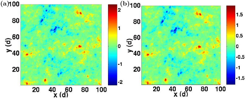
Figure 1: (Color online). Color plots of carrier density distribution $n(\mathbf{r})$ at the Dirac point for $n_{imp}=7.5\times 10^{13}$ cm^-2 and $\kappa=50$. The color-scale is in units of $10^{13}$ cm^-2. (a) The impurity distance $d=0.1$ nm. (b) The impurity distance $d=0.2$ nm.

Figure 1 conveys the nature of the carrier density landscape on the surface of disordered 3DTIs as also shown recently by direct imaging experiments Beidenkopf_NPH11 . To be able to make a quantitative comparison with the experiments, and calculate the conductivity for large samples, using the TFDT we calculate the disordered averaged density probability distribution $P(n)$ for different parameter values like doping, $d$ and $\kappa$. As in graphene rossi2008 we find that $P(n)$ obtained using the TFDT is bimodal, especially for finite values of the average carrier density, and so it is not well fitted by any single curve. To exemplify this finding Fig. 2 shows $P(n)$ at the CNP obtained using the TFDT and possible fitting curves. It is obvious from the figure that a reasonable fit can be obtained only by using two different Gaussian curves, one to fit the very high peak centered at $n=0$ and one to fit the long tails of the distribution.

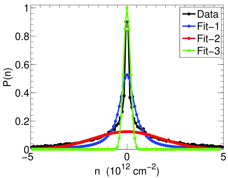
Figure 2: (Color online). Density probability distribution at the Dirac point for $n_{imp}=7.5\times 10^{13}$ cm^-2, $d=0.2$ nm and $\kappa=50$. The black line shows the TFDT result. The blue line is the fit $P=be^{-|n/a|}$ with $a=0.7\times 10^{12}$ cm^-2 and $b=0.5309$. The red line is the Gaussian fit to the tails of $P(n)$, $P=be^{-x^{2}/a^{2}}$ with $a=2.5\times 10^{12}$ cm^-2 and $b=.125$. The green line is the Gaussian fit to the center of $P(n)$, $P=be^{-x^{2}/a^{2}}$ with $a=0.25\times 10^{12}$ cm^-2 and $b=1.0.$

The knowledge of $P(n)$ allows the calculation of all the statistical properties that characterize the strongly inhomogeneous ground state of the surface of a 3DTI in the presence of disorder. The quantity that better quantifies the strength of the carrier density inhomogeneities is $n_{\rm rms}$, shown in Fig. 3 as a function of the average carrier density $\langle n\rangle$ for different values of $n_{\rm imp}$. As expected larger values of $n_{\rm imp}$ induce larger value of $n_{\rm rms}$. The interesting result is that $n_{\rm rms}$ also increases with $\langle n\rangle$ but the dimensionless ratio decreases with increasing average density. This is due to the fact that as $\langle n\rangle$ increases the range of values that $n$ can take locally also increases inducing larger values of $n_{\rm rms}$, but the dimensionless ratio of the density fluctuation to the average density decreases with increasing density.

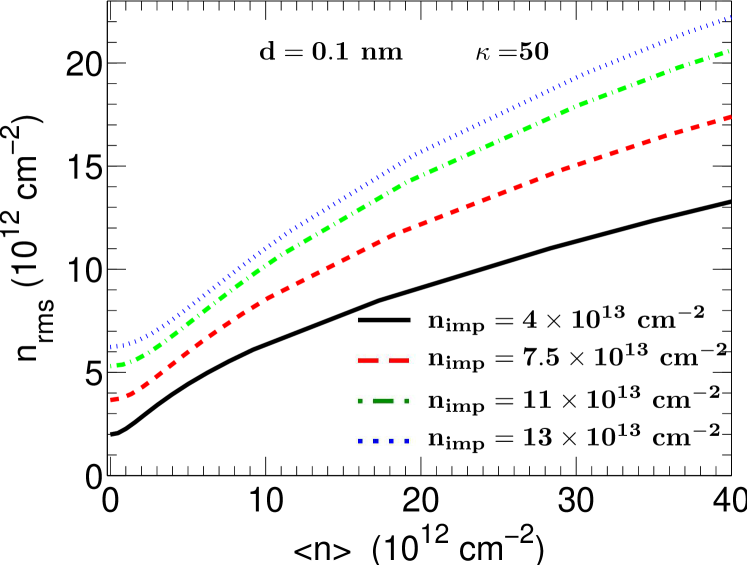
Figure 3: (Color online). Root mean square of the density fluctuations $n_{rms}$ as a function of the average density for different values of $n_{imp}$ with $d=0.1$ nm and $\kappa=50$.

Fig. 4 (a) shows the TFDT results for the root mean square of the screened disorder potential $s_{TFDT}$ as a function $\langle n\rangle$ for different values of $n_{\rm imp}$. As $\langle n\rangle$ increases the screening becomes more effective and therefore $s_{TFDT}$ decreases. However, we see that the dependence of $s_{TFDT}$ on $\langle n\rangle$ is fairly weak, for all values of $n_{\rm imp}$ considered. This fact justifies the assumption in the quasi-TFDT model to assume the variance of the effective distribution $P(V)$ to be independent of $\langle n\rangle$. Fig. 4 (b) shows the scaling of the ratio $s_{TFDT}/\sqrt{n_{imp}}$ versus $\langle n\rangle$. We can see that the ratio changes by less than 10% over a wide range of experimentally relevant values of the average density. This result is one more evidence of the weak dependence of $s_{TFDT}$ on $\langle n\rangle$—to the zeroth order, the inhomogeneity and fluctuations are determined by the impurity distribution $n_{imp}$ and $d$ (as well as the background dielectric constant $\kappa$).

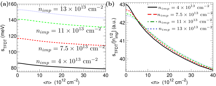
Figure 4: (Color online). (a) Root mean square of the screened disorder potential $s_{TFDT}$ as a function of average carrier density for different values of $n_{imp}$ with $d=0.1$ nm and $\kappa=50$ using TFDT. (b) $s_{TFDT}/\sqrt{n_{imp}}$ (in units of $\sqrt{10^{-13}}$meV$\cdot$cm) as a function of average carrier density.

The dependence of $n_{\rm rms}$ and $s_{TFDT}$ on $\kappa$ and $d$ is very strong as shown by Fig. 5 and Fig. 6. From Fig. 5 we see that both $n_{\rm rms}$ and $s_{TFDT}$ decrease rapidly as $\kappa$ increases. Increasing the average distance of the charged impurities from the surface of the 3DTI also strongly reduces the amplitude of the spatial inhomogeneities and therefore of $n_{\rm rms}$ and $s_{TFDT}$ as shown in Fig. 6.

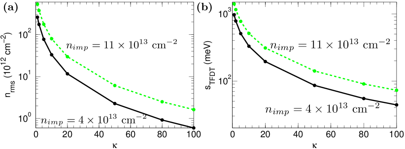
Figure 5: (Color online). TFDT results at the CNP for $d=0.1$ nm. (a) $n_{rms}$ as a function of substrate dielectric constant $\kappa$. (b) Root-mean-square of the screened disorder potential $s_{TFDT}$ as a function of substrate dielectric constant $\kappa$. The solid lines are for $n_{imp}=4\times 10^{13}$ cm^-2 and the dashed-lines are for $n_{imp}=11.0\times 10^{13}$ cm^-2.

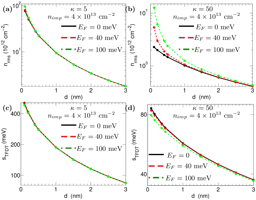
Figure 6: (Color online). (a) and (b) $n_{rms}$ at the Dirac point versus the distance $d$ of the charged impurity to the TI surface calculated within TFDT for $n_{imp}=4.0\times 10^{13}$ cm^-2. The solid, dashed and dot-dashed lines correspond to chemical potential $E_{F}=0$, $40$ and $100$ meV, respectively. (c) and (d) The corresponding $s_{TFDT}$ results versus $d$. (a) and (c) The effective background dielectric constant $\kappa=5$. (b) and (d) The effective background dielectric constant $\kappa=50$.

We now present a comparison of the TFDT results with the ones obtained using the self-consistent and the quasi-TFDT approaches, methods in which $P(V)$ is assumed to be Gaussian. Fig. 7 shows the scaling of the screened disorder rms obtained using the self-consistent approach ($s_{sc}$) versus doping and $\kappa$. These results, analogously to the TFDT results, show that $s$ depends very weakly on $\langle n\rangle$ and quite strongly on $\kappa$.

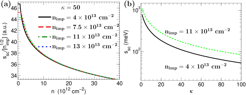
Figure 7: (Color online). Self-consistent results. (a) $s_{sc}/\sqrt{n_{imp}}$ (in units of $\sqrt{10^{-13}}$meV$\cdot$cm) as a function of carrier density for different values of $n_{imp}$ with $\kappa=50$ and $d=0.1$ nm. (b) Potential fluctuation $s_{sc}$ as a function of substrate dielectric constant $\kappa$. The solid lines are for $n_{imp}=4\times 10^{13}$ cm^-2 and the dashed-lines are for $n_{imp}=11.0\times 10^{13}$ cm^-2 with $d=0.1$ nm.

Fig. 8 shows the comparison for the value of $s$ at the CNP as a function of $d$ obtained using the three different methods: TFDT, quasi-TFDT and, self-consistent. We see that the self-consistent approach in general returns values of $s$ larger than the ones obtained using the TFDT. We should emphasize that $s$ obtained using the quasi-TFDT method is only an effective quantity that is used to calculate the transport properties within the 2-fluid model.

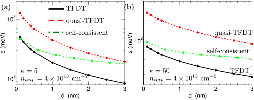
Figure 8: (Color online). Comparison of three methods for the potential fluctuation $s$ at the Dirac point versus the charged impurity distance $d$ to the TI surface for $n_{imp}=4.0\times 10^{13}$ cm^-2. The solid, dashed and dot-dashed lines correspond to the TFDT, quasi-TFDT and the self-consistent methods, respectively. (a) The effective background dielectric constant $\kappa=5$. (b) The effective background dielectric constant $\kappa=50$.

III.2 Transport at zero temperature

Using the TFDT and the EMT we can calculate the 2D conductivity on the surface of a 3DTI. Fig. 9 shows $\sigma$ as a function of doping, i.e. average density, for several values of $n_{\rm imp}$ and fixed $d=0.1$ nm and $\kappa=50$. As in graphene dassarma2011 the TFDT+EMT results recover the behavior of $\sigma(n)$ observed experimentally Dohun_arXiv11 : the linear scaling of $\sigma(n)$ at large doping, the finite value ($\sigma_{\rm min}$) of $\sigma$ for $n=0$, and the crossover regime for intermediate values of $n$. More importantly, the theory returns values of $\sigma_{\rm min}=(2-4)e^{2}/h$ (depending on the sample properties) that agree with the ones observed in experiments Dohun_arXiv11 .

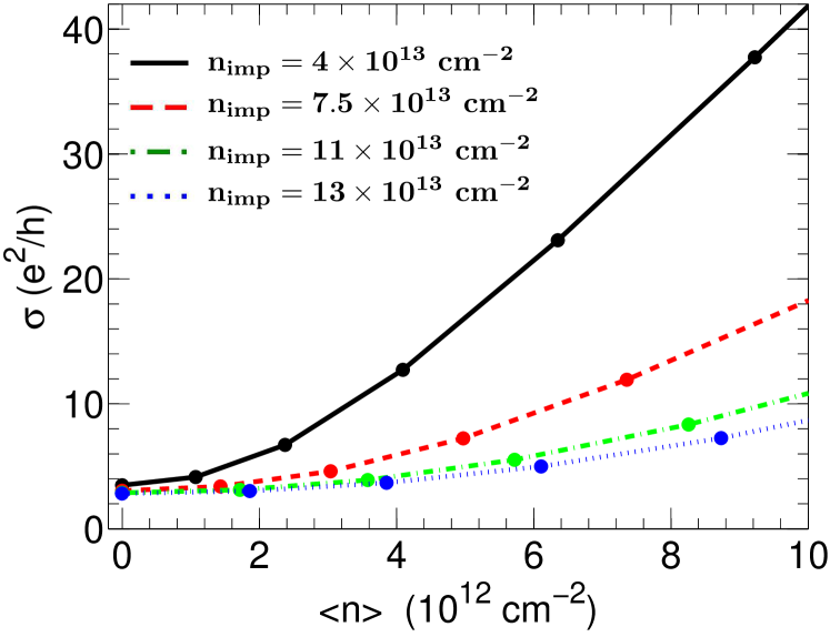
Figure 9: (Color online). TFDT-EMT conductivity as a function of average carrier density for different values of $n_{imp}$ with $d=0.1$ nm and $\kappa=50$.

Fig. 10 shows the comparison for the dependence of $\sigma$ with respect to $n$ obtained using the TFDT+EMT method and the 2-fluid approximations. From Fig. 10 we see that for $n_{\rm imp}\lesssim 4\times 10^{13}$ cm^-2 and values of $\kappa\gtrsim 50$, the three approaches give very similar results. For smaller values of $\kappa$ the three approaches give results that are qualitatively similar but that differ quantitatively. The general conclusion is that away from the CNP the three approaches agree quantitatively for samples with mobility $\mu>1000{\rm cm}^{2}/{\rm V\cdot s}$. For very low mobility highly-disordered TI systems (with 2D surface mobility lower than $1000$ cm²/V$\cdot$s even at $T=0$ ), we expect the TFDT to provide the most quantitatively accurate results. However, given that our main objective is to describe the universal qualities of the transport arising from the presence of inhomogeneities, and given the absence of accurate knowledge of the impurity distribution, i.e. $n_{imp}$ and $d$ in our model, for the purposes of this work the three approaches appear to be equivalent.

Figure 10: (Color online). Calculated conductivity as a function of carrier density for different values of the substrate dielectric constant with the impurity density $n_{imp}=4.0\times 10^{13}$ cm^-2 , $d=0.1$ nm. The solid, dashed and dot-dashed lines are obtained by using TFDT-EMT method, self-consistent method, and quasi-TFDT method, respectively.

Close to the CNP the three transport approaches give results that differ quantitatively as shown in Figs. 11-13. The self-consistent+2-fluid model for the parameter values relevant for TIs gives values of $\sigma_{\rm min}$ smaller than the ones obtained using the TFDT+EMT method. In TIs the agreement between the two methods close to the CNP is worse than in graphene Adam_SCC09 due to the fact that in TIs the density of charged impurities is larger than in typical graphene samples. It is remarkable to see how, in agreement with experiments, the three methods give that $\sigma_{\rm min}$ depends very weakly on $n_{\rm imp}$ and $\kappa$, for experimentally relevant parameter values. The weak dependence on $n_{\rm imp}$ can be qualitatively understood using the 2-fluid model result for $\sigma_{\rm min}$ Eq. (19) from which we see that $\sigma_{\rm min}$ is proportional to the ratio $s^{2}/n_{imp}$, and that on the other hand $s^{2}$ is proportional to $n_{\rm imp}$, Eq. (12). Within the semiclassical approach the very weak dependence of $\sigma_{\rm min}$ on $n_{\rm imp}$ and $\kappa$ is due to the fact that an increase (decrease) of $n_{\rm imp}$ ($\kappa$) increases the strength of the disorder potential that causes a decrease of the carriers mean free path $\ell$, and an increase of the amplitude of the carrier density inhomogeneities(i.e. the density of carriers in the electron-hole puddles). The reduction of $\ell$ and the increase of $n_{\rm rms}$ have opposite effect on $\sigma_{\rm min}$ and they almost cancel out jang2008 ; rossi2009 .

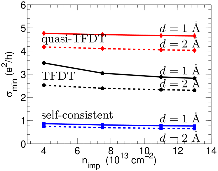
Figure 11: (Color online). The minimum conductivity $\sigma_{min}$ as a function of charged impurity density $n_{imp}$ with $\kappa=50$. The symbols diamond, circle and square denote the results obtained using the quasi-TFDT, TFDT-EMT and the self-consistent method, respectively. The solid and dashed lines correspond to the impurity distance $d=1$ Å and $d=2$ Å , respectively.

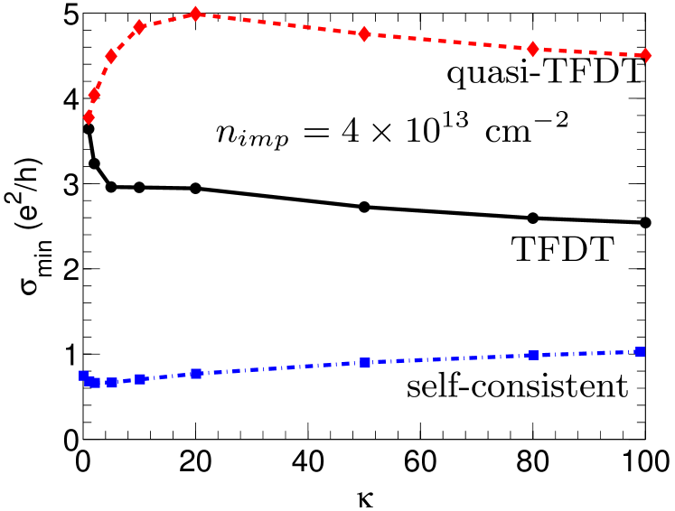
Figure 12: (Color online). The minimum conductivity $\sigma_{min}$ as a function background dielectric constant $\kappa$ for $n_{imp}=4.0\times 10^{13}$ cm^-2 , $d=0.1$ nm. The dashed, solid and dot-dashed lines denote the results obtained using the quasi-TFDT, TFDT-EMT and the self-consistent method, respectively.

The dependence of $\sigma_{\rm min}$ with respect to the average distance $d$ of the charged impurities from the TI’s surface is appreciably different for the three methods. The self-consistent+2-fluid model returns a very weak dependence of $\sigma_{\rm min}$ with respect to $d$. This is due to the weak dependence with respect to $d$ of $s^{2}$ obtained using the self-consistent approximation, Eq. (12). On the other hand the value of $s^{2}$ obtained using the TFDT is quite sensitive to the value of $d$ and as a consequence using the TFDT+EMT and the quasi-TFDT+2-fluid models we find that the dependence of $\sigma_{\rm min}$ on $d$ is not as weak as the one given from the self-consistent+2-fluid model. All the three approaches show that $\sigma_{\rm min}$ decreases as a function of $d$. This is due to the fact that as $d$ increases, due to the weakening of the disorder potential, the decrease of $n_{\rm rms}$ is faster than the increase of the mean free path.

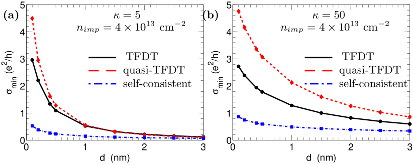
Figure 13: (Color online). The minimum conductivity $\sigma_{min}$ versus the charged impurity distance $d$ to the TI surface for $n_{imp}=4.0\times 10^{13}$ cm^-2. The solid, dashed and dot-dashed lines correspond to the TFDT-EMT, quasi-TFDT and the self-consistent methods, respectively. (a) The effective background dielectric constant $\kappa=5$. (b) The effective background dielectric constant $\kappa=50$.

III.3 Transport at finite temperature

In this section, using the 2-fluid model, we present our results for the conductivity in TIs at finite temperature. If we neglect the contribution of activation processes in TIs the dominant contribution to the temperature dependence of $\sigma$ is due to electron-phonon scattering processes. Fig. 14 shows the longitudinal acoustic phonon limited resistivity of Bi₂Se₃ surface as a function of temperature on a log-log plot. To calculate the Bi₂Se₃ surface resistivity due to phonon scatteringGiraud_PRB12 we use $D=30$ eV for the deformation potential coupling constant, $\rho_{m}\simeq 7.68\times 10^{-7}$ g/cm^-2 for the two dimensional mass density, i.e. 1 quintuple layer mass density of Bi₂Se₃, and $v_{l}=2900$ m/s is the velocity of the longitudinal acoustic phonon modeGiraud_PRB12 . The inset of Fig. 14 shows the logarithmic derivatives of the temperature-dependent resistivity. Fig. 14 clearly demonstrates two different regimes depending on whether the phonon system is degenerate or non-degenerate, and the low- to high-temperature crossover is characterized by the Bloch-Grüneisen (BG) temperature $T_{BG}=2k_{F}v_{l}/k_{B}$Hwang_phononPRB08 ; hongkihwang_PRB11 ; Giraud_PRB11 ; Giraud_PRB12 . The resistivity increases with $T$ as $\rho\sim T^{4}$ at low temperatures and $\rho\sim T$ at high temperatures, which agrees with the results obtained for TI films by using an isotropic elastic continuum approachGiraud_PRB12 . We note that electron-phonon scattering is an important scattering mechanism for finite-temperature transport in TIs, e.g., $T_{BG}\sim 30$ K in TIs compared to $T_{BG}\sim 100$ K in graphene because the latter has much larger phonon velocity. In graphene, in contrast to 2D surface TI transport, phonon effects are extremely weakHwang_phononPRB08 .

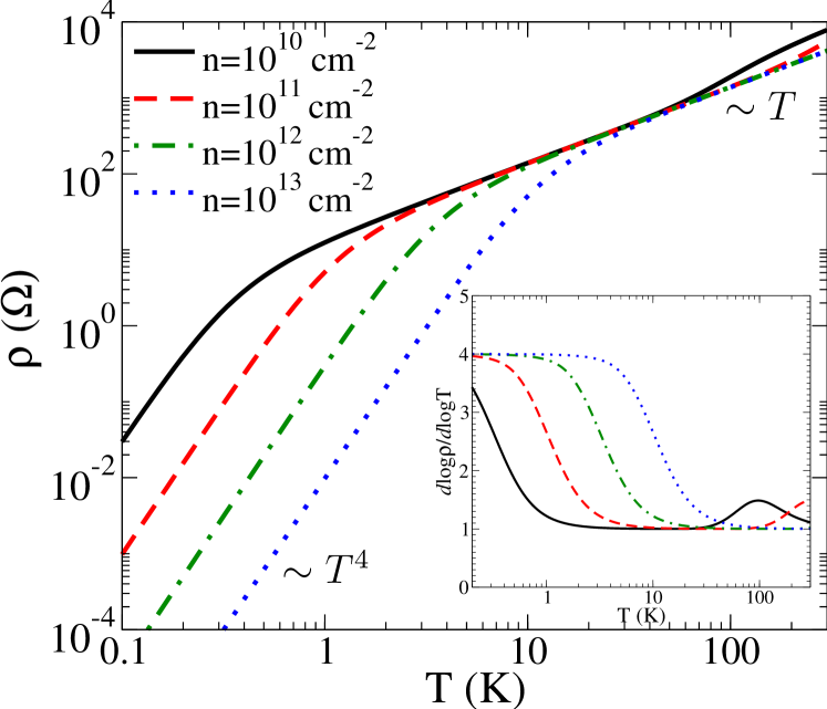
Figure 14: (Color online). Double-logarithmic scale of resistivity (Bi₂Se₃) only due to phonon scattering as a function of temperature for several densities. The deformation potential coupling constant $D=30$ eV, $\rho_{m}\simeq 7.68\times 10^{-7}$ g/cm^-2, and the velocity of longitudinal acoustic phonon mode $v_{l}=2900$ m/s. The inset shows the logarithmic derivatives $d\log\rho/d\log T$ versus temperature.

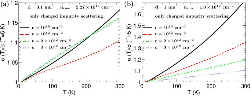
Figure 15: (Color online). Calculated conductivity as a function of temperature for different carrier density including only charged impurity scattering with $d=0.1$ nm, $\kappa=50$ and $n_{imp}=4\times 10^{13}$ cm^-2. (a) The charged impurity distance $d=0.1$ nm. The corresponding TFDT $n_{rms}\simeq 2.27\times 10^{12}$ cm^-2 and the potential fluctuation $s\simeq 220$ meV (Eq. 14). (b) The charged impurity distance $d=1$ nm. The corresponding TFDT $n_{rms}\simeq 1.0\times 10^{12}$ cm^-2 and the potential fluctuation $s\simeq 150$ meV (Eq. 14).

The results shown in Fig. 14 do not include the contribution to the resistivity due to quenched disorder. To include both the effect of quenched disorder and electron-phonon scattering we use the quasi-TFDT+2-fluid. As discussed in Sec. II, this approach allows us to take into account several finite temperature effects: the temperature dependence of the screening of the quenched disorder, electron-phonon scattering processes, broadening of the Fermi surface, and temperature induced activated processes. The temperature activated processes cause $\sigma$ to increase with $T$ and therefore induce an insulating behavior (i.e. conductivity increasing with increasing temperature) for $\sigma(T)$, whereas the electron-phonon scattering processes induce a metallic behavior (i.e. conductivity decreasing with increasing temperature). The change with $T$ of the screening of the disorder potential also induces a metallic behavior for $\sigma(T)$, however given the large value of $\kappa$ in typical TIs this effect is quite weak, contrary to the case of graphene dassarma2011 or 2D semiconductor systemsdassarma1999 . Figs. 15 (a), (b) show the dependence of $\sigma$ on $T$ obtained by neglecting the effect of electron-phonon scattering processes. We see that in this case the temperature dependence of $\sigma$ is almost completely determined by thermally activated processes that induce a monotonically increase of $\sigma$ with $T$.

Fig. 16 shows the scaling of the conductivity with respect to doping at different temperatures including both the effects of quenched disorder and electron-phonon scattering. At large densities the main effect of the finite temperature is to suppress $\sigma$ due to the presence of electron-phonon scattering processes. However, at low densities the effect of electron-phonon scattering processes competes with thermal activation processes and can give rise to a non-monotonic dependence of $\sigma$ with respect to $T$. This is shown in Figs. 17 (a), (b) where $\sigma(T)$ for different values of $n$ is plotted. From Figs. 17 (a), (b) we see that for $n\lesssim n_{\rm rms}$ at low temperatures the thermal activation processes dominate and induce an insulating behavior for $\sigma(T)$. The crossover temperature from insulating to metallic behavior depends on $n$, $n_{\rm imp}$, $\kappa$ and $d$. In general the larger the strength of the spatial fluctuations of the carrier density the stronger is the effect of thermal activation processes and therefore the larger is the low temperature range for which the transport exhibits insulating behavior. This is shown clearly by the scaling of $\sigma(T)$ at the CNP for different values of $n_{\rm imp}$, $\kappa$, Figs. 18 (a), (b), respectively. From Figs. 18 (a) and (b) we see that a change of $n_{\rm imp}$ and $\kappa$ that increases $n_{\rm rms}$ extends the range of temperatures over which $\sigma_{\rm min}(T)$ exhibit an insulating behavior.

The temperature dependence of $\sigma$ for different values of $d$ is shown in Fig. 18 (c). It appears to contradict the general rule that a parameter change that increases $n_{\rm rms}$ will increase the range of temperatures over which $\sigma(T)$ exhibit an insulating behavior. This is due to the combination of two effects: (i) The fact that at large $d$ ($d\gtrsim 1$ nm) $n_{\rm rms}$ is very low and so the resistivity $\rho_{dis}$ due to the quenched disorder at low carrier densities is much higher than the resistivity $\rho_{ph}$ due to electron-phonon scattering, so that $\sigma_{tot}(T)/\sigma_{tot}(T=5K)\approx\sigma_{dis}(T)/\sigma_{dis}(T=5K)$; (ii) The decrease at large $d$ of the metallic screening effects. The scaling of $\sigma$ with respect to $T$ and $d$ is therefore very interesting because it reveals the temperature dependence of the screening and could therefore be used to indirectly identify the nature of the disorder potential and the screening properties of the surfaces of 3DTIs.

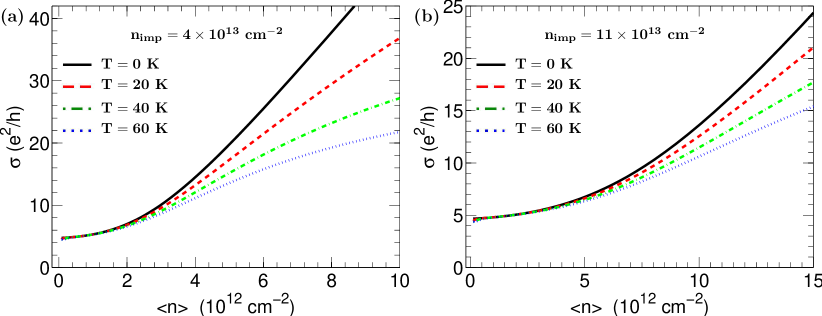
Figure 16: (Color online). Calculated conductivity as a function of net carrier density for various temperatures with $d=0.1$ nm and $\kappa=50$. (a) The impurity density $n_{imp}=4\times 10^{13}$ cm^-2. The corresponding TFDT $n_{rms}\simeq 2.27\times 10^{12}$ cm^-2 and the potential fluctuation $s\simeq 220$ meV (Eq. 14); (b) The impurity density $n_{imp}=11\times 10^{13}$ cm^-2. The corresponding TFDT $n_{rms}\simeq 4.21\times 10^{12}$ cm^-2 and the potential fluctuation $s\simeq 300$ meV (Eq. 14)

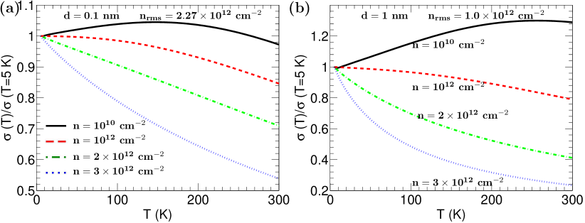
Figure 17: (Color online). Calculated conductivity as a function of temperature for different carrier density including both charged impurity and electron-phonon scattering, with $d=0.1$ nm, $\kappa=50$ and $n_{imp}=4\times 10^{13}$ cm^-2. (a) The charged impurity distance $d=0.1$ nm. The corresponding TFDT $n_{rms}\simeq 2.27\times 10^{12}$ cm^-2 and the potential fluctuation $s\simeq 220$ meV (Eq. 14). (b) The charged impurity distance $d=1$ nm. The corresponding TFDT $n_{rms}\simeq 1.0\times 10^{12}$ cm^-2 and the potential fluctuation $s\simeq 150$ meV (Eq. 14).

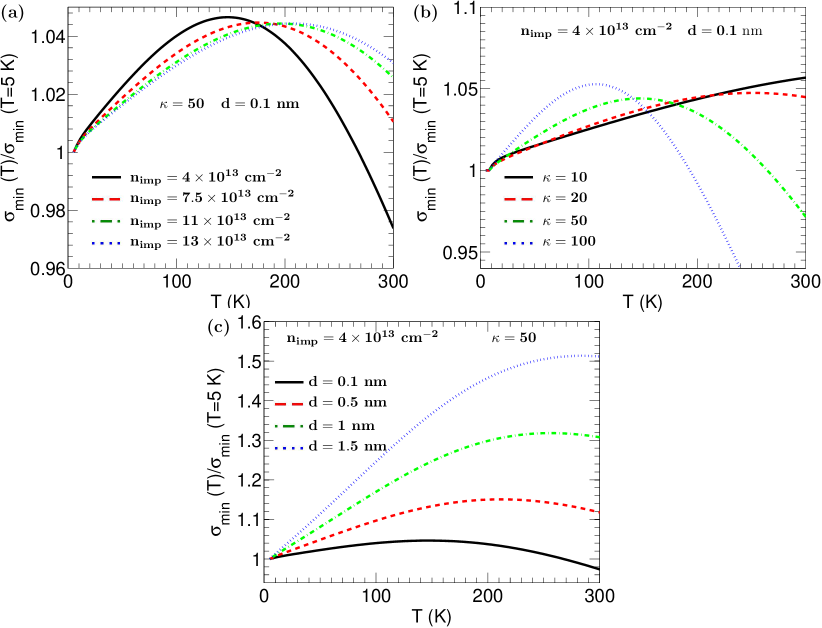
Figure 18: (Color online). Minimum conductivity as a function of temperature with (a) for various charged impurity density $n_{imp}$. As $n_{imp}$ increases, the corresponding $s=220,\ 300,\ 360,\ 390$ meV; (b) for various dielectric constant $\kappa$. As $\kappa$ increases, the corresponding $s=840,\ 500,\ 220,\ 110$ meV; (c) for various charged impurity distance $d$. As $d$ increases, the corresponding $s=220,\ 180,\ 150,\ 130$ meV. The corresponding potential fluctuation $s$ is obtained via Eq. 14 using $n_{rms}$ calculated within the TFDT (shown in Figs. 3, 5 and 6).

Before concluding this section on the temperature-dependent surface conductivity of 3DTIs, we point out that one of the important qualitative findings of our work is the nonmonotonic temperature dependence of the 2D surface conductivity as apparent in Figs. 16-18 and as expected from the competing mechanisms of phonon scattering and disorder induced density inhomogeneity. In particular, phonons induce higher-temperature metallic temperature dependence and the density inhomogeneity induces insulating temperature dependence through thermal activation, and at some disorder-dependent (and also doping-dependent) characteristic temperature the transport behavior changes from being insulating-like to metallic-like. We emphasize that this temperature-induced crossover behavior has nothing to do with any localization phenomenon (and in fact, Anderson localization effects are completely absent in TI surface transport since all back scattering is suppressed), and it arises entirely from a competition between inhomogeneity and phonons. The metallic behavior moves to higher (lower) temperature as disorder increases (decreases). This nonmonotonicity has been observed in experiments at lower 2D carrier densitieskim2012 where the inhomogeneity effects are important.

IV Conclusions

We have presented a detailed theoretical study of the 2D transport properties of the surfaces of 3DTIs. There is compelling evidence that in current transport experiments on 3DTIs charged impurities are the dominant source of quenched disorder. For this reason in our study we have considered in detail the case in which the quenched disorder potential is the one created by random charged impurities close to the surface of the TI. However, the theoretical framework that we have developed and presented in this work is very general. As in graphene, the presence of charged impurities induces the formation of strong carrier density inhomogeneities. In particular, close to the charge neutrality point the carrier density landscape breaks-up in electron-hole puddles. The strong carrier density inhomogeneities make the theoretical description of the electronic transport challenging for two reasons: (i) inability to use standard theoretical methods that assume a homogeneous density landscape; (ii) the importance at finite temperature of thermally activated processes. Our work presents a theoretical description of transport on the surface of 3DTIs that overcomes these difficulties and takes into account also the effect of electron-phonon scattering processes which is an important resistive mechanism at higher temperatures.

To characterize the disorder-induced inhomogeneities we use the Thomas-Fermi-Dirac-Theory. We also present a comparison of the results obtained using the TFDT with the one obtained using the self-consistent approximation and the quasi-TFDT approach and show that the three approaches give results that are qualitatively similar but that differ quantitatively.

To study the electronic transport in the presence of strong carrier density inhomogeneities, starting from the TFDT results, we use the effective medium theory and a 2-fluid model. The TFDT+EMT approach is well justified and is expected to provide the most accurate results. However, the generalization of the TFDT+EMT method to finite temperature is impractical due to the contribution to transport of thermally activated processes, contribution that can be dominant at low temperatures due to the strong carrier density inhomogeneities. At finite temperature the 2-fluid approach is very valuable because it allows to take into account all the finite temperature effects, such as temperature dependent screening and electron-phonon scattering, including thermally activated processes. The 2-fluid model relies on the use of an effective Gaussian distribution for the probability distribution of the screened potential $P(V)$. The parameters that define $P(V)$ can be chosen in such a way to maximize the agreement of the results for $T=0$ obtained using the 2-fluid model and the ones obtained using the TFDT+EMT approach. These parameters are then used to obtain the transport properties at finite temperature using the 2-fluid model.

In current 3DTIs the dielectric constant ($\kappa\sim 50$) is much larger than in graphene where $\kappa\sim 1-4$. In addition, in 3DTIs the acoustic phonon velocity is smaller than in graphene. These facts make the contribution of electron-phonon scattering processes to the resistivity much more important in the surface of 3DTIs than in graphene. For the surfaces of 3DTIs the effect of electron-phonon scattering events becomes important already for $T$ as low as 10 K, whereas in graphene it becomes relevant only for $T\gtrsim 200$ K. As a consequence for the surfaces of 3DTIs we find that electron-phonon scattering is much more important to determine the dependence of the conductivity on $T$. The large value of $\kappa$ in 3DTIs also implies that for the surface of 3DTIs, contrary to graphene, the temperature dependence of the screening does not play an important role. The temperature dependence of the conductivity on the surface of 3DTIs is therefore mostly determined by electron-phonon scattering processes and thermal activations processes. These two types of processes have opposite effect on $\sigma$ and at low temperature and low doping compete giving rise to a nonmonotonic dependence of $\sigma$ with respect to $T$. The nonmonotonic temperature dependence of the 2D surface conductivity is one of the important new qualitative results of our theory. We have presented detailed results for $\sigma(T)$ that clearly show the competition of the different processes that affect $\sigma$ for $T\neq 0$.

The theoretical approach developed here, being able to include all the main effects that determine the transport properties of the surfaces of 3DTIs, allowed us to present results that can be directly and quantitatively compared to the experimental ones. The good agreement between our theoretical results and the recent experimental measurements Dohun_arXiv11 ; Hong_arXiv11 ; Kong_Natnano ; Steinberg_PRB11 ; kim2012 , suggest that the theoretical method presented is very effective to characterize the transport properties of the surfaces of 3DTIs especially due to its ability to take into account the effects due to the disorder-induced carrier density inhomogeneities. Future improvement of the theory could include a more accurate surface band structure and the effects of the bulk bands, but we do not expect these details to affect our qualitative results at low surface doping densities because our theory includes the most important resistive processes contributing to the surface transport in 3DTIs.

- (1) M. Z. Hasan and C. L. Kane, Rev. Mod. Phys. 82, 3045 (2010)
- (2) L. Fu, C. L. Kane, and E. J. Mele, Phys. Rev. Lett. 98, 106803 (2007)
- (3) D. Culcer, Physica E 44, 860 (2012)
- (4) D. Hsieh, D. Qian, L. Wray, Y. Xia, Y. S. Hor, R. J. Cava, and M. Z. Hasan, Nature 452, 970 (2008)
- (5) Y. Xia, D. Qian, D. Hsieh, L.Wray, A. Pal, H. Lin, A. Bansil, D. Grauer, Y. S. Hor, R. J. Cava, and M. Z. Hasan, Nature Phys. 5, 398 (2009)
- (6) Y. Hsieh, D. Xia, D. Qian, L. Wray, J. H. Dil, F. Meier, J. Osterwalder, L. Patthey, J. G. Checkelsky, N. P. Ong, A. V. Fedorov, H. Lin, A. Bansil, D. Grauer, Y. S. Hor, R. J. Cava, and M. Z. Hasan, Nature 460, 1101 (2009)
- (7) Y. Chen, J. Analytis, J. Chu, Z. Liu, S. Mo, X. Qi, H. Zhang, D. Lu, X. Dai, Z. Fang, S.-C. Zhang, I. R. Fisher, Z. Hussain, and Z.-X. Shen, Science 325, 178 (2009)
- (8) D. Hsieh, Y. Xia, D. Qian, L. Wray, F. Meier, J. H. Dil, J. Osterwalder, L. Patthey, A. V. Fedorov, H. Lin, A. Bansil, D. Grauer, Y. S. Hor, R. J. Cava, and M. Z. Hasan, Phys. Rev. Lett. 103, 146401 (2009)
- (9) K. S. Novoselov, A. K. Geim, S. V. Morozov, D. Jiang, Y. Zhang, S. V. Dubonos, I. V. Grigorieva, and A. A. Firsov, Science 306, 666 (2004)
- (10) S. Das Sarma, S. Adam, E. H. Hwang, and E. Rossi, Rev. Mod. Phys. 83, 407 (2011)
- (11) N. P. Butch, K. Kirshenbaum, P. Syers, A. B. Sushkov, G. S. Jenkins, H. D. Drew, and J. Paglione, Phys. Rev. B 81, 241301 (2010)
- (12) D. Kim, S. Cho, N. P. Butch, P. Syers, K. Kirshenbaum, J. Paglione, and M. S. Fuhrer, Nature Phys. 8, 460 (2012)
- (13) S. S. Hong, J. J. Cha, D. Kong, and Y. Cui, Nat. Commun. 3, 757 (2012)
- (14) D. Kong, Y. Chen, J. J. Cha, Q. Zhang, J. G. Analytis, K. Lai, Z. Liu, S. S. Hong, K. J. Koski, S.-K. Mo, Z. Hussain, I. R. Fisher, Z.-X. Shen, and Y. Cui, Nat. Nano. 6, 705 (2011)
- (15) H. Steinberg, J.-B. Laloë, V. Fatemi, J. S. Moodera, and P. Jarillo-Herrero, Phys. Rev. B 84, 233101 (2011)
- (16) F. Wilczek, Phys. Rev. Lett. 58, 1799 (1987)
- (17) X.-L. Qi, T. L. Hughes, and S.-C. Zhang, Phys. Rev. B 78, 195424 (2008)
- (18) F. Wilczek, Nature 458, 129 (2009)
- (19) R. Li, J. Wang, X.-L. Qi, and S.-C. Zhang, Nat. Phys. 6, 284 (2010)
- (20) L. Fu and C. L. Kane, Phys. Rev. Lett. 100, 096407 (2008)
- (21) L. Fu and C. L. Kane, Phys. Rev. B 79, 161408 (2009)
- (22) J. E. Moore, Nature 464, 194 (2010)
- (23) M. Liu, C.-Z. Chang, Z. Zhang, Y. Zhang, W. Ruan, K. He, L.-l. Wang, X. Chen, J.-F. Jia, S.-C. Zhang, Q.-K. Xue, X. Ma, and Y. Wang, Phys. Rev. B 83, 165440 (2011)
- (24) D. Culcer, E. H. Hwang, T. D. Stanescu, and S. Das Sarma, Phys. Rev. B 82, 155457 (2010)
- (25) S. Adam, E. H. Hwang, and S. Das Sarma, Phys. Rev. B 85, 235413 (2012)
- (26) J. Martin, N. Akerman, G. Ulbricht, T.Lohmann, J. H. Smet, K. V. Klitzing, and A.Yacoby, Nat. Phys. 4, 144 (2008)
- (27) Y. Zhang, V. W. Brar, C. Girit, A. Zettl, and M. F. Crommie, Nat. Phys. 5, 722 (2009); A. Deshpande, W. Bao, F. Miao, C. N. Lau, and B. J. LeRoy, Phys. Rev. B 79, 205411 (2009); A. Deshpande, W. Bao, Z. Zhao, C. N. Lau, and B. J. LeRoy, Phys. Rev. B 83, 155409 (2011)
- (28) H. Beidenkopf, P. Roushan, J. Seo, L. Gorman, I. Drozdov, Y. S. Hor, R. J. Cava, and A. Yazdani, Nat. Phys. 7, 939 (2011)
- (29) E. Rossi and S. Das Sarma, Phys. Rev. Lett. 101, 166803 (2008)
- (30) R. C. Hatch, M. Bianchi, D. Guan, S. Bao, J. Mi, B. B. Iversen, L. Nilsson, L. Hornekær, and P. Hofmann, Phys. Rev. B 83, 241303 (2011)
- (31) E. H. Hwang and S. Das Sarma, Phys. Rev. B 75, 205418 (2007)
- (32) N. Kumar, B. A. Ruzicka, N. P. Butch, P. Syers, K. Kirshenbaum, J. Paglione, and H. Zhao, Phys. Rev. B 83, 235306 (2011)
- (33) W. Richter and C. R. Becker, Physica Status Solidi B 84, 619 (1977)
- (34) D. Kim, Q. Li, P. Syers, N. P. Butch, J. Paglione, S. D. Sarma, and M. S. Fuhrer, Phys. Rev. Lett. 109, 166801 (2012)
- (35) E. H. Hwang and S. Das Sarma, Phys. Rev. B 77, 115449 (2008)
- (36) S. Giraud and R. Egger, Phys. Rev. B 83, 245322 (2011)
- (37) S. Giraud, A. Kundu, and R. Egger, Phys. Rev. B 85, 035441 (2012)
- (38) C.-X. Liu, X.-L. Qi, H. Zhang, X. Dai, Z. Fang, and S.-C. Zhang, Phys. Rev. B 82, 045122 (2010)
- (39) M. Polini, A. Tomadin, R. Asgari, and A. MacDonald, Phys. Rev. B 78, 115426 (2008)
- (40) E. Rossi, S. Adam, and S. D. Sarma, Phys. Rev. B 79, 245423 (2009)
- (41) L. Brey and H. A. Fertig, Phys. Rev. B 80, 035406 (2009)
- (42) S. Das Sarma and E. H. Hwang, Phys. Rev. Lett. 102, 206412 (2009)
- (43) E. Rossi and S. Das Sarma, Phys. Rev. Lett. 107, 155502 (2011)
- (44) M. M. Fogler, D. S. Novikov, L. I. Glazman, and B. I. Shklovskii, Phys. Rev. B 77, 075420 (2008)
- (45) C. Beenakker, Rev. Mod. Phys. 80, 1337 (2008)
- (46) M. I. Katsnelson, K. S. Novoselov, and A. K. Geim, Nat. Phys. 2, 620 (2006)
- (47) A. V. Shytov, M. S. Rudner, and L. S. Levitov, Phys. Rev. Lett. 101, 156804 (2008)
- (48) N. Stander, B. Huard, and D. Goldhaber-Gordon, Phys. Rev. Lett. 102, 026807 (2009)
- (49) A. Young and P. Kim, Nature Physics 5, 222 (2009)
- (50) E. Rossi, J. H. Bardarson, P. W. Brouwer, and S. Das Sarma, Phys. Rev. B 81, 121408R (2010)
- (51) D. A. G. Bruggeman, Ann. Physik 416, 636 (1935)
- (52) R. Landauer, J. Appl. Phys. 23, 779 (1952)
- (53) M. Hori and F. Yonezawa, J. Math. Phys. 16, 352 (1975)
- (54) M. M. Fogler, Phys. Rev. Lett. 103, 236801 (2009)
- (55) E. Rossi, J. H. Bardarson, M. S. Fuhrer, and S. Das Sarma, Phys. Rev. Lett. 109, 096801 (2012)
- (56) Q. Li, E. H. Hwang, and S. Das Sarma, Phys. Rev. B 84, 115442 (2011)
- (57) S. Kirkpatrick, Rev. Mod. Phys. 45, 574 (1973)
- (58) E. H. Hwang and S. Das Sarma, Phys. Rev. B 82, 081409 (2010)
- (59) S. Adam, E. H. Hwang, V. M. Galitski, and S. Das Sarma, Proc. Natl. Acad. Sci. USA 104, 18392 (2007)
- (60) V. Galitski, S. Adam, and S. Das Sarma, Phys. Rev. B 76, 245405 (2007)
- (61) H. J. Zhang, C. X. Liu, X. L. Qi, X. Dai, Z. Fang, and S. C. Zhang, Nature Phys. 5, 438 (2009)
- (62) S. Adam, E. Hwang, E. Rossi, and S. Das Sarma, Solid State Communications 149, 1072 (2009)
- (63) C. Jang, S. Adam, J.-H. Chen, E. D. Williams, S. D. Sarma, and M. S. Fuhrer, Phys. Rev. Lett. 101, 146805 (2008)
- (64) H. Min, E. H. Hwang, and S. Das Sarma, Phys. Rev. B 83, 161404 (2011)
- (65) S. Das Sarma and E. H. Hwang, Phys. Rev. Lett. 83, 164 (1999)