Fast Converging Algorithm for Weighted Sum Rate Maximization in Multicell MISO Downlink

Abstract

The problem of maximizing weighted sum rates in the downlink of a multicell environment is of considerable interest. Unfortunately, this problem is known to be NP-hard. For the case of multi-antenna base stations and single antenna mobile terminals, we devise a low complexity, fast and provably convergent algorithm that locally optimizes the weighted sum rate in the downlink of the system. In particular, we derive an iterative second-order cone program formulation of the weighted sum rate maximization problem. The algorithm converges to a local optimum within a few iterations. Superior performance of the proposed approach is established by numerically comparing it to other known solutions.

I Introduction

For multiple-input multiple-output (MIMO) broadcast channels, dirty paper coding (DPC) is known to be the capacity-achieving scheme [1]. However, DPC is a nonlinear interference cancellation technique and thus requires high complexity. Hence, linear precoding techniques are of practical interest. Herein, we consider the problem of weighted sum rate maximization (WSRM) with linear transmit precoding for multicell multiple-input single-output (MISO) downlink. Unfortunately, the WSRM problem, even for single-antenna receivers as considered in this letter, has been shown to be NP-hard in [2]. Although optimal beamformers can be obtained using the methods presented, for instance, in [3, 4, 5], they may not be practically useful since the complexity of finding optimal designs grows exponentially with the problem size. Hence, the need of computationally conducive suboptimal solutions to the WSRM problem still remains.

Since the WSRM problem is nonconvex and NP-hard, there exists a class of beamformer designs which are based on achieving the necessary optimal conditions of the WSRM problem. In fact, this philosophy has been used, e.g., in [6, 7, 8, 9]. Interestingly, in [3], the authors have numerically shown that the suboptimal designs that achieve the necessary optimal conditions of the WSRM problem perform very close to the optimal design. In [6], the iterative coordinated beamforming algorithm was proposed by manipulating the Karush–Kuhn–Tucker (KKT) equations. However, this algorithm is not provably convergent. In [8, 9], the WSRM problem with joint transceiver design is solved using alternating optimization between transmit and receive beamforming. As we show by numerical results, these methods have a slower convergence rate compared to our proposed design.

In this letter, we propose a fast converging algorithm that locally solves the problem of WSRM for multicell MISO downlink. The idea of our iterative beamformer design is based on the framework of successive convex approximation (SCA) presented in [10]. The numerical results show that the proposed algorithm converges within a few iterations to a locally optimal point of the WSRM problem. The general concept of the SCA method is as follows. In each step of an iterative procedure, we approximate the original nonconvex problem by an efficiently solvable convex program and then update the variables involved until convergence. We note that in the context of transmit linear precoding for multicell downlink, the SCA method has been used, for example, in [7]. Basically, this method is based on convex relaxations of the rate function and generally arrives at more complex formulations. By proper transformations, we approximate the WSRM problem as a second-order cone program (SOCP) in each step of the SCA method. Our numerical results show that the proposed algorithm generally performs better than the known approaches, in particular, in terms of convergence rate.

Notation: We use standard notations in this letter. Bold lower and upper case letters represent vectors and matrices, respectively; $(.)^{\mbox{\scriptsize T}}$ represents the transpose operator. $\mathbb{C}^{a\times b}$ represents the space of complex matrices of dimensions given as superscripts; $|c|$ represents the absolute value of a complex number. Finally, $\|.\|_{2}$ represents the $l_{2}$ norm.

II Problem Formulation

Consider a system of $B$ coordinated BSs of $N$ transmit antennas each and $K$ single-antenna receivers. The set of all $K$ users is denoted by $\mathcal{U}=\{1,\,2\,\ldots,K\}$. We assume that data for the $k$th user is transmitted only from one BS, which is denoted by $b_{k}\in\mathcal{B}$, where $\mathcal{B}\triangleq\{1,2,\ldots,B\}$ is the set of all BSs. The set of all users served by BS $b$ is denoted by $\mathcal{U}_{b}$. Under flat fading channel conditions, the signal received by the $k$th user is

$$y_{k}=\mathbf{h}_{b_{k},k}\mathbf{w}_{k}d_{k}+\sum\limits_{i=1,i\neq k}^{K}\mathbf{h}_{b_{i},k}\mathbf{w}_{i}d_{i}+n_{k}$$ (1)

where $\mathbf{h}_{b_{i},k}\in\mathbb{C}^{1\times N}$ is the channel (row) vector from BS $b_{i}$ to user $k$, $\mathbf{w}_{k}\in\mathbb{C}^{N\times 1}$ is the beamforming vector (beamformer) from BS $b_{k}$ to user $k$, $d_{k}$ is the normalized complex data symbol, and $n_{k}\sim\mathcal{C}\mathcal{N}(0,\sigma^{2})$ is complex circularly symmetric zero mean Gaussian noise with variance $\sigma^{2}$. The term $\sum_{i=1,i\neq k}^{K}\mathbf{h}_{b_{i},k}\mathbf{w}_{i}d_{i}$ in (1) includes both intra- and inter-cell interference. The total power transmitted by BS $b$ is $\sum_{k\in\mathcal{U}_{b}}\bigl{\|}\mathbf{w}_{k}\bigr{\|}_{2}^{2}$. The SINR $\gamma_{k}$ of user $k$ is

$$\gamma_{k}=\frac{\bigl{|}\mathbf{h}_{b_{k},k}\mathbf{w}_{k}\bigr{|}^{2}}{\sigma^{2}+\sum_{i=1,i\neq k}^{K}\bigl{|}\mathbf{h}_{b_{i},k}\mathbf{w}_{i}\bigr{|}^{2}}.$$ (2)

In this letter, we are interested in the problem of WSRM under per-BS power constraints, which is formulated as

$$\begin{array}[]{rl}\underset{\mathbf{w}_{k}}{\operatorname*{maximize}}&\sum_{k=1}^{{}^{K}}\alpha_{k}\log_{2}(1+\gamma_{k})\\ \operatorname*{subject~{}to}&\sum_{k\in\mathcal{U}_{b}}\|\mathbf{w}_{k}\|_{2}^{2}\leq P_{b},\;\forall b\in\mathcal{B}\end{array}$$ (3)

where $\alpha_{k}$’s are positive weighting factors which are typically introduced to maintain a certain degree of fairness among users. As mentioned earlier, since problem (3) is NP-hard, the globally optimal design mainly plays as a theoretical benchmark rather than a practical solution [4]. Herein, we propose a low-complexity algorithm that solves (3) locally, i.e, satisfies the necessary optimal conditions of (3).

III Proposed Low-complexity Beamformer Design

To arrive at a tractable solution, we note that following monotonicity of logarithmic function, (3) is equivalent to

$$\begin{array}[]{rl}\underset{\mathbf{w}_{k}}{\operatorname*{maximize}}&\prod_{k}(1+\gamma_{k})^{\alpha_{k}}\\ \operatorname*{subject~{}to}&\sum_{k\in\mathcal{U}_{b}}\|\mathbf{w}_{k}\|_{2}^{2}\leq P_{b},\;\forall b\in\mathcal{B}\end{array}$$ (4)

which can be equivalently recast as

$$]{rl}\underset{{\mathbf{w}}_{k},t_{k}}{\operatorname*{maximize}} \quad\prod_{k}t_{k}$$ (5a)

$$\operatorname*{subject~{}to} \quad\gamma_{k}\geq t^{1/\alpha_{k}}_{k}-1,\;\forall k\in\mathcal{U}$$ (6a)

$$\quad\sum_{k\in\mathcal{U}_{b}}\|{\mathbf{w}}_{k}\|_{2}^{2}\leq P_{b},\;\forall b\in\mathcal{B}.$$ (7a)

The equivalence of (4) and (5a) can be easily recognized by noting the fact that all constraints in (6a) are active at the optimum. Otherwise, we can obtain a strictly larger objective by increasing $t_{k}$ without violating the constraints. Next, by introducing additional slack variables $\beta_{k}$, we can reformulate (5a) as

$$]{rl}\textstyle\underset{{\mathbf{w}}_{k},t_{k},\beta_{k}}{\operatorname*{maximize}} \quad\prod_{k}t_{k},$$ (8a)

$$\operatorname*{subject~{}to} \quad{\mathbf{h}_{b_{k},k}{\mathbf{w}}_{k}}\geq\sqrt{t^{1/\alpha_{k}}_{k}-1}\beta_{k},\forall k\in\mathcal{U},$$ (9a)

$$\quad\mathrm{Im}{({\mathbf{h}}_{b_{k},k}{\mathbf{w}}_{k})}=0,\forall k\in\mathcal{U},$$ (10a)

$$\quad\Bigl{(}{\sigma^{2}+\sum_{i\neq k}|{\mathbf{h}}_{b_{i},k}{\mathbf{w}}_{i}|^{2}\Bigr{)}^{1/2}\leq\beta_{k},\forall k\in\mathcal{U},}$$ (11a)

$$\quad\sum_{k\in\mathcal{U}_{b}}\|{\mathbf{w}}_{k}\|_{2}^{2}\leq P_{b},\;\forall b\in\mathcal{B}.$$ (12a)

The equivalence between (5a) and (8a) is justified as follows. First, we note that forcing the imaginary part of $\mathbf{h}_{b_{k},k}\mathbf{w}_{k}$ to zero in (10a) does not affect the optimality of (5a) since a phase rotation on $\mathbf{w}_{k}$ will result in the same objective while satisfying all constraints. Second, we can show that all the constraints in (11a) hold with equality at the optimum. Suppose, to the contrary, the constraint for some $k$ in (11a) is inactive. Let us define $\tilde{\beta}_{k}\triangleq\beta_{k}/\eta$ and $\tilde{t}_{k}\triangleq\{\eta^{2}(t_{k}^{1/\alpha_{k}}-1)+1\}^{\alpha_{k}}$, where $\eta$ is a positive scaling factor. Since the constraint (11a) is inactive, we can choose $\eta>1$ such that the constraints in (9a) and (11a) are still met if we replace $(\beta_{k},t_{k})$ by $(\tilde{\beta}_{k},\tilde{t}_{k})$. However, such a substitution results in a strictly larger objective because $\tilde{t}_{k}>t_{k}$ for $\eta>1$. This contradicts the fact that we have obtained an optimal solution.

As a step toward a low-complexity solution to the WSRM problem, we rewrite the constraint (9a) as

$$\mathbf{h}_{b_{k},k}\mathbf{w}_{k} \geq \sqrt{x_{k}}\beta_{k},\;\forall k\in\mathcal{U}$$ (13a)

$$x_{k}+1 \geq t^{1/\alpha_{k}}_{k},\;\forall k\in\mathcal{U}.$$ (14a)

Again, we can easily see that by replacing (9a) with (13a) and (14a), we obtain an equivalent formulation of (8a). The reason of doing so becomes clear shortly. Let us define $f(x_{k},\beta_{k})=\sqrt{x_{k}}\beta_{k}$ for $x_{k},\beta_{k}\geq 0$ and focus on the constraint (13a) first. Note that $f(x_{k},\beta_{k})$ is nonconvex on the defined domain, and thus (13a) is not a convex constraint. To deal with nonconvex constraints, we invoke a result of [10] which shows that if we replace $f(x_{k},\beta_{k})$ by its convex upper bound and iteratively solve the resulting problem by judiciously updating the variables until convergence, we can obtain a KKT point of (8a). To this end, for a given $\phi_{k}$ for all $k$, we define the function [10]

$$G(x_{k},\beta_{k},\phi_{k})\triangleq\tfrac{\phi_{k}}{2}\beta_{k}^{2}+\tfrac{1}{2\phi_{k}}x_{k}$$ (15)

which arises from the inequality of arithmetic and geometric means of $\phi_{k}\beta_{k}^{2}$ and $\phi_{k}^{-1}{x_{k}}$. It is easy to check that $G(x_{k},\beta_{k},\phi_{k})$ is a convex overestimate of $f(x_{k},\beta_{k})$ for a fixed $\phi_{k}>0$, i.e., $G(x_{k},\beta_{k},\phi_{k})\geq f(x_{k},\beta_{k})$ for all $\phi_{k}>0$. Moreover, when $\phi_{k}=\tfrac{\sqrt{x_{k}}}{\beta_{k}}$, it is plain to observe

$$f(x_{k},\beta_{k}) = G(x_{k},\beta_{k},\phi_{k})$$ (16a)

$$\nabla f(x_{k},\beta_{k}) = \nabla G(x_{k},\beta_{k},\phi_{k})$$ (17a)

where $\nabla f$ is the gradient of $f$. Obviously if $f(x_{k},\beta_{k})$ is replaced by $G(x_{k},\beta_{k},\phi_{k})$, (13a) can be formulated as a second-order cone (SOC) constraint as we shown in (22a).

Now we turn our attention to (14a). Recall that $t_{k}^{1/\alpha_{k}}$ is convex if $0<\alpha_{k}\leq 1$ and concave if $\alpha_{k}>1$, and that the optimal solution of (3) stays the same if we multiply all $\alpha_{k}$’s by the same positive constant. Thus, we can force (14a) to be convex by scaling down $\alpha_{k}$’s in (3) such that $0<\alpha_{k}\leq 1$ for all $k$. However, in this case, the constraint $x_{k}+1\geq t_{k}^{1/\alpha_{k}}$ cannot be directly written as an SOC constraint for $\alpha_{k}\in\mathbb{R}_{++}$. As our goal is to arrive at an SOCP, we instead scale $\alpha_{k}$’s in (3) such that $\alpha_{k}>1$ for all $k$ and thus $t_{k}^{1/\alpha_{k}}$ becomes concave. Again, in the light of [10], we replace the right side of the inequality in (14a) by its upper bound, which now can be obtained by the first order approximation due to the concavity of $t_{k}^{1/\alpha_{k}}$. Precisely, we have

$$t_{k}^{\tfrac{1}{\alpha_{k}}}\leq{t_{k}^{(n)}}^{\tfrac{1}{\alpha_{k}}}+\tfrac{1}{\alpha_{k}}{t_{k}^{(n)}}^{\tfrac{1}{\alpha_{k}}-1}(t_{k}-t_{k}^{(n)})$$ (18)

where $t_{k}^{(n)}$ denotes the value of variable $t_{k}$ in the $n$th iteration (i.e., the iteration corresponding to Algorithm 1 described later). In fact, we have linearized $t_{k}^{1/\alpha_{k}}$ around the operating point $t_{k}^{(n)}$. With (18), (14a) now becomes a linear inequality. We note that the linear approximation in (18) is trivially shown to satisfy the conditions in (16a) and (17a) at $t_{k}^{(n)}$. A question naturally arises is whether the linear approximation in (18) affects the optimal sum rate. Interestingly, our numerical experiments show that the WSR obtained with the successive approximation with $\alpha_{k}>1$ is identical to that when (14a) is forced to be convex by having $0<\alpha_{k}<1$ in (3) for all $k$. In terms of complexity, the linear inequality in (18) is more preferable since it requires lower computational effort compared to the original nonlinear equality constraint in (14a).

Replacing the right sides of (13a) and (14a) by the upper bounds in (15) and (18), respectively, we can formulate (8a) as an SOCP by noting that the objective in (8a), i.e., the product of $t_{k}$’s admits an SOC representation [12, 11]. The main ingredient in arriving at the SOCP representation is the fact that the hyperbolic constraint $uv\geq z^{2}$ where $u\geq 0$, $v\geq 0$ is equivalent to $\|[2z\;\;(u-v)]^{\mbox{\scriptsize T}}\|_{2}\leq(u+v)$. Let us illustrate the SOCP formulation of (8a) for the special case $K=2^{q}$, where $q$ is some positive integer. By collecting two variables at a time and incorporating the additional hyperbolic constraint corresponding to them, we rewrite (8a) as the SOCP in (19a), shown on the top of the page,

$$]{rl}\underset{\mathbf{w}_{k},t_{k},x_{k},\beta_{k},z_{k}^{i}}{\operatorname*{maximize}} \quad z^{(0)}$$ (19a)

$$\operatorname*{subject~{}to} \quad\bigl{\|}\bigl{[}2z_{i}^{(N-1)}\quad(t_{2i-1}-t_{2i})\bigr{]}^{\mbox{\scriptsize T}}\bigr{\|}_{2}\leq(t_{2i-1}+t_{2i}),\quad i=1,\ldots,2^{N-1}$$

$$\quad\qquad\qquad\cdots\cdots$$

$$\quad\bigl{\|}\bigl{[}2z^{(0)}\quad(z_{1}^{(1)}-z_{2}^{(1)})\bigr{]}^{\mbox{\scriptsize T}}\bigr{\|}_{2}\leq(z_{1}^{(1)}+z_{2}^{(1)}),$$ (21a)

$$\quad\bigl{\|}\bigl{[}\tfrac{1}{2}\bigl{(}\mathbf{h}_{b_{k},k}\mathbf{w}_{k}-\tfrac{1}{2\phi_{k}^{(n)}}x_{k}-1\bigr{)}\quad\sqrt{\tfrac{\phi_{k}^{(n)}}{2}}\beta_{k}\bigr{]}^{\mbox{\scriptsize T}}\bigr{\|}_{2}\leq\tfrac{1}{2}\bigl{(}\mathbf{h}_{b_{k},k}\mathbf{w}_{k}-\tfrac{1}{2\phi_{k}^{(n)}}x_{k}+1\bigr{)},\forall k\in\mathcal{U}$$ (22a)

$$\quad{t_{k}^{(n)}}^{1/\alpha_{k}}+\frac{1}{\alpha_{k}}{t_{k}^{(n)}}^{1/\alpha_{k}-1}(t_{k}-t_{k}^{(n)})\leq x_{k}+1,\;\forall k\in\mathcal{U},$$ (23a)

$$\quad\bigl{\|}\bigl{[}\sigma\quad\mathbf{h}_{b_{1},k}\mathbf{w}_{1}\,\cdots\,\mathbf{h}_{b_{k-1},k}\mathbf{w}_{k-1}\quad\mathbf{h}_{b_{k+1},k}\mathbf{w}_{k+1}\,\cdots\,\mathbf{h}_{b_{K},k}\mathbf{w}_{K}\bigr{]}^{\mbox{\scriptsize T}}\bigr{\|}_{2}\leq\beta_{k},\;\forall k\in\mathcal{U},$$ (24a)

$$\quad\sum_{k\in\mathcal{U}_{b}}\|\mathbf{w}_{k}\|_{2}^{2}\leq P_{b},\;\forall b\in\mathcal{B}.$$ (25a)

where $\phi_{k}^{(n)}$ is the value of $\phi_{k}$ in the $n$th iteration. In the case of $K\neq 2^{q}$, we define additional $t_{j}=1$ for $j=K+1,\ldots,2^{\left\lceil\log_{2}K\right\rceil}$, where $\left\lceil x\right\rceil$ is the smallest integer not less than $x$ and the above expression still holds [11]. Now we are in a position to present an algorithm that solves problem (3) locally. The pseudocode of the beamformer design is outlined in Algorithm 1.

0:  $n=0$, $(\phi_{k}^{(n)},t_{k}^{(n)})=\textrm{random}$.

1:  repeat

2:     Solve (19a) with $\phi_{k}^{(n)}$ and $t_{k}^{(n)}$, and denote optimal $(t_{k},\beta_{k},x_{k})$ as $(t_{k}^{\star},\beta_{k}^{\star},x_{k}^{\star})$.

3:     Update $(t_{k}^{(n+1)},\beta_{k}^{(n+1)},x_{k}^{(n+1)})=(t_{k}^{\star},\beta_{k}^{\star},x_{k}^{\star})$ and $\phi_{k}^{(n+1)}=\frac{\sqrt{x_{k}^{(n+1)}}}{\beta_{k}^{(n+1)}}$; $n:=n+1$.

4:  until convergence

Algorithm 1 Proposed beamformer design for the WSRM problem in multicell MISO downlink.

We now present the convergence analysis of Algorithm 1. Consider the $n+1$st iteration of Algorithm 1 that solves the optimization problem (19a). If we replace $(t_{k},\beta_{k},x_{k})$ by $(t_{k}^{(n)},\beta_{k}^{(n)},x_{k}^{(n)})$ and $\mathbf{w}_{b,k}$ by $\mathbf{w}_{b,k}^{(n)}$, all the constraints in (22a)-(25a) are still satisfied. That is to say, the optimal solution of the $n$th iteration is a feasible point of the problem in the $n+1$st iteration. Thus, the objective obtained in the $n+1$st iteration is larger than or equal to that in the $n$th iteration. In other words, Algorithm 1 generates a nondecreasing sequence of objective values. Moreover, the problem is bounded above due to the power constraints. Hence, Algorithm 1 converges to some local optimum solution of (19a). By the two properties shown in (16a) and based on the arguments presented in [10], it can be shown that this solution also satisfies the KKT conditions of (8a). Numerical results in Section IV confirm that Algorithm 1 performs very close to optimal linear design.

IV Numerical Results

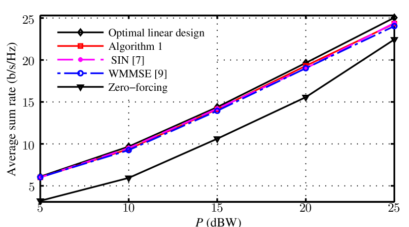
Figure 1: Average sum rate comparison for single-cell scenario, $N=4$, $K=4$.

In this section, we numerically evaluate the performance of Algorithm 1 under different setups using YALMIP [13] with SDPT3 [14] as internal solver. In the first experiment, we consider a single-cell scenario where a BS with $N=4$ transmit antennas serves $K=4$ users. The entries of $\mathbf{h}_{b,k}$ are $\mathcal{CN}(0,1)$ and the noise variance $\sigma^{2}=1$. In Fig. 1, we plot the average sum rate ($\alpha_{k}=1$ for all $k$) versus the total transmit power $P$ at the BS. The achieved sum rate of Algorithm 1 is compared to those of zero-forcing beamforming [15], the weighted sum mean-square error minimization (WMMSE) algorithm in [9], the soft inference nulling (SIN) scheme in [7], and the optimal linear design using the branch-and-bound (BB) method in [4, 3]. Initial values for beamformers for the suboptimal schemes in [9, 7], and $(\phi_{k}^{(0)},t_{k}^{(0)})$ in Algorithm 1 are generated randomly. The sum rate is obtained after Algorithm 1 and the iterative suboptimal schemes in [9, 7] converge, i.e., the increase in the objective value between two consecutive iterations is less then $10^{-2}$. The gap tolerance between the upper and lower bounds for the BB method is set to $10^{-1}$ as in [4, 3], and the resulting sum rate is calculated as the average of the upper and lower bounds. Results reveal that the average sum rate of Algorithm 1 and other iterative beamformer designs is the same on convergence and close to that of the optimal linear approach. However, the SIN scheme, WMMSE algorithm and the optimal design have a slower convergence rate as discussed next.

In the second experiment, we illustrate the convergence rate of all considered iterative suboptimal schemes. A simple two-cell scenario with each BS serving $2$ users is considered. The number of transmit antennas at each BS is set to $N=8$. The weights, without loss of generality, are taken as $(\alpha_{1},\alpha_{2},\alpha_{3},\alpha_{4})=(0.14,0.21,0.28,0.36)$ and the power budget of each BS is set to $P_{b}=12$ dB for $b=1,2$. Fig. 2 compares the weighted sum rate of the considered schemes as a function of iterations needed to obtain a stabilized output for a random channel realization. In particular, our algorithm has converged just after a few of iterations, while the WMMSE algorithm is still less than midway to convergence. In fact, for this particular case the WMMSE took hundreds of runs before converging to the local optimum solution. This observation may be attributed to the fact that optimization strategy of [9] requires alternate updates between transmit and receive beamformers and therefore exhibits slower convergence properties. We have also noticed that for certain initial values the convergence rate of the WMMSE algorithm is greatly improved. In fact, it was reported in [16] that the convergence rate of an alternating optimization algorithm depends on the initial values of the variables involved, and it converges quickly if initial guess is relatively close to the optimal solution. Further, we observe that Algorithm 1 with and without scaling has slightly different convergence rate (labeled in Fig. 2 as ‘approximated’ and ‘not approximated’) but same optimal value. This validates that the approximation used to arrive at an SOCP formulation has no impact on the achieved sum rate. Our numerical results reveal that for other channel realizations, the SIN scheme may have similar convergence behavior to Algorithm 1, but the average per iteration running time of Algorithm 1 is approximately four times less than that of the SIN method. For the set of channel realizations considered in Fig. 2, the optimal design also converges to the same point achieved by other iterative suboptimal methods. However, it takes more than $600$ iterations to reduce the gap between lower and upper bounds of the BB method to less than $10^{-1}$. Theoretically, the faster convergence of Algorithm 1 may be attributed to solving an explicit SOCP in each of its iterations. The faster convergence of our algorithm can be much useful for distributed implementation which is left as future work.

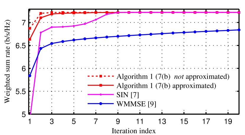
Figure 2: Convergence rate of the weighted sum rate, $B=2$, $N=8$, $K=4$, $P_{b}=12$ dB for all $b$.

V Conclusion

In the letter we have studied the problem of WSRM in the downlink of multicell MISO system. Since the problem is NP-hard, we have proposed a low-complexity approximation of the optimization problem. We show that the problem can be approximated by an iterative SOCP procedure. While the convergence of the algorithm can be proved, its global optimality cannot be established. Nonetheless, the algorithm outperforms the previously studied solutions to the WSRM problem, in particular, in terms of its convergence rate.

References

- [1] H. Weingarten, Y. Steinberg, and S. Shamai, “The capacity region of the Gaussian multiple-input multiple-output broadcast channel,” IEEE Trans. Inf. Theory, vol. 52, no. 9, pp. 3936–3964, Sep. 2006.
- [2] Z.-Q. Luo and S. Zhang, “Dynamic spectrum management: Complexity and duality,” IEEE J. Sel. Topics Signal Process., vol. 2, no. 1, pp. 57–73, Feb. 2008.
- [3] S. Joshi, P. Weeraddana, M. Codreanu, and M. Latva-aho, “Weighted sum-rate maximization for MISO downlink cellular networks via branch and bound,” IEEE Trans. Signal Process., vol. 60, no. 4, pp. 2090–2095, Apr. 2012.
- [4] E. Björnson, G. Zheng, M. Bengtsson, and B. Ottersten, “Robust monotonic optimization framework for multicell MISO systems,” IEEE Trans. Signal Process., vol. 60, no. 5, pp. 2508–2523, May 2012.
- [5] L. Liu, R. Zhang, and K.-C. Chua, “Achieving global optimality for weighted sum-rate maximization in the K-user Gaussian interference channel with multiple antennas,” IEEE Trans. Wireless Commun., vol. 11, no. 5, pp. 1933–1945, May 2012.
- [6] L. Venturino, N. Prasad, and X. Wang, “Coordinated linear beamforming in downlink multi-cell wireless networks,” IEEE Trans. Wireless Commun., vol. 9, no. 4, pp. 1451–1461, Apr. 2010.
- [7] Chris T. K. Ng and H. Huang, “Linear precoding in cooperative MIMO cellular networks with limited coordination clusters,” IEEE J. Sel. Areas Commun., vol. 28, no. 9, pp. 1446–1454, Dec. 2010.
- [8] S. S. Christensen, R. Agarwal, E. Carvaldho, and J. Cioffi, “Weighted sum-rate maximization using weighted MMSE for MIMO-BC beamforming design,” IEEE Trans. Wireless Commun., vol. 7, no. 12, pp. 4792–4799, Dec. 2008.
- [9] Q. Shi, M. Razaviyayn, Z.-Q. Luo, and C. He, “An iteratively weighted MMSE approach to distributed sum-utility maximization for a MIMO interfering broadcast channel,” IEEE Trans. Signal Process., vol. 59, no. 9, pp. 4331–4340, Sep. 2011.
- [10] A. Beck, A. Ben-Tal, and L. Tetruashvili, “A sequential parametric convex approximation method with applications to nonconvex truss topology design problems,” Journal of Global Optimization, vol. 47, no. 1, pp. 29–51, 2010.
- [11] F. Alizadeh and D. Goldfarb, “Second-order cone programming,” Mathematical Programming, vol. 95, pp. 3–51, 2001.
- [12] M. Lobo, L. Vandenberghe, S. Boyd, and H. Lebret, “Applications of second-order cone programming,” Linear Algebra and its Applications, vol. 248, pp. 193–228, Nov. 1998.
- [13] J. Löfberg, “YALMIP : A toolbox for modeling and optimization in MATLAB,” in Proc. the CACSD Conference, Taipei, Taiwan., 2004. [Online]. Available: http://users.isy.liu.se/johanl/yalmip
- [14] K. C. Toh, M. J. Todd, and R. Tutuncu, “SDPT3— a Matlab software package for semidefinite programming,” Optimization Methods and Software, Nov. 1999.
- [15] Q. Spencer, A. Swindlehurst, and M. Haardt, “Zero-forcing methods for downlink spatial multiplexing in multiuser MIMO channels,” IEEE Trans. Signal Process., vol. 52, no. 2, pp. 461–471, Feb. 2004.
- [16] J. C. Bezdek and R. J. Hathaway, “Convergence of alternating optimization,” Neural, Parallel and Scientific Computations, vol. 11, no. 4, pp. 351–368, Dec. 2003.