On the Survivability and Metamorphism of Tidally Disrupted Giant Planets: the Role of Dense Cores

Abstract

A large population of planetary candidates in short-period orbits have been found recently through transit searches, mostly with the Kepler mission. Radial velocity surveys have also revealed several Jupiter-mass planets with highly eccentric orbits. Measurements of the Rossiter-McLaughlin effect indicate that the orbital angular momentum vector of some planets is inclined relative to the spin axis of their host stars. This diversity could be induced by post-formation dynamical processes such as planet-planet scattering, the Kozai effect, or secular chaos which brings planets to the vicinity of their host stars. In this work, we propose a novel mechanism to form close-in super-Earths and Neptune-like planets through the tidal disruption of gas giant planets as a consequence of these dynamical processes. We model the core-envelope structure of gas giant planets with composite polytropes which characterize the distinct chemical composition of the core and envelope. Using three-dimensional hydrodynamical simulations of close encounters between Jupiter-like planets and their host stars, we find that the presence of a core with a mass more than ten times that of the Earth can significantly increase the fraction of envelope which remains bound to it. After the encounter, planets with cores are more likely to be retained by their host stars in contrast with previous studies which suggested that coreless planets are often ejected. As a substantial fraction of their gaseous envelopes is preferentially lost while the dense incompressible cores retain most of their original mass, the resulting metallicity of the surviving planets is increased. Our results suggest that some gas giant planets can be effectively transformed into either super-Earths or Neptune-like planets after multiple close stellar passages. Finally, we analyze the orbits and structure of known planets and Kepler candidates and find that our model is capable of producing some of the shortest-period objects.

1. Introduction

In contrast to the kinematic architecture of our solar system, there is a population of recently discovered exoplanets or planetary candidates that have orbital periods ranging from days to weeks. Depending on their masses, these close-in planets are commonly referred to as hot Jupiters or super Neptunes. Their relative abundance in the period distribution comes as the result of observational bias as the current radial velocity and transit surveys are more well suited for their detection than the identification of planets with longer period and lower masses. Recently, the Kepler mission has extended the detection limit down to sub-Earth size objects, and unveiled a rich population of close-in super-Earth and sub-Neptune candidates (defined in terms of their sizes) around solar type stars (Batalha et al., 2012).

The origin of these close-in planets remains poorly understood. A widely adopted scenario is based on the assumption that all gas giant planets formed beyond the snow line a few AU from their host star (Pollack et al., 1996), with the progenitors of hot Jupiters undergoing substantial inward migration through planet-disk interaction (see, e.g., Lin et al., 1996; Ida & Lin, 2004; Papaloizou & Terquem, 2006). This mechanism naturally leads to the formation of resonant gas giants (Lee & Peale, 2002) and coplanarity between the planets’ orbits and their natal disks. However, measurements of the Rossiter-McLaughlin effect (Ohta et al., 2005) reveal that the orbits of a sub population of hot Jupiters (around relatively massive and hot main sequence stars) appear to be misaligned with the spin of their host stars (Winn et al., 2010; Schlaufman, 2010). As the stellar spin is assumed to be aligned with that of their surrounding disks (Lai et al., 2011), the observed stellar spin-planetary orbit obliquity poses a challenge to the disk-migration scenario for the origin of hot Jupiters (Triaud et al., 2010; Winn et al., 2011).

In order to reconcile the theoretical predictions with the observations, some dynamical processes have been proposed, such as the Kozai mechanism (Kozai, 1962; Takeda & Rasio, 2005; Matsumura et al., 2010; Naoz et al., 2011; Nagasawa & Ida, 2011), planet-planet scattering (Rasio & Ford, 1996; Chatterjee et al., 2008; Ford & Rasio, 2008) or secular chaos (Wu & Lithwick, 2011), all of which operate after the gas is depleted and the onset of dynamical instability can produce highly eccentric orbits and considerably large orbital obliquity. The observed eccentricity distribution of extra-solar planets with periods longer than a week and masses larger than that of Saturn has a median value noticeably deviated from zero. Presumably they obtained this eccentricity through dynamical instability after the depletion of their natal disks (Lin & Ida, 1997; Zhou et al., 2007; Chatterjee et al., 2008; Jurić & Tremaine, 2008), as the eccentricity damping would suppress such an instability if they were embedded in a gaseous disk environment.

Some of these processes can produce planets that lie on nearly parabolic orbits. As their eccentricity approaches unity, planets with a semimajor axis of a few AU undergo close encounters with their host stars. At their pericenters, tides raised by the host star dissipate orbital energy into the planet’s internal energy, resulting in the shrinkage of their semimajor axes. The repeated subsequent encounters may lead to the circularization of their orbits (Press & Teukolsky, 1977), and provided there is no mass loss, the planet’s long-term orbital evolution may be modeled analytically (Ivanov & Papaloizou, 2007). However, when giant planets approach their host stars within several stellar radii, the tidal force may become sufficiently intense that it can lead to mass loss or tidal distruption. One particular example is WASP-12b (Li et al., 2010), which is being tidally distorted and is continuously losing its mass.

Hydrodynamical simulations have been carried out by Faber et al. (2005, hereafter FRW) and Guillochon et al. (2011, hereafter GRL) to study the survivability and orbital evolution of a Jupiter-mass planet disrupted by a Sun-like star. In the description of the relative strength of the tidal field exerted on a planet by the host star, it is useful to define a characteristic tidal radius as

$$r_{\rm t}\equiv\left(\frac{M_{*}}{M_{\rm P}}\right)^{1/3}R_{\rm P},$$ (1)

where $M_{\rm P}$ and $R_{\rm P}$ are the planetary mass and radius, and $M_{*}$ is the stellar mass (not to be confused with the Hill radius and Roche radius, which in this context commonly refer to a separation distance as measured from the the center of mass of the secondary). At this separation, the volume-averaged stellar density equals to the planetary mean density, i.e. $r_{\rm t}\simeq 1\ R_{\odot}$ in this case. Our previous simulations of single nearly parabolic (with $e\simeq 1$) encounters show the existence of a mass-shedding region demarcated by $r_{\rm p}/r_{\rm t}\lesssim 2$, where $r_{\rm p}$ is periastron distance. The planet’s specific orbital binding energy after the (either parabolic or highly elliptical) encounters is smaller for larger impact parameters ($\beta=r_{\rm t}/r_{\rm p}$), despite an enhanced stellar tidal perturbation. Within a sufficiently close range, planets are ejected due to mass and energy loss near periastron.

For the more distant periastron encounters, we also investigated planet’s response after multiple passages (see GRL, Section 3.2). We considered orbits with $e=0.9$ and $r_{\rm p}/r_{\rm t}\gtrsim 2$ and showed that successive encounters can enhance planetary mass and energy changes. We found a critical periastron separation $r_{\rm p}=2.7\ r_{\rm t}$ within which no planet can avoid destruction. However, this critical value only places a lower limit on non-destructive tidal interactions, as the accumulation of energy required to destroy a planet at wider separations occurs over a much longer time scale, which has not yet been investigated. We also noted that the semimajor axes of several known exoplanets are less than twice this critical separation. If they were scattered to the proximity of the star on a highly eccentric orbit ($e\gtrsim 0.9$), the initial periastron separation would be less than $2.7\ r_{\rm t}$, and thus they would have already been destroyed. We suggested that either these planets were scattered from a distance that is substantially closer to the host star than the snow line, or they were scattered to a further separation and then later migrated inward under the influence of tidal interaction with their host stars to their present positions.

To summarize, the observed inner edge of hot Jupiters seems to suggest they were tidally circularized (Ford & Rasio, 2006; Hellier et al., 2012), as the hydrodynamical simulations (FRW and GRL) showed that tidal dissipation within the planet alone either results in the planet’s ejection or disruption. In this work, we re-examine the disruption and retention of gas giant planets during their close encounters with their host stars by taking into account the presence of their dense cores. This possibility is not only consistent with the internal structure of Saturn (and to a much less certain extent in Jupiter, Guillot et al., 2004), but is also consistent with the widely adopted core accretion scenario (Pollack et al., 1996). We show that presence of a core with mass as small as $10\ M_{\earth}$, e.g. 3% of a Jupiter-like planet’s total mass, the planet has a far greater chance of survival, even with a mass loss comparable to the mass within its own envelope. We also consider the possibility that the tidal disruption mechanism may be an efficient way to transform a Jupiter-mass planet into a close-in super-Earth or Neptune-like object, which potentially may explain the existence of some of the inner edge of close-in planets.

Our paper is organized as follows. In Section 2, we introduce a composite polytrope model for planets with cores. Our setup for hydrodynamic simulations is described in Section 3.1. We present our simulation results in Section 3.2. In Section 4, we first discuss the adiabatic responses of mass-losing composite polytropes and explain the enhanced survivability of planets with cores as suggested by our numerical results, and search for potential candidates of tidally disrupted planets in the current exoplanet sample (including Kepler candidates). We summarize our work and probe the future directions in Section 5.

2. A Composite Polytrope Model for Gas Giant Planets with Cores

The core-envelope structure of gas giant planets is determined by the equation of state (EOS), their metal content, and their thermal evolution (Guillot et al., 2004). For computational simplicity, we approximate this structure by a composite polytrope model. This class of models is thoroughly described in Horedt (2004). Previously, a set of composite $n_{1}=3$ and $n_{2}=1.5$ polytropes has been used to represent the radiative core and the convective envelope of stars (Rappaport et al., 1983). By finding the intersection of the solutions of the Lane-Emden equation in the core and envelope on the U-V plane (see e.g. chapter 21 of Kippenhahn & Weigert, 1994), the overall physical properties envelope in stars can be calculated. In this paper, we adopt this approach with the incorporation of different species to model the transition in the composition and EOS at the core-envelope interface in giant planets (see Figure 1).

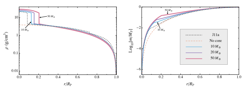
Figure 1.— One-dimensional profiles of density (left) and enclosed mass (right) of a composite polytropic model ($n_{1}=0.5$ and $n_{2}=1$) for a Jupiter-mass planet with no core, a $10M_{\oplus}$ core, a $20M_{\oplus}$ core, and a $50M_{\oplus}$ core. Note the density jump (left panel) and the discontinuity of the derivative of mass distribution (right panel) at the core-envelope interfaces are a result of the difference in molecular weight between the two zones, $\mu_{1}=4\mu_{2}$. The single $n=1$ polytropic model (dashed line) used in our previous simulations together with a profile of Jupiter with a 2.75 $M_{\oplus}$ core (dotted line) taken from Nettelmann et al. (2008) are plotted for comparison.

The polytropic approximation is simple to use because the pressure $P$ is a power-law function of the density $\rho$ only

$$P=K\rho^{\gamma}=K\rho^{(n+1)/n},$$ (2)

where $K$ is a constant. We denote the quantities related to the core and envelope by subscripts 1 and 2, respectively. To model the composite polytropic planet, we choose the polytropic indices to be $n_{1}=0.5$ and $n_{2}=1$ in the core and envelope, corresponding to $\gamma_{1}=3$ and $\gamma_{2}=2$.

Following Rappaport et al. (1983), we express the densities and pressures as

$$\rho_{1}=\rho_{\rm 1c}\theta_{1}^{n_{1}},\;P_{1}=K_{1}\rho_{\rm 1c}^{(n_{1}+1)/n_{1}}\theta_{1}^{n_{1}+1},$$ (3)

$$\rho_{2}=\rho_{\rm 2i}\theta_{2}^{n_{2}},\;P_{2}=K_{2}\rho_{\rm 2i}^{(n_{2}+1)/n_{2}}\theta_{2}^{n_{2}+1}.$$ (4)

The subscripts $\rm c$ and $\rm i$ denote quantities evaluated at the planetary center and core-envelope interface, respectively, and $\theta$ is a dimensionless variable which satisfies the Lane-Emden equation

$$\frac{1}{\xi^{2}}\frac{d}{d\xi}\left(\xi^{2}\frac{d\theta}{d\xi}\right)=-\theta^{n}.$$ (5)

The dimensionless length $\xi$ is defined by $\xi=r/a$, where

$$a_{1}=\left[\frac{(n_{1}+1)K_{1}}{4\pi G}\right]^{1/2}\rho_{\rm 1c}^{-\frac{(n_{1}-1)}{2n_{1}}},$$ (6)

$$a_{2}=\left[\frac{(n_{2}+1)K_{2}}{4\pi G}\right]^{1/2}\rho_{\rm 2i}^{-\frac{(n_{2}-1)}{2n_{2}}}.$$ (7)

We can obtain the mass contained within radius $r=a\xi$ by

$$m_{1}\left(\xi_{1}\right)=-4\pi\rho_{\rm 1c}a_{1}^{3}\left(\xi_{1}^{2}\theta_{1}^{\prime}\right),$$ (8)

$$m_{2}\left(\xi_{2}\right)=-4\pi\rho_{\rm 2i}a_{2}^{3}\left(\xi_{i}^{2}\theta_{2}^{\prime}\right),$$ (9)

where we use the notation $\theta^{\prime}$ to denote the derivative $d\theta/d\xi$. The continuity of density, pressure, radius and mass at the interface yields

$$\frac{\xi_{\rm 1i}\theta_{\rm 1i}^{n_{1}}}{\theta_{\rm 1i}^{\prime}\mu_{1}}=\frac{\xi_{\rm 2i}\theta_{\rm 2i}^{n_{2}}}{\theta_{\rm 2i}^{\prime}\mu_{2}},$$ (10)

$$\left(\frac{n_{1}+1}{n_{2}+1}\right)\frac{\xi_{\rm 1i}\theta_{\rm 1i}^{\prime}}{\theta_{\rm 1i}\mu_{1}}=\frac{\xi_{\rm 2i}\theta_{\rm 2i}^{\prime}}{\theta_{\rm 2i}\mu_{2}},$$ (11)

where $\mu_{1}$ and $\mu_{2}$ are the mean molecular weight in the core and the envelope.

The Lane-Emden equation with $n=0.5$ in the core can be integrated from the center of the planet outward directly, with the inner boundary conditions

$$\theta_{1}\left(0\right)=1\;\;\textrm{and}\;\;\theta_{1}^{\prime}\left(0\right)=0,$$ (12)

which imply that the central density is finite and its derivative vanishes (chapter 19 of Kippenhahn & Weigert, 1994). However, to determine the solution of the Lane-Emden equation in the envelope, we need to specify a cut-off $\xi_{\rm 1i}$ of the solution $\theta_{1}\left(\xi_{1}\right)$ in the core, so $\theta_{\rm 1i}$ and $\theta_{\rm 1i}^{\prime}$ can be calculated in a straightforward manner. Consequently, $\xi_{\rm 2i}$ and $\theta_{\rm 2i}$ can be evaluated using the continuity equations (10) and (11).

$$\xi_{\rm 2i}=\left(\frac{n_{1}+1}{n_{2}+1}\;\frac{\theta_{\rm 1i}^{n_{1}-1}}{\theta_{\rm 2i}^{n_{2}-1}}\right)^{1/2}\frac{\mu_{2}}{\mu_{1}}\xi_{\rm 1i}$$ (13)

$$\theta_{\rm 2i}^{\prime}=\left(\frac{n_{1}+1}{n_{2}+1}\right)\;\frac{\xi_{\rm 1i}\theta_{\rm 1i}^{\prime}}{\xi_{\rm 2i}}\;\frac{\theta_{\rm 2i}}{\theta_{\rm 1i}}\;\frac{\mu_{2}}{\mu_{1}}$$ (14)

For simplicity we take $\theta_{\rm 2i}=1$, and then equations (13) and (14) become

$$\xi_{\rm 2i}=\left(\frac{n_{1}+1}{n_{2}+1}\;\theta_{\rm 1i}^{n_{1}-1}\right)^{1/2}\frac{\mu_{2}}{\mu_{1}}\xi_{\rm 1i}$$ (15)

$$\theta_{\rm 2i}^{\prime}=\left(\frac{n_{1}+1}{n_{2}+1}\right)\;\frac{\xi_{\rm 1i}\theta_{\rm 1i}^{\prime}}{\xi_{\rm 2i}\theta_{\rm 1i}}\;\frac{\mu_{2}}{\mu_{1}}$$ (16)

In this case, the solution $\theta_{2}\left(\xi_{2}\right)$ of Lane-Emden equation in the envelope is not finite at the origin, which poses no problem as it is not evaluated below $\xi_{\rm 2i}$.

Table 1Parameters of composite polytrope models

$M_{\rm core}$	$\xi_{\rm 1i}$	$\xi_{\rm 2i}$	$\rho_{\rm 1c}$	$\rho_{\rm 2i}$	$Q$
($M_{\oplus}$)			(${\rm g}/{\rm cm^{3}}$)	(${\rm g}/{\rm cm^{3}}$)
10	1.571	0.3841	22.79	4.47	0.1251
20	1.799	0.4619	25.69	4.57	0.1541
50	2.064	0.5734	29.43	4.47	0.2047

In this work, we generate three composite polytrope models for a Jupiter-like planet with core masses of 10 $M_{\oplus}$, 20 $M_{\oplus}$ and 50 $M_{\oplus}$. The parameters of each model are summarized in Table 1, where a constant $\mu_{1}=4\ \mu_{2}$ has been assumed. Figure 1 shows the density and mass distribution of these models (solid colored lines). The orange dashed line indicates the single-layered polytrope model, and the black dotted line shows a three-layer model for Jupiter taken from Nettelmann et al. (2008), which includes a 2.75 $M_{\oplus}$ core. Though the models presented here have more massive cores, our composite polytrope models generally fit the three-layer model very well, whereas the single-layered polytrope model fails to represent the high density of the core.

3. Hydrodynamical Simulations of Tidal Disruption

3.1. Methods

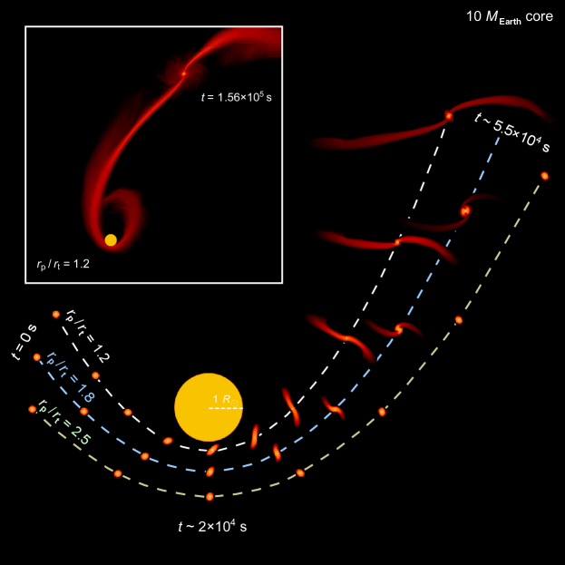
Figure 2.— Snapshots from several simulations of the tidal disruption of a Jupiter mass planet with a $10\ M_{\earth}$ core at different periastron distances. The main panel superimposes the trajectories (dashed lines) and the hydrodynamical evolution of the planet in the stellar tidal field as it flies by the star (from left to right), with the pericenter separations $r_{\rm p}$ being is $1.2\ r_{\rm t}$, $1.8\ r_{\rm t}$ and $2.5\ r_{\rm t}$, respectively. After the encounter, mass is stripped from the planet through the inner ($L_{1}$) and outer Lagrange point ($L_{2}$) and forms the two tidal streams. The material flowing through $L_{1}$ then falls back to the host star and is eventually accreted (inset panel). The yellow filled circles represent the position and size of the star, taken here to be equal to that of the Sun.

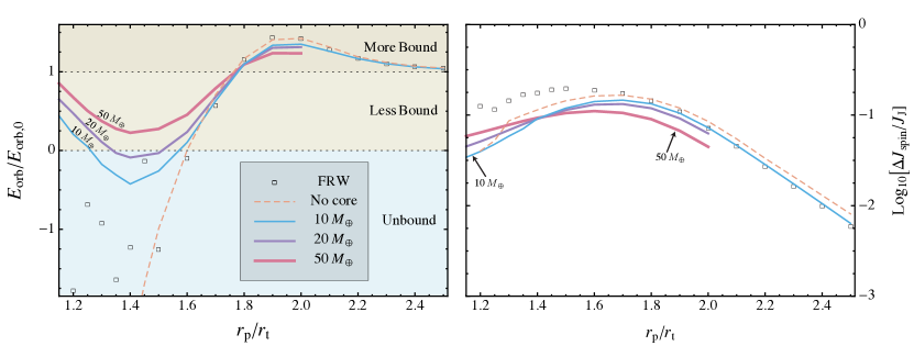
Figure 3.— Final specific orbital energy $E_{\rm orb}$ scaled to the initial specific orbital energy $E_{\rm orb,0}$ (left panel) and spin angular momentum $J_{\rm spin}$ scaled by the characteristic angular momentum of Jupiter $J_{\rm J}^{2}=GM_{\rm J}^{3}R_{\rm J}$ (right panel) as functions of periastron distance $r_{\rm p}$ in units of tidal radius $r_{\rm t}$ after a single near-parabolic encounter between a $M_{\rm P}=M_{\rm J}$ planet and a $M_{*}=10^{3}\ M_{\rm J}$ star. Open squares show the data for coreless planets as presented in FRW, whereas the dashed line shows the results of GRL. The three colored solid lines show the results from disruption simulations of Jupiter-like planets with core masses of 10, 20, and 50 $M_{\oplus}$, respectively. The filled regions in the left-hand panel show the three possible outcomes: The planet either becomes more bound, less bound, or completely unbound from its parent star after the encounter.

We carry out numerical simulations to follow the hydrodynamic response of gas giant planets during their close encounters with their host stars. Our simulations are constructed based on the framework of FLASH (Fryxell et al., 2000), an adaptive-mesh, grid-based hydrodynamics code (a good introduction to grid-based numerical methods is given in Bodenheimer et al., 2007). The simulation of tidal disruptions within the FLASH framework was initially outlined in Guillochon et al. (2009). In that work, the disruption of stars by supermassive black holes (SMBHs) were simulated for the purpose of characterizing the shock breakout signature resulting from the extreme compression associated with particularly strong encounters. In GRL the code was adapted to simulate the effects of strong tides on giant, coreless planets after both single and multiple close-in passages. Recently, (Guillochon & Ramirez-Ruiz, 2012; MacLeod et al., 2012) used this same code formalism to determine the feeding rate of supermassive black holes from the disruptions of both main-sequence and evolved stars at various pericenter distances.

In this work, we further extend the numerical framework presented in the above references to include the ability to simulate multi-layered objects, with each layer obeying a separate equation of state (EOS). As before, we treat the star as a point-mass (Matsumura et al., 2008), and the simulations are performed in the rest-frame of the planet to avoid issues relating to the non-Galilean invariance (GI) of the Riemann problem (Springel, 2010). Our planets are modeled using composite polytropes (as described in Section 2), and we further assume that the adiabiatic indices are equal to the polytropic indices. This provides a reasonable approximation to the structures of Jupiter-like planets (Hubbard, 1984).

The total volume of the simulation box is $10^{13}\times 10^{13}\times 10^{13}\;\textrm{cm}^{3}$. The initial conditions are identical to that of FRW and GRL to facilitate comparisons. The planet is assumed to have a mass $M_{\rm P}=M_{\rm J}$ and a radius $R_{\rm P}=R_{\rm J}$, where $M_{\rm J}$ and $R_{\rm J}$ are Jovian mass and radius, respectively. The planets are disrupted by a star with $M_{*}=10^{3}\ M_{\rm J}\simeq 0.95\ M_{\sun}$. Thus, the tidal radius of the planet is $r_{\rm t}=10\ R_{\rm J}\simeq 0.995\ R_{\sun}=0.00463$ AU.

We set the initial orbit of the incoming planet to have an apastron separation $r_{\rm a}=10^{4}\ R_{\rm J}$. At the onset of the simulation, we set the distance of the planet from the star to be 5 $r_{\rm t}$ such that tides are initially unimportant, and also assume that the planet has no initial spin in the inertial frame.

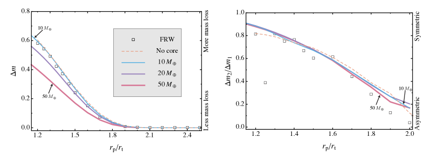
Figure 4.— Total mass fraction lost from Jupiter-like planets of varying core masses as a function of $r_{\rm p}/r_{\rm t}$. The left panel shows $\Delta m$ the total mass fraction unbound from the planet, whereas the right panel compares the ratio between $\Delta m_{2}$, the fraction of mass lost from $L_{2}$, to $\Delta m_{1}$, the fraction of mass lost from $L_{1}$. The color scheme and line style are the same as in Figure 3.

3.2. Results

In total, we simulated 41 models with the three different core masses listed in Table 1 and the initial periastron distance $r_{\rm p}$ ranging from 1.15 to 2.5 $r_{\rm t}$. A selection of simulations for $M_{\rm core}=10\ M_{\oplus}$ is illustrated in Figure 2. To explore the effect of the polytropic index of the core on the dynamics of the encounter, we simulate one additional 10 $M_{\oplus}$ model using $n_{1}=0.01$, with $r_{\rm p}=1.2\ r_{\rm t}$. Despite the radically different adiabatic index, we found less than a 1% difference between the small $n_{1}$ and our fiducial larger $n_{1}$ in terms of changes in orbital energy and mass loss. Thus, our results are not sensitive to relatively large value of $n_{1}$ used in our simulations, which was chosen for numerical convenience. This approximation is not expected to affect any of the results presented here, and should remain appropriate as long as the core is much denser than the envelope and can retain a significant amount of mass, which is always true in our single passage simulations. However, this may not be valid if the mass loss is large, as may be the case for multiple passages. The reader is refer to Section 4.2 for a detailed explanation of the adiabatic response of composite polytropes to mass-loss and its relevance in describing the outcome of multiple passage encounters.

3.2.1 Final Orbits of Disrupted Giant Planets

In all our simulations, the planet is placed on a bound orbit with a negative orbital energy per unit mass $E_{\rm orb,0}$. We plot in the left panel of Figure 3 the ratio of $E_{\rm orb}/E_{\rm orb,0}$, where $E_{\rm orb}$ is the energy per unit mass at the end of the simulation, approximately 50 dynamical timescales after pericenter. A planet’s orbit is more (less) gravitationally bound to its host star if this ratio attains a positive value greater (lesser) than unity. A planet becomes unbound if this ratio attains a negative value. For comparison with previous simulations, we show the results obtained by FRW with open squares and those of single-layered polytropes obtained by GRL with orange dashed lines in Figure 3. The results of the new simulations with $10M_{\oplus}$, $20M_{\oplus}$ and $50M_{\earth}$ cores are shown as colored solid lines.

We find that while the addition of a core produces qualitatively different results than coreless models, there are no qualitative differences when the core mass is varied for the values investigated here. The results in the left panel of Figure 3 show that for planets with a 10 $M_{\oplus}$ core, the magnitude of $E_{\rm orb}/E_{\rm orb,0}$ is greater than unity, i.e. the planet becomes more bound, for all encounters with $r_{\rm p}/r_{\rm t}\gtrsim 1.75$, approaching unity for distant encounters where $r_{\rm p}\gg r_{\rm t}$. For encounters with $1.57\lesssim r_{\rm p}/r_{\rm t}\lesssim 1.75$, this ratio remains positive but below unity, and thus these planets become less bound to their host star. For $1.27\lesssim r_{\rm p}/r_{\rm t}\lesssim 1.57$, planets become unbound, whereas those with $1.15\lesssim r_{\rm p}/r_{\rm t}\lesssim 1.27$ lose approximately half of their initial mass, yet remain bound to their host stars.

The non-monotonic relationship between $r_{\rm p}$ and the change in orbital energy is considerably more complex than the results presented in FRW or GRL, where a coreless giant planet was assumed. Although the results of encounters with $r_{\rm p}/r_{\rm t}\gtrsim 1.75$ are in general agreement with the coreless models, the discrepancy is apparent for closer encounters. These previous studies predicted that the planet becomes successively less bound when the periastron separation decreases, and all encounters with $r_{\rm p}/r_{\rm t}\lesssim 1.62$ lead to ejection. In contrast, our work suggests that for orbits with $1.4\lesssim r_{\rm p}/r_{\rm t}\lesssim 1.7$ the planet becomes successively less bound until reaching a transitional point at $r_{\rm p}/r_{\rm t}\sim 1.4$. Interior to this separation, the trend is reversed, with the orbit becoming less unbound until $r_{\rm p}/r_{\rm t}\sim 1.27$, where the planet’s orbital binding energy is comparable to its initial binding energy. A similar but more pronounced trend is found for planets with $20M_{\earth}$ and $50M_{\earth}$ cores. The more massive the core is, the more unlikely the planet will be ejected.

For planets with a $50\ M_{\earth}$ core, we find that a Jupiter-mass planet cannot be ejected in all cases we investigated with the assumed initial apastron, which we presumed to be equal to the host star’s ice line. The location of the $E_{\rm orb}=0$ crossing points as a function of $r_{\rm p}$ (Figure 3) depends on how the planet’s self-binding energy compares to its initial orbital energy. Changing the size of the planet, the ratio of the mass between the star and the planet, or the initial eccentricity can alter the normalization of $E_{\rm orb}/E_{\rm orb,0}$. For example, a smaller initial binding energy can facilitate more planetary ejections, whereas an initially more bound planet may not be capable of being ejected for any $r_{\rm p}$.

An intriguing aspect of the work presented here is that if a dense core is present, a giant planet can remain bound to the star within certain limits of periastron separation, whereas previous simulations (e.g., FRW and GRL) suggested that planets without a core are always ejected or destroyed if any mass is lost during the initial inspiral. The presence of the core permits planets to plunge deeply into their parent star’s tidal field and potentially survive as a close-in planet on a circular orbit.

It is desirable to study how does the orbit of the tidally disrupted planet evolve during subsequent encounters. But due to the extremely long orbital period of the highly eccentric giant planet ($T_{\rm orbit}/T_{\rm simulation}\sim 10^{4}$), numerical simulations that try to directly follow several orbits of the disrupted remnants are currently prohibitive. It is not clear yet whether these (marginally) bound planets will be circularized or ejected after several encounters. GRL simulated the multiple passages with a lower eccentricity ($e=0.9$), and these planets were found to be destroyed eventually after several close encounters. We do not repeat the multiple passage simulation with a lower eccentricity in this work, however, in Section 4.2 we study the adiabatic response of composite polytropes to mass-loss and use the results in Section 4.3 to explain why the presence of a dense core helps prevent planets from being destroyed in subsequent passages. This in stark contrast to the results of our previous simulations which show that core-less planets are always tidally destroyed.

The right panel of Figure 3 shows the change in spin angular momentum of the planet $J_{\rm spin}$ scaled by that of Jupiter. The planet is set to be non-rotating initially. Our hydrodynamic simulations show for Jupiter-mass planets with 10 $M_{\earth}$ and 20 $M_{\earth}$ cores $J_{\rm spin}$ peaks at around $1.7\ r_{\rm t}$, and for those with 50 $M_{\earth}$ cores $J_{\rm spin}$ peaks at around $1.6\ r_{\rm t}$. This maximum arises from the combination of the fact that smaller periaston distances result in larger tidal torques and increased mass loss. With a larger core, the planet is less distorted and at close separations the mass loss is also suppressed (Section 3.2.2), so at further separations the tidal torque is reduced and the peak shifts toward closer separations.

3.2.2 Mass Loss and Its Asymmetry

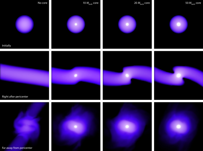
Figure 5.— Snapshots from disruption simulations of Jupiter-mass giant planets with different core masses, modeled as a dual-layered composite polytropes. Four simulations are shown above (one per column), with the only difference between the simulations being the mass of the planet’s core (as labeled). The top row shows the initial structure of the planet prior to being tidally perturbed, the middle row corresponds to the state of the planet shortly after pericenter, and the last row shows the planet many dynamical timescales after pericenter. The planet comes within 1.2 $r_{\rm t}$ of its parent star in each of the simulations, and is initialized with two separate components: A core with a stiff gamma-law EOS ($\gamma_{\rm 1}=3$, shown in white), and an envelope with a softer equation of state ($\gamma_{\rm 2}=2$, shown in purple).

Planets lose mass as a consequence of intense tidal perturbation, especially during close encounters ($r_{\rm p}<2.0\ r_{\rm t}$) as illustrated in Figure 2. This mass loss is not symmetric and, as suggested by FRW and GRL, is responsible for the observed change in $E_{\rm orb}$. The resultant kick from asymmetric mass loss will be discussed in detail in Section 4.1. The fraction of mass unbound from the planet $\Delta m$ in each run is plotted in the left panel of Figure 4. The results show that for encounters with $r_{\rm p}\geq 2.0\ r_{\rm t}$, tides raised by the star are too weak to shed any noticeable amount of mass from the planet, irrespective on its internal structure. However, in the mass-shedding regime ($r_{\rm p}<2.0\ r_{\rm t}$), the discrepancies between different models are rather prominent. Although the presence of a core does not alter the total mass and radius of the planet, planets with cores heavier than 20 $M_{\earth}$ lose significantly less mass than those without cores. In the case of a $50\ M_{\earth}$ core (corresponding to 15% of the total mass), the planet can retain more than half of its mass even for the deepest encounter we calculated in this work, with a periastron separation of only $1.15\ r_{\rm t}$. Note that the stellar radius imposes a lower limit on the planet’s minimum periastron approach distance; i.e., the sum of star’s and planet’s radii $R_{*}+R_{\rm P}\simeq 1.0995\ R_{\sun}\simeq 1.105\ r_{\rm t}$, assuming the host star is Sun-like and has a radius of $1\ R_{\sun}$.

As a result of the local strength of the tidal field being proportional to $r^{-3}$, $\Delta m_{1}$, the fraction of mass lost through $L_{1}$, is always greater than $\Delta m_{2}$, the fraction of mass lost through $L_{2}$ ($\Delta m=\Delta m_{1}+\Delta m_{2}$). We plot the ratio of the mass lost in the two tidal streams $\Delta m_{2}/\Delta m_{1}$ as a function of the periastron separation in the right panel of Figure 4. We confirm the change of asymmetry of mass loss as first noted by FRW, in which the inner stream dominates mass loss at large separations where the total mass loss is small, while $\Delta m_{2}/\Delta m_{1}$ approaches unity (but is still less than one) at smaller separations where the total mass loss is significant. This is also reflected in the morphological difference between disrupted planets illustrated in Figure 2 by the two trajectories $r_{\rm p}/r_{\rm t}=1.2$ and $r_{\rm p}/r_{\rm t}=1.8$. All the models with different core masses generally conform to this trend, albeit models without cores seem to deviate from models with cores for both small and large values of $r_{\rm p}/r_{\rm t}$, with the change in energy increasing dramatically for the former and saturating at a fixed value for the latter. Note that the mass loss difference may be modified by the magnitude and orientation of incoming planets’ spin if the spin frequency is a significant fraction of that for break up, with the spin potentially being accumulated over prior encounters with the star (Figure 3).

3.2.3 Core Mass and Survivability

Planets with cores not only lose less mass, but also maintain their internal structures more effectively than their coreless counterparts after the disruption has occurred. Figure 5 shows density profiles of various planet models as they are torn apart near their pericenters (middle row), and when the remnants are relaxed after many dynamical timescales (bottom row). Without a core (first column), the planet is easily shredded, resulting in a long tidal stream that eventually coalesces into a weakly self-bound remnant. The envelope of a planet with a core is still significantly disturbed at pericenter, but the core itself is only weakly affected (second through fourth columns). This results in a core-envelope interface that is well-preserved after the encounter, with planets maintaining a larger fraction of their original structure for progressively larger core masses.

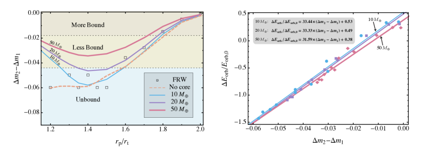
Figure 6.— The left panel shows the difference between the two normalized mass loss $\Delta m_{2}-\Delta m_{1}$ as a function of periastron distance scaled by the tidal radius $r_{\rm p}/r_{\rm t}$. The color bands have the same meaning as in the left panel of Figure 3. The correlation between the mass loss difference $\Delta m_{2}-\Delta m_{1}$ and changes in orbital energy scaled to the initial specific orbital energy $\Delta E_{\rm orb}/E_{\rm orb,0}$ is shown in the right panel, where the orange triangles, blue points, purple squares and red diamonds are the simulation data of planets with no core, $10\ M_{\earth}$, $20\ M_{\earth}$ and $50\ M_{\earth}$ cores respectively. The blue thin, purple medium, and red thick lines show the linear least squares fits to the simulations with cores.

Cores have long been ignored in hydrodynamic simulations because they only contribute to a tiny fraction of a planet’s total mass, and have thus been thought to be dynamically insignificant. However, we show that the core mass is of prime importance in determining the fate of disrupted planets in the sense that both the changes in orbit energy and morphology of the planets are strongly related to their cores. The addition of cores to models of giant planets may be the key to solving the overestimated destructiveness of tidal field found in GRL. We shall discuss the effects of cores in the context of a planet’s adiabatic response to mass loss in Section 4.3.

4. Discussion

4.1. The correlation between mass loss and changes in orbital energy

The left panel of Figure 6 shows the normalized mass difference between the two streams $\Delta m_{2}-\Delta m_{1}$ as a function of the periastron separation for various planet models. The mass difference $\Delta m_{2}-\Delta m_{1}$ can be related to the total mass loss $\Delta m$ and the mass loss ratio $\Delta m_{2}/\Delta m_{1}$ through a simple relation

$$\Delta m_{2}-\Delta m_{1}=-\Delta m\left(\frac{2}{\Delta m_{2}/\Delta m_{1}+1}-1\right).$$ (17)

Because $\Delta m$ is a monotonically decreasing function of $r_{\rm p}/r_{\rm t}$, while the term in the parentheses on the right hand side of equation (17) is a monotonically increasing function of $r_{\rm p}/r_{\rm t}$, the mass difference maximizes (i.e. $\Delta m_{2}-\Delta m_{1}$ becomes most negative) for planets with cores when $r_{\rm p}/r_{\rm t}\simeq 1.4$. One may notice that the dependence of $\Delta m_{2}-\Delta m_{1}$ on periastron separation is very similar to that of $E_{\rm orb}/E_{\rm orb,0}$. Indeed, we find the change in specific orbital energy scaled to the initial specific orbital energy $\Delta E_{\rm orb}/E_{\rm orb,0}$ linearly correlates with the normalized mass difference $\Delta m_{2}-\Delta m_{1}$, where $\Delta E_{\rm orb}=E_{\rm orb}-E_{\rm orb,0}$ is the change in specific orbital energy after the tidal disruption (Fitting formulas are provided in Figure 6 for reference). Thus, one may use the mass difference to determine whether a planet’s final orbit is more bound or less bound, as illustrated in color-shaded regions in the left panel of Figure 6.

What underlies this linear relation is energy conservation. Material stripped from the planet with negative binding energy becomes bound to the host star and forms the inner tidal stream, while that with positive binding energy becomes unbound to the system and forms the outer tidal stream. Not surprisingly, the energy deposited into the inner tidal stream is always greater than that deposited into the outer stream due to the asymmetric tidal forces, with the degree of asymmetry depending on the ratio between the star and the planet’s masses. As a result, the change in planet orbital energy reflects the binding energy difference between the two streams as the total system’s energy must be conserved. For all cases with mass loss, the net energy exchange between the two tidal streams is negative, resulting in a positive change in the planet’s orbital energy. Thus, the planet becomes less bound (or unbound) to the star assuming any other form of energy exchange can be neglected. This assumption holds for all deep encounters with large mass loss.

However, two additional sinks of energy exist: The energy stored within the planet’s normal modes of oscillation $E_{\rm osc}$, and the energy associated with the planet’s final spin $E_{\rm spin}$. The sum of these two terms cannot exceed the planet’s own self-binding energy, $E_{\rm bind}\simeq GM_{\rm P}^{2}/R_{\rm P}$, and this reflects the maximum negative change in orbital energy that can be achieved in a single passage. As we show in the right panel of Figure 3, planets gain most spin angular momentum at separations where the mass loss is relative small. In other words, the rotational and oscillatory kinetic energies saturate for encounters in which little mass is lost, and thus cannot aid in retaining the planet for deeper encounters.

Because the asymmetric mass loss could kick the planet into a less bound orbit, one may conclude that the continuous positive change in the planet’s orbital energy could lead to a planetary ejection after several close-in passages. However, this statement overlooks several crucial facts. First, the planet loses a significant fraction of its mass during the first passage, leading to an increase in the mass ratio of subsequent encounters. Second, while the planet’s envelope becomes progressively less dense after each encounter, the core remains intact. As a result, the thrust provided by the loss of the envelope becomes less effective as its mass decreases (the effects of the core on the survivability of the planet will be discussed in Section 4.2). As the envelope is depleted, the effective tidal radius $r_{\rm t}$ increases. Consequently, in the following passages the planet may have $r_{\rm p}/r_{\rm t}$ values close to or even less than unity, and the two tidal streams produced by subsequent encounters will be more equal in mass, as suggested by our simulations (see Figure 6). As the ratio of core mass to total mass is enhanced, this results in a larger specific self-binding energy for material close to the core-envelope interface, and if this material is perturbed, it can absorb a larger fraction of the planet’s orbital energy. As a result, the specific orbital energy may become more negative than in the case where no core is present. We also did not consider the possibility that planets are scattered from distances inside their parent stars’ respective snow lines. In those cases, the energies required to unbind the planets are much larger than the energy exchanged in the encounter, and planets are more likely to be bound to the star, even after multiple passages.

4.2. Adiabatic Responses of Mass-losing Composite Polytropes

When a planet loses mass on a timescale faster than the Kelvin-Helmholtz time but slower than the dynamical time, the structure of the planet will evolve adiabatically so that the entropy as a function of interior mass is approximately conserved (Dai et al., 2011). Hjellming & Webbink (1987) used composite polytropic stellar models ($P\propto\rho^{\gamma}\propto\rho^{1+{1\over n}}$) to explore the stability of this adiabatic process. We have modified their formalism slightly by taking into account a distinct chemical composition between the core and envelope, $\mu_{1}=4\ \mu_{2}$. We also consider a different combination of polytropic indices, $n_{1}=0.01$ and $n_{2}=1$. Note here we choose the more realistic value of $n_{\rm 1}=0.01$ instead of $n_{\rm 1}=0.5$ used in our hydrodynamic simulations, because we want to investigate the extreme case in which the entire envelope is shed. A stiff EOS is required in order to capture the core’s incompressible response to pressure deformations. The reader is refer to Appendix A for a detailed description of our adiabatic response to mass loss model for composite polytropes.

In contrast to the single-layered $n=1$ polytrope, which has a constant radius, composite polytropes with a small $n_{\rm 1}$ always contract as they lose mass. As illustrated in Figure 7, the planet’s contraction rate is observed to increase as the core mass fraction increases. The way that a planet evolves and ends up in such a tidally mass-losing environment depends upon how its mean density (or size) changes as it losses mass. The dotted line in Figure 7 denotes the boundary below which the adiabatic response will lead to an increase in the mean density of the stripped planet and, as a result, the stripped object will be less vulnerable to tidal disruption. However, during the tidal circularization process the planet’s periastron distance $r_{\rm p}$ will increase due to conservation of orbital angular momentum. Once $r_{\rm p}$ becomes sufficiently large (say about $2.5\ r_{\rm t}$) such that stellar tides can no longer strip significant mass from the planet, a lower mean density could still arise as a result of tidal heating.

Figure 7 can help explain the dependence of our results on the assumed polytropic index of the core. The computed coreless model is equivalent to the composite polytrope with an $n_{1}=1$ core (ignoring of course that there is no density jump at the core-envelope interface in this model). Thus, one can qualitatively infer that the adiabatic response of a core’s model with $0.01<n_{1}<1$ would lie between the two model extremes represented in Figure 7. By doing so we see that only a very small discrepancy in the adiabatic responses of the extreme models depicted in Figure 7 can be observed until as much as half of the mass of the planet is lost ($M/M_{\rm P}\sim 0.5$). This gives credence to the idea that our results are rather insensitive to $n_{1}$, because the overall adiabatic response is mainly determined by the remaining envelope, which is at least an order of magnitude more massive than a 10 $M_{\earth}$ core. This is consistent with our additional hydrodynamic simulation, where no dramatic difference between models with $n_{1}=0.5$ and $n_{1}=0.01$ was found after a single close encounter.

As the mass loss increases, the mass of the core becomes progressively more important in determining the adiabatic response of the planet. When the mass of the remaining envelope becomes comparable to the mass of the core, the overall response of the composite polytrope to mass loss is primarily dictated by the core. At this stage, models with different $n_{1}$ behave very differently. For these extremes cases, a small $n_{1}=0.01$ is more suitable to model the incompressible behavior of a rocky core.

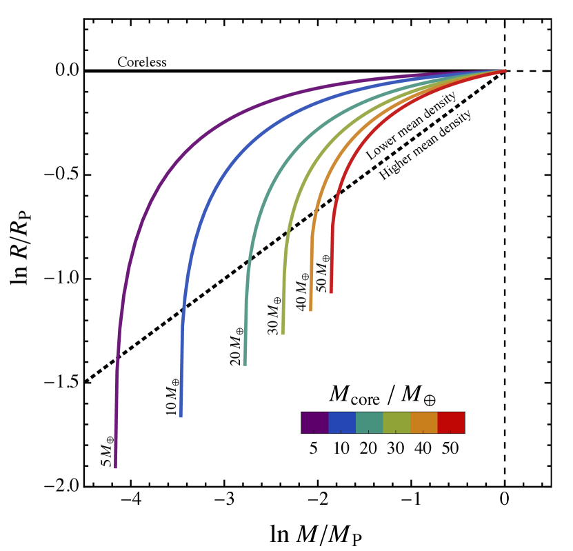
Figure 7.— Adiabatic response curves for composite polytropes for varying degrees of mass loss. All curves start from the origin (zero mass loss). A negative value indicates either a decrease in mass (x-axis) or a shrinkage of the planet’s radius (y-axis). The top horizontal thick black line shows the evolution for a single-layered $n=1$ polytrope model. From left to right the solid lines in colors are the response curves of composite polytropes with 5, 10, 20, 30, 40, and $50\ M_{\earth}$ cores, respectively. For all the composite polytrope models, we assume $n_{\rm 1}=0.01$ and $n_{\rm 2}=1$, and set the two layers to have different molecular weights, with $\mu_{\rm 1}=4\ \mu_{\rm 2}$. The dotted line (whose slope is 1/3) illustrates the response required to have no noticeable change in the planet’s mean density. Below this line, composite polytropes become more dense in response to further mass loss.

4.3. The Role of Dense Cores

Our hydrodynamical simulations have demonstrated that with larger cores, planets retain a greater fraction of their original envelope (see Figure 5 for comparison), which also means that the difference between the mass lost from the near- and far-sides of the planet is reduced, and therefore the planet has a greater chance to be bound to the host star. This result is somewhat surprising as the cores contain only a small fraction of the planet’s total mass, and have been regarded as being dynamically unimportant (e.g. FRW and GRL). Previous studies which have attempted to determine the final fate of disrupted hot Jupiters usually ignore the complexity of the planet’s interior structure.

Recently, Remus et al. (2012) investigated the dissipative equilibrium tide in gas giant planets by taking into account the existence of viscoelastic cores. While approaches similar to theirs can predict the amount of energy deposited into a planet’s interior by an external tidal perturber, such formalisms fail for disruptive encounters in which non-linear dynamical effects dominate and a significant fraction of mass is removed from the planet. To approximate dynamical mass loss, we calculate the adiabatic response of composite polytropes. Cooling is ignored in our analysis as its time scale is significantly longer than the dynamical time scale (Bodenheimer et al., 2001), but we note that it can be important in determining the planet’s final structure once mass loss ceases (Fortney et al., 2007).

The $n=1$ single-layered polytrope, which corresponds to the coreless gas giant planets, does not change its radius when losing mass adiabatically, resulting in a decrease of the average density. By contrast, the extremely incompressible cores of composite polytropes are weakly affected by the perturbation, imposing an almost constant inner boundary condition for the envelope, and resulting in an increase in density when the core’s gravity dominates (see Figure 7). This phenomenon helps to explain the different amounts of mass lost in the two cases. Each time the single-layered polytrope loses some mass, the specific gravitational self-binding energy decreases, leading to a more tidally-vulnerable structure. As a result, GRL found that coreless planets are always destroyed after several passages even if the initial periastron is fairly distant (the lower limit is $2.7\ r_{\rm t}$). The composite polytropes, on the other hand, maintain a constant gravitational potential well in their centers, which continuously resists the stellar tidal force. Being invulnerable to tidal disruption themselves, the cores survive, retaining some fraction of the original envelope (MacLeod et al., 2012). This results in a core mass fraction that is significantly larger than that of the original planet.

We should emphasize that although we focus on Jupiter-mass planets in this work, the scenario presented here can apply to giant planets of different masses, as long as they are characterized by a similar dual-layered structure. There are several known gas giant planets with very large average densities and enhanced metallicities (Bakos et al., 2011). CoRoT-20 b, for instance, with a core mass fraction between 50% and 77% of its total mass, orbits a G-type star on an eccentric orbit ($e=0.562$) (Deleuil et al., 2012). It is not clear yet how these metal-rich giant planets are formed. Tidal disruption might be an explanation. In this scenario, these planets were more massive prior to disruption, with a more typical fraction of heavy elements concentrated in their cores. After the loss of the envelope, the planet’s average properties, including metallicity, become more representative of the core’s initial properties. Measurements of the metallicity enhancement, combined with measurements of the planet’s orbital properties, may enable one to infer the planet’s original mass.

4.4. Demographics of the Surviving Tidally Disrupted Giant Planet Population

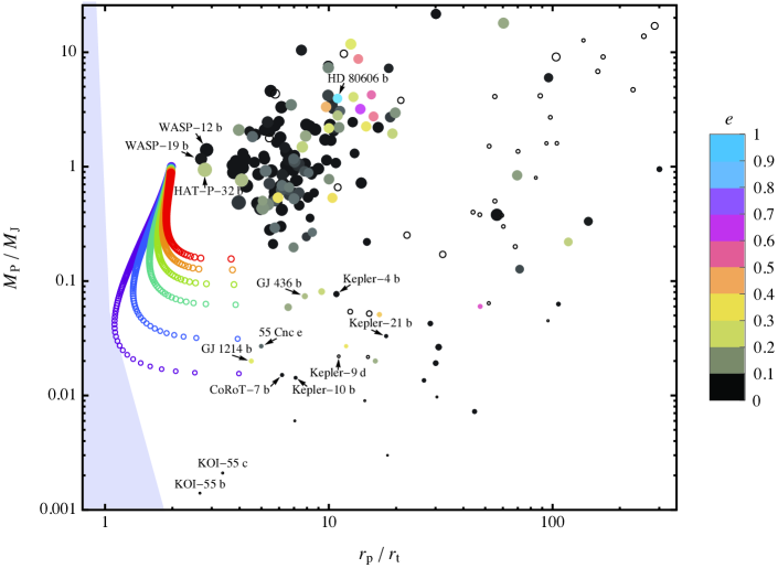
Figure 8.— Planet mass $M_{\rm P}$ versus pericenter distance $r_{\rm p}$ scaled by the tidal radius $r_{\rm t}$. The sample is composed of planets with known mass and radius and a known stellar mass, from which the tidal radius $r_{\rm t}$ for each planet is then computed. The filled points are color-coded by the planet’s eccentricity. For the planets with unknown eccentricity, $e=0$ is assumed. The open points illustrate the adiabatic evolution of a Jupiter-mass planet experiencing mass loss with different core masses, with the color coding being the same as in Figure 7. The blue shaded region in Figure 8 is plotted to illustrate how $R_{\odot}$ compares with $r_{\rm t}$ as the planet’s mass is varied, with the relationship being linearly interpolated between the Sun-Earth, Sun-Neptune and Sun-Jupiter cases. All exoplanet data was taken from the Extrasolar Planets Encyclopaedia (http://exoplanet.eu/) on June 14, 2012, the sample contains 217 planets.

Table 2A sample of extremely close-in super-Earths and Neptune-size planets

Name	$M_{\rm P}$	$R_{\rm P}$	$a$	Period	$e$	$M_{*}$	$\rho_{\small\rm P}$	$r_{\rm p}/r_{\rm t}$	$r_{\rm p,0}/r_{\rm t,0}$
	($M_{\earth}$)	($R_{\earth}$)	(AU)	(days)		($M_{\odot}$)	($\rho_{\small\rm J}$)
55 Cnc e	8.58	2.11	0.0156	0.74	0.06	0.91	3.70	4.99	1.71
Kepler-10 b	4.55	1.38	0.0168	0.84	0	0.90	6.98	7.11	1.86
CoRoT-7 b	4.80	1.63	0.0172	0.85	0	0.93	4.47	6.18	1.88
GJ 1214 b	6.36	2.66	0.014	1.58	0.27	0.15	1.36	4.51	2.58
Kepler-9 d	7.00	1.60	0.0273	1.59	0	1	6.93	11.08	2.91
GJ 436 b	23.42	3.96	0.029	2.64	0.15	0.45	1.52	7.82	3.92
Kepler-21 b	10.49	1.58	0.0425	2.79	0	1.34	10.49	18.05	4.11
Kepler-4 b	24.47	3.88	0.0456	3.21	0	1.22	1.69	10.82	4.54

4.4.1 A Census of Exoplanets with Known Mass and Radius

Despite the rapid pace of exoplanet discovery and influx of dynamical data, information on the structure of exoplanets is still limited. Both mass and radius have been determined for several hot Jupiters and super Neptunes. Although there is essentially no direct information on their internal structure, the average density of these planets is likely to be correlated with the presence of cores (Miller & Fortney, 2011).

In order to search for some clues on the role of tidal disruption during their orbital circularization process, we show a sample of exoplanets with known planetary radii $R_{\rm P}$ and masses $M_{\rm P}$ and known stellar masses $M_{*}$ in Figure 8, where the distribution of the planet’s mass as a function of its pericenter distance scaled by its tidal radius

$$\frac{r_{\rm p}}{r_{\rm t}}=\frac{a(1-e)}{(M_{*}/M_{\rm P})^{1/3}R_{\rm P}}$$ (18)

is plotted. The color-coding of the filled dots denotes eccentricity $e$, and the open black circles represent planets with unknown eccentricity, where we have assumed $e=0$ for our subsequent calculations. The size of the symbols is representative of the planet’s physical size (not drawn to scale). The most eccentric planet in our sample is HD 80606b (the current record-holder HD 20782 b with $e=0.97$ is excluded because the size of this planet has not been measured). Note that there is a non-trivial fraction of planets with substantially large eccentricities. Moreover, both the radial velocity and transit surveys are biased against the detection of highly-eccentric planets (Socrates et al., 2012), as such, the fraction of these planets is likely under-represented. It is also important to notice that the most eccentric planets are found at larger separations, though this may be enhanced by detection bias. This is consistent with the scenario that dynamical processes such as planet-planet scattering (Rasio & Ford, 1996; Chatterjee et al., 2008; Ford & Rasio, 2008) or the Kozai mechanism (Kozai, 1962; Takeda & Rasio, 2005; Naoz et al., 2011; Nagasawa & Ida, 2011) lead to the excitement of a planet’s eccentricity, while tidal dissipation can damp the planet’s eccentricity in the vicinity of the star.

Zhou et al. (2007) and Jurić & Tremaine (2008) studied the eccentricity distribution of dynamically relaxed exoplanetary systems, which can be described by a Rayleigh distribution

$$dN=\frac{e}{\sigma_{e}^{2}}{\rm exp}\left(\frac{-e^{2}}{2\sigma_{e}^{2}}\right)de,$$ (19)

where $\sigma_{e}=0.3$. This distribution has a small, but non-negligible fraction of planets with eccentricities close to unity, with the number of planets having $e=0.997$ being only a factor of about 2.5 smaller than $e=0.9$. Given the observed number of eccentric planets with $0.9<e<1$, we thus expect some super-eccentric planets with $e>0.997$. For $e=0.997$, the periastron distance for a planet scattered from the snow line given a Sun-like parent star would be $r_{\rm p}=a(1-e)=0.0075\ {\rm AU}=1.5\ R_{\odot}$. For these small separations, the budgeting of the planet’s orbital energy during a tidal encounter must account for mass loss, as the final orbital energy is strongly correlated with the properties of the ejected mass (Figure 6).

To determine the evolution of giant planets in the $(M_{\rm P}$, $r_{\rm p}/r_{\rm t})$ plane, we calculate the tidal radius of composite polytropes using the structure predicted by the response to adiabatic mass loss. An initial periastron separation $r_{\rm p}=2.0\ r_{\rm t}$ is adopted. We assume that orbital angular momentum is conserved, and that the planet ends up in a circular orbit ($a\simeq 2\ r_{\rm p}$). The tracks in Figure 8 show a Jupiter-mass planet evolving into a super-Earth or a Neptune analogue (depending on the initial core mass) as its envelope is continuously removed. The tracks show that $r_{\rm p}/r_{\rm t}$ first decreases to a minimum value as the average density of the planet decreases, but this trend reverses as the importance of the gravitational influence of the core on the remaining envelope increases (Figure 7). Note that the adiabatic response model assumes that mass is slowly removed, and that no additional energy is injected into the envelope.

Based on the models of adiabatic mass loss, it seems plausible that giant planets with cores can be transformed into either super-Earths or Neptune-like planets during their orbital circularization process. As the adiabatic model only makes predictions about the structure of the planet, the model alone is incapable of determining whether the planet would be circularized or ejected, which depends on how the mass is removed from the planet.

Depending on the initial mass of the planet and its core, the final mass and radius of the planetary remnant can vary drastically (as illustrated in Figure 8). Planets that lie near the evolutionary end states for a disrupted Jupiter-like planet are tabulated in Table 2. To determine if a planet may have a tidal disruption origin we compute its initial $r_{\rm p,0}/r_{\rm t,0}$ value assuming the specific orbital angular momentum is conserved during the circularization process, so that

$$r_{\rm p,0}\simeq a_{\rm f}/2=r_{\rm p}(1+e)=a(1-e^{2}),$$ (20)

where $a_{\rm f}$ is the semimajor axis after the orbit has been circularized. If the gas giant progenitor has Jupiter’s mean density, the initial tidal radius is then given by

$$r_{\rm t,0}=r_{\rm t}\rho_{\small\rm P}^{1/3},$$ (21)

where $\rho_{\small\rm P}$ is the presently observed density of the planet. Among these planets, 55 Cnc e, Kepler-10 b and CoRoT-7 b have $r_{\rm p,0}/r_{\rm t,0}\lesssim 2$, which guarantees that if the planet was initially similar to Jupiter it would have lost mass on its first encounter with the parent star (FRW; GRL). For planets with $2\lesssim r_{\rm p,0}/r_{\rm t,0}\lesssim 2.7$ (e.g. GJ 1214 b), prolonged tidal effects over many orbits may still lead to significant mass loss (GRL). Planets with $r_{\rm p,0}/r_{\rm t,0}\gtrsim 2.7$ are unlikely to have formed as a result of the tidal disruption of a Jupiter-like planet, unless they were significantly less dense than Jupiter, which is possible at the time of scattering as may not have had sufficient time to cool (Fortney et al., 2007).

Of the transiting super-Earths with known masses, only a few presently lie within a few tidal radii of their host stars. This may indicate that the conditions necessary to generate such planets via tidal disruption are uncommonly realized in nature. However, the sample is highly biased against low-mass planets, simply because we need transit surveys to determine the planet’s size. In addition, the eccentricities for many low-mass planets are poorly constrained, and as a result, their periastron separations may have been overestimated. This highlights the importance of conducting a survey that is capable of detecting close-in, low-mass planets, such as the Kepler mission.

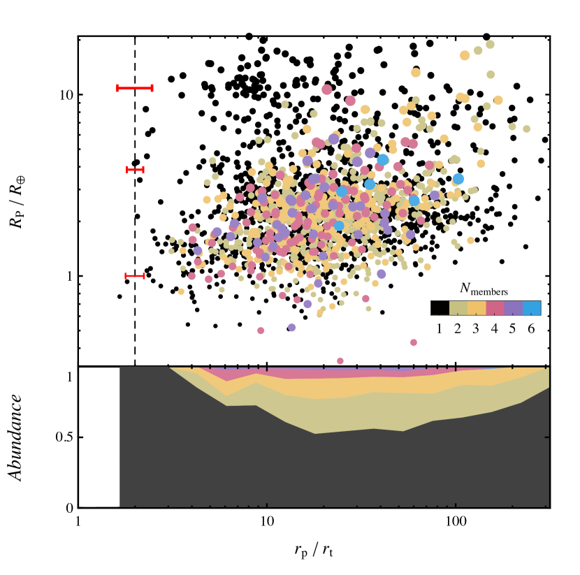
Figure 9.— The upper panel shows the radius in Earth radii of Kepler planet candidates versus pericenter distance in units of the tidal radius. The color of each point denotes the multiplicity of the system in which it resides (Batalha et al., 2012), while the dashed vertical line indicates $2r_{\rm t}$. To determine the tidal radius without explicit measurements of the mass, the density of each candidate planet is assumed to be equal to that of a similarly-sized planet in the solar system. From top to bottom, the red bars represent the range of $r_{\rm p}/r_{\rm t}$ values at typical sizes of Jupiter, Neptune and Earth, respectively (see the text for more details). In the lower panel, a stacked area plot shows the fraction of single-candidate and multi-candidate systems, with the color-coding being the same as the upper panel. All data was take from NASA Exoplanet Archive (http://exoplanetarchive.ipac.caltech.edu/).

4.4.2 A Census of Kepler Candidates

In the upper panel of Figure 9 we plot the distribution of Kepler candidate radii as a function of their periastron separations (taken to be equal to the semimajor axes) divided by their tidal radii, which we obtain making use of equation (1). Unfortunately, for most of the candidates discovered by transit we don’t known the planetary mass because usually these stars too faint to do radial velocity measurements except for those in multiple systems where transit time variation (TTV) measurement is possible (one of the successful measurement is the Kepler-11 system done by Lissauer et al. (2011)). To estimate the mass of each candidate, we use the density of planets in our solar system: For candidates whose sizes are equal or larger than Jupiter, we take the geometric mean of Jupiter’s and Saturn’s densities ($\rho_{\small\rm P}=0.96$ g cm^-3), for Neptune size candidates we use Neptune’s and Uranus’ densities ($\rho_{\small\rm P}=1.51$ g cm^-3), and for Earth and sub-Earth size candidates we use Earth’s and Mars’ densities ($\rho_{\small\rm P}=4.66$ g cm^-3). We linearly interpolate between the three cases for planets of intermediate radii. The red bars in Figure 8 show the range of $r_{\rm p}/r_{\rm t}$ values calculated with two limiting densities at each typical size. While we have assumed that the semimajor axis $r_{\rm p}=a$, Kane et al. (2012) note that some of the candidates may still have large eccentricities. However, as illustrated in Figure 8, most planets within 0.04 AU are expected to have $e\simeq 0$.

Table 3A sample of close-in Kepler candidates

KOI Name	$R_{\rm P}$	$M_{\rm P}$	$M_{*}$	$r_{\rm p}/r_{\rm t}$
	($R_{\earth}$)	($M_{\oplus}$)	($M_{\sun}$)
799.01	6.07	52.10	0.83	2.35
861.01	1.77	3.01	0.79	2.49
928.01	2.56	6.64	0.91	2.74
1150.01	1.10	1.05	1.02	2.42
1164.01	0.77	0.39	0.55	1.66
1187.01	3.38	11.95	0.80	2.12
1285.01	6.36	58.76	0.85	2.48
1419.01	8.31	115.89	0.95	2.28
1442.01	1.36	1.69	1.07	2.78
1459.01	4.17	19.42	0.58	1.99
1502.01	2.13	4.48	0.80	2.06
1510.01	1.50	2.09	0.77	2.64
1688.01	0.93	0.68	0.73	1.82
1812.01	4.57	24.78	0.93	2.31
2233.01	1.61	2.44	0.88	2.55
2266.01	1.63	2.51	0.71	2.99
2306.01	0.94	0.70	0.54	2.50
2347.01	1.01	0.86	0.55	2.37
2404.01	1.50	2.09	0.91	2.91
2492.01	0.88	0.58	1.00	2.74
2542.01	1.07	0.99	0.51	2.31
2573.01	4.24	20.31	0.64	2.05

Some candidates with sizes smaller than Jupiter have present-day orbits with $a\sim 2\ r_{\rm t}$ (indicated by the vertical dashed line in the upper panel of Figure 9), and thus are potentially the surviving remnants of tidally circularized giant planets with cores. Table 3 lists all the Kepler candidates with sub-Jupiter sizes and $r_{\rm p}/r_{\rm t}<3$ for reference.

Among Kepler cataloged stars, 20% of them have multiple planet candidates (Batalha et al., 2012). The points in the upper panel of Figure 9 are colored to display the multiplicity of the system. We do not attempt to statistically study the differences between singles and multiple systems in detail, here we simply count numbers of planet candidates for single and multiple systems and compare their relative abundances. The result is shown in the lower panel of Figure 9, where again the color denotes multiplicity. Intriguingly, the candidates found in multiple systems tend to lie further from their parent stars, and none of the candidates listed in Table 3 are observed to belong to a multiple candidate system (although they might have distant, unobserved siblings). Planets in compact multiple systems are thought to be formed through orbital migration, such as the Kepler 11 system, which hosts six planets. The fact that the distribution of the semi-major axis within a few tidal radii differs for single-candidate versus multiple-candidate systems suggests that close-in candidates may have instead formed via dynamical interaction. However, many of the single-candidate systems may be false-positives, whereas the false-positive fraction is much reduced for the multiple-candidate systems (Lissauer et al., 2012). But even under the pessimistic assumption that half of the observed close-in candidates are false-positives in Table 3, there are still around a dozen candidates in the currently available sample that are close enough to their parent stars to have had a strong tidal encounter in which much of their original mass was lost. The conformation of these candidates as true planets opens the possibility that they have undergone a radical transformation.

In principle, difference in formation histories may be used to distinguish between the residual cores of gas giant planets and the failed cores which failed to accrete significant amounts of gas. For example, under high pressure, metals may react with hydrogen to produce metallic hydrides such as iron hydride (Badding et al., 1991, Q. Williams 2012, private communication), which would reduce the core’s mean density from that of a pure metal composition. These reactions are not expected to happen in failed cores and might be the only discernible signature as the difference in planetary densities between these two scenarios may be too small to be observable.

5. Summary

Nayakshin (2011) studied the scenario that the tidal disruption of giant planets occurs during the migration phase of planetary formation. Under this scenario, the planets migrate inwards faster than their cooling timescales, and are disrupted before they can contract and become more resistant to tides. However, if these planets underwent disk migration, all close-in planets should have eccentricities near zero. But as there seems to be an eccentricity gradient, with non-zero eccentricities being sustained for planets just exterior to their present-day tidal radii, dynamical interactions followed by dissipative processes that depend on the distance to the host star offer an attractive explanation for producing the observed hot Super-Earths, Neptunes, and Jupiters. While it is unknown if other effects can produce the observed eccentricity distribution, scattering events that place planets onto disruptive orbits are likely to occur in some fraction of planetary systems.

In this paper, we presented three-dimensional hydrodynamical simulations of the disruption of giant planets. In contrast to previous work, we model the planets by including the dense cores that may exist in the interiors of many (if not most) giant planets. We show that cores as small as $10M_{\earth}$ can increase both the fraction of planets that survive, and the fraction that remain bound to the host star after a tidal disruption, and that larger cores make such outcomes more probable. This is contrary to what has been predicted by previous simulations in which the giant planets were assumed to be without cores, where the planets were found to receive large kicks that would eject them from their host stars, and/or be destroyed in the process (FRW and GRL). We show that the change in orbital energy is linearly related to the difference in mass between the two tidal streams, suggesting that simple energy conservation arguments are sufficient to explain the observed post-disruption kicks. We compared our results to the adiabatic response of composite polytropes to mass loss, and find that while coreless planets always expand in response to mass loss, planets with cores contract, allowing them to retain a fraction of their initial envelopes.

Based on these results, we propose that some gas giant planets with dense cores could be effectively transformed to a super-Earth or Neptune-size object after multiple close encounters. Some of these transformed planets may already exist within the currently known sample of exoplanets, and are expected to be small, dense objects that lie close to their parent stars. The paucity of very close-in exoplanet candidates in multiple systems found by Kepler might suggest that the ordered, gentle migration that typifies most of these systems may not be universal, and that some systems may evolve via intense periods of dynamical evolution. One possible signature of such a dynamical intense event may be an enhancement of the stellar metallicity as a result of chemical pollution (Li et al., 2008), or a misalignment between the planet’s orbit and the parent star, as is measured via the Rossiter-MacLaughlin effect. If it can be determined that some of the observed sample of close-in Neptunes and super-Earths are relics of this dynamical history, we may be better equipped to understand the nature of late-phases of planetary formation.

Appendix A Adiabatic Response of Composite Polytropes with Distinct Chemical Compositions

Adiabatic responses of composite polytropes to mass loss in the context of binary systems have been investigated by Hjellming & Webbink (1987). They introduced a parameter $w$ to represent variations in the central pressure, and solved the Lane-Emden equation in a set of Lagrangian coordinates. We incorporate their formalism and use separate molecular weights ($\mu_{1}$ and $\mu_{2}$) for the core and envelope to represent their distinct chemical compositions. Following their notations, the continuity equations (equation (22) and (23) in their work) become

$$\frac{x_{1}}{\theta_{1}}\frac{d\theta_{1}}{dx_{1}}=\frac{x_{2}}{\theta_{2}}\frac{d\theta_{2}}{dx_{2}},$$ (A1)

$$x_{1}\theta_{1}^{\frac{n_{1}-3}{6(n_{1}+1)}}\mu_{1}^{-2/3}=x_{2}\theta_{2}^{\frac{n_{2}-3}{6(n_{2}+1)}}\mu_{2}^{-2/3}.$$ (A2)

We have following conditions at the core-envelope interface:

$$x_{2}=x_{1},$$ (A3)

$$\theta_{2}=\theta_{1}^{\lambda}\left(\frac{\mu_{1}}{\mu_{2}}\right)^{-\frac{2}{3}},$$ (A4)

$$\frac{d\theta_{2}}{dx_{2}}=\frac{d\theta_{1}}{dx_{1}}\theta_{1}^{\lambda-1}\left(\frac{\mu_{1}}{\mu_{2}}\right)^{-\frac{2}{3}},$$ (A5)

where

$$\lambda\equiv\left(\frac{n_{1}-3}{n_{2}-3}\right)\left(\frac{n_{2}+1}{n_{1}+1}\right).$$ (A6)

For comparison with the hydrodynamical simulations we choose the ratio of mean molecular weight between core and envelope $\mu_{1}/\mu_{2}=4$.

The combination of polytropic indices in their work is not suitable for modeling a planet. Here, we have chosen $n_{1}=0.01$, $n_{2}=1$, and $\gamma_{1}=1+1/n_{1}=101$, $\gamma_{2}=1+1/n_{2}=2$. The reason we did not use the same polytropic index for the core as in the simulations is that we want to study the extreme case in which the entire envelope would be shed, to model the incompressible core we need a extremely large $\gamma$.

The perturbed polytrope is described by

$$\omega(x)\equiv P(x)/P_{0}(x)=(\rho/\rho_{0})^{\gamma},$$ (A7)

where subscript 0 denotes the unperturbed polytrope. The continuity requirements are:

$$\omega_{2}=\omega_{1},$$ (A8)

$$\frac{d\omega_{2}}{dx_{2}}=\frac{d\omega_{1}}{dx_{1}}.$$ (A9)

The overall tendency of the composite polytrope to shrink or expand is determined by the competition between each component (Hjellming & Webbink, 1987).

References

- Badding et al. (1991) Badding, J. V., Hemley, R. J., & Mao, H. K. 1991, Science, 253, 421
- Bakos et al. (2011) Bakos, G. Á., et al. 2011, ApJ, 742, 116
- Batalha et al. (2012) Batalha, N. M., et al. 2012, ArXiv e-prints
- Bodenheimer et al. (2007) Bodenheimer, P., Laughlin, G. P., Rózyczka, M., & Yorke, H. W. 2007, Numerical Methods in Astrophysics: An Introduction
- Bodenheimer et al. (2001) Bodenheimer, P., Lin, D. N. C., & Mardling, R. A. 2001, ApJ, 548, 466
- Chatterjee et al. (2008) Chatterjee, S., Ford, E. B., Matsumura, S., & Rasio, F. A. 2008, ApJ, 686, 580
- Dai et al. (2011) Dai, L., Blandford, R. D., & Eggleton, P. P. 2011, ArXiv e-prints
- Deleuil et al. (2012) Deleuil, M., et al. 2012, A&A, 538, A145
- Faber et al. (2005) Faber, J. A., Rasio, F. A., & Willems, B. 2005, Icarus, 175, 248
- Ford & Rasio (2006) Ford, E. B., & Rasio, F. A. 2006, ApJ, 638, L45
- Ford & Rasio (2008) —. 2008, ApJ, 686, 621
- Fortney et al. (2007) Fortney, J. J., Marley, M. S., & Barnes, J. W. 2007, ApJ, 659, 1661
- Fryxell et al. (2000) Fryxell, B., et al. 2000, ApJS, 131, 273
- Guillochon & Ramirez-Ruiz (2012) Guillochon, J., & Ramirez-Ruiz, E. 2012, ArXiv e-prints
- Guillochon et al. (2011) Guillochon, J., Ramirez-Ruiz, E., & Lin, D. 2011, ApJ, 732, 74
- Guillochon et al. (2009) Guillochon, J., Ramirez-Ruiz, E., Rosswog, S., & Kasen, D. 2009, ApJ, 705, 844
- Guillot et al. (2004) Guillot, T., Stevenson, D. J., Hubbard, W. B., & Saumon, D. 2004, The interior of Jupiter, ed. Bagenal, F., Dowling, T. E., & McKinnon, W. B., 35–57
- Hellier et al. (2012) Hellier, C., et al. 2012, ArXiv e-prints
- Hjellming & Webbink (1987) Hjellming, M. S., & Webbink, R. F. 1987, ApJ, 318, 794
- Horedt (2004) Horedt, G. P. 2004, Astrophysics and Space Science Library, Vol. 306, Polytropes - Applications in Astrophysics and Related Fields
- Hubbard (1984) Hubbard, W. B. 1984, Planetary interiors
- Ida & Lin (2004) Ida, S., & Lin, D. N. C. 2004, ApJ, 604, 388
- Ivanov & Papaloizou (2007) Ivanov, P. B., & Papaloizou, J. C. B. 2007, MNRAS, 376, 682
- Jurić & Tremaine (2008) Jurić, M., & Tremaine, S. 2008, ApJ, 686, 603
- Kane et al. (2012) Kane, S. R., Ciardi, D. R., Gelino, D. M., & von Braun, K. 2012, ArXiv e-prints
- Kippenhahn & Weigert (1994) Kippenhahn, R., & Weigert, A. 1994, Stellar Structure and Evolution, ed. Kippenhahn, R. & Weigert, A.
- Kozai (1962) Kozai, Y. 1962, AJ, 67, 591
- Lai et al. (2011) Lai, D., Foucart, F., & Lin, D. N. C. 2011, MNRAS, 412, 2790
- Lee & Peale (2002) Lee, M. H., & Peale, S. J. 2002, ApJ, 567, 596
- Li et al. (2008) Li, S.-L., Lin, D. N. C., & Liu, X.-W. 2008, ApJ, 685, 1210
- Li et al. (2010) Li, S.-L., Miller, N., Lin, D. N. C., & Fortney, J. J. 2010, Nature, 463, 1054
- Lin et al. (1996) Lin, D. N. C., Bodenheimer, P., & Richardson, D. C. 1996, Nature, 380, 606
- Lin & Ida (1997) Lin, D. N. C., & Ida, S. 1997, Astrophysical Journal v.477, 477, 781
- Lissauer et al. (2011) Lissauer, J. J., et al. 2011, Nature, 470, 53
- Lissauer et al. (2012) Lissauer, J. J., et al. 2012, ApJ, 750, 112
- MacLeod et al. (2012) MacLeod, M., Guillochon, J., & Ramirez-Ruiz, E. 2012, ApJ, 757, 134
- Matsumura et al. (2010) Matsumura, S., Peale, S. J., & Rasio, F. A. 2010, ApJ, 725, 1995
- Matsumura et al. (2008) Matsumura, S., Takeda, G., & Rasio, F. A. 2008, ApJ, 686, L29
- Miller & Fortney (2011) Miller, N., & Fortney, J. J. 2011, ApJ, 736, L29
- Nagasawa & Ida (2011) Nagasawa, M., & Ida, S. 2011, ApJ, 742, 72
- Naoz et al. (2011) Naoz, S., Farr, W. M., Lithwick, Y., Rasio, F. A., & Teyssandier, J. 2011, Nature, 473, 187
- Nayakshin (2011) Nayakshin, S. 2011, MNRAS, 416, 2974
- Nettelmann et al. (2008) Nettelmann, N., Holst, B., Kietzmann, A., French, M., Redmer, R., & Blaschke, D. 2008, ApJ, 683, 1217
- Ohta et al. (2005) Ohta, Y., Taruya, A., & Suto, Y. 2005, ApJ, 622, 1118
- Papaloizou & Terquem (2006) Papaloizou, J. C. B., & Terquem, C. 2006, Reports on Progress in Physics, 69, 119
- Pollack et al. (1996) Pollack, J. B., Hubickyj, O., Bodenheimer, P., Lissauer, J. J., Podolak, M., & Greenzweig, Y. 1996, Icarus, 124, 62
- Press & Teukolsky (1977) Press, W. H., & Teukolsky, S. A. 1977, ApJ, 213, 183
- Rappaport et al. (1983) Rappaport, S., Verbunt, F., & Joss, P. C. 1983, ApJ, 275, 713
- Rasio & Ford (1996) Rasio, F. A., & Ford, E. B. 1996, Science, 274, 954
- Remus et al. (2012) Remus, F., Mathis, S., Zahn, J.-P., & Lainey, V. 2012, A&A, 541, A165
- Schlaufman (2010) Schlaufman, K. C. 2010, ApJ, 719, 602
- Socrates et al. (2012) Socrates, A., Katz, B., Dong, S., & Tremaine, S. 2012, ApJ, 750, 106
- Springel (2010) Springel, V. 2010, MNRAS, 401, 791
- Takeda & Rasio (2005) Takeda, G., & Rasio, F. A. 2005, ApJ, 627, 1001
- Triaud et al. (2010) Triaud, A. H. M. J., et al. 2010, A&A, 524, A25
- Winn et al. (2010) Winn, J. N., Fabrycky, D., Albrecht, S., & Johnson, J. A. 2010, ApJ, 718, L145
- Winn et al. (2011) Winn, J. N., et al. 2011, AJ, 141, 63
- Wu & Lithwick (2011) Wu, Y., & Lithwick, Y. 2011, ApJ, 735, 109
- Zhou et al. (2007) Zhou, J.-L., Lin, D. N. C., & Sun, Y.-S. 2007, ApJ, 666, 423