Kiloparsec-Scale Simulations of Star Formation in Disk Galaxies.
I. The unmagnetized and zero-feedback limit.

Abstract

We present hydrodynamic simulations of the evolution of self-gravitating dense gas on scales of 1 kiloparsec down to $\lesssim$parsec in a galactic disk, designed to study dense clump formation from giant molecular clouds (GMCs). These structures are expected to be the precursors to star clusters and this process may be the rate limiting step controling star formation rates in galactic systems as described by the Kennicutt-Schmidt relation. We follow the thermal evolution of the gas down to $\sim 5$ K using extinction-dependent heating and cooling functions. We do not yet include magnetic fields or localized stellar feedback, so the evolution of the GMCs and clumps is determined solely by self-gravity balanced by thermal and turbulent pressure support and the large scale galactic shear. While cloud structures and densities change significantly during the simulation, GMC virial parameters remain mostly above unity for time scales exceeding the free-fall time of GMCs indicating that energy from galactic shear and large-scale cloud motions continuously cascades down to and within the GMCs. We implement star formation at a slow, inefficient rate of 2% per local free-fall time, but even this yields global star formation rates that are about two orders of magnitude larger than the observed Kennicutt-Schmidt relation due to over-production of dense gas clumps. We expect a combination of magnetic support and localized stellar feedback is required to inhibit dense clump formation to $\sim$1% of the rate that results from the nonmagnetic, zero-feedback limit.

1. Introduction

Star formation in galaxies involves a vast range of length and time scales, from the tens of kiloparsec diameters and $\sim 10^{8}$ yr orbits of galactic disks to the $\sim 0.1$ pc sizes and $\sim 10^{5}$ yr dynamical times of individual prestellar cores (PSCs) (see McKee & Ostriker, 2007; Scalo & Elmegreen, 2004; Elmegreen & Scalo, 2004; Mac Low & Klessen, 2004; Ballesteros-Paredes et al., 2007, for reviews). Self-gravity in the gas is effectively countered by various forms of pressure support (including thermal, magnetic and turbulent), large-scale coherent motions (including galactic shear and large-scale turbulent flows) that drive turbulent motions, and localized feedback from newborn stars in order to make the overall star formation rate relatively slow and inefficient at just a few percent conversion of gas to stars per local dynamical timescale across a wide range of densities (Krumholz & Tan, 2007). However, the relative importance of the above processes for suppressing star formation is unknown, even for the case of our own Galaxy. Other basic questions such as “What is the typical lifetime of giant molecular clouds (GMCs)?”, “What processes initiate star formation in localized clumps within GMCs?”, “Do star-forming clumps come close to achieving virial and pressure balance?” and “Is the star cluster formation timescale long (Tan, Krumholz & McKee, 2006) or short (Elmegreen, 2000, 2007) compared to free-fall?” are still debated.

To investigate the star formation process within molecular clouds, a significant range of the internal structure of GMCs needs to be resolved including dense gas clumps expected to be the birth locations of star clusters. In one scenario of GMC formation and evolution, large-scale colliding atomic flows have been invoked. High-resolution simulations (Folini & Walder, 1998; Walder & Folini, 2000; Koyama & Inutsuka, 2002; Vázquez-Semadeni et al., 2003, 2011; van Loo et al., 2007, 2010; Hennebelle et al., 2008; Heitsch et al., 2008; Banerjee et al., 2009; Audit & Hennebelle, 2010; Clark et al., 2012, among others) show that cold, dense clumps and cores form in the swept-up gas of the shock front and that thermal and dynamical instabilities naturally give rise to a filamentary and turbulent cloud. However, there is little observational evidence that GMCs form from such large-scale and rapid converging flows of atomic gas, especially in molecular-rich regions of galaxies, such as the Milky Way interior to the solar orbit. For example, even though GMCs are often associated with spiral arms in galaxies, in the case of M51, Koda et al. (2009) find that the molecular to atomic gas mass fraction does not vary significantly from inter-arm to arm regions and infer relatively long GMC lifetimes $\sim 100$ Myr. The position angles of projected angular momentum vectors of Galactic GMCs show random orientations with respect to Galactic rotation (Koda et al., 2006; Imara & Blitz, 2011), which is inconsistent with young, recently-formed GMCs in the simulations of Tasker & Tan (2009). Similar results are found even in relatively metal and molecular poor systems. In the LMC, Kawamura et al. (2009) infer GMC lifetimes of $\sim 26$ Myr, significantly longer than their dynamical times. In M33, Rosolowsky et al. (2003) and Imara et al. (2011) again find random orientations of the position angles of projected GMC rotation vectors.

In this paper we investigate the processes of GMC evolution and star formation in a kiloparsec-scale patch of a galactic disk, starting from initial conditions in which GMCs have already formed. These are extracted from large, global galaxy simulations and then the evolution of the interstellar medium (ISM), especially GMCs, and star formation is followed over a relatively short timescale of $\sim 10$ Myr. This is less than the flow crossing time of the simulation volume, but relatively long compared to the dynamical and free-fall times of the clouds. We achieve a minimum resolution of $\sim$0.5 pc — enough to begin to resolve a significant range of the internal structure of the GMCs.

This paper, the first of a series, introduces the simulation set up, and then investigates the effect of relatively simple physics, including: pure hydrodynamics (no magnetic fields, which are deferred to a future paper); a cooling function that approximates the transition from atomic to molecular gas and allows cooling all the way down to $\sim 5$ K; photoelectric heating; and simple recipes for star formation, parameterized to be a fixed formation efficiency per local free-fall time, $\epsilon_{\rm ff}$. Localized feedback from newborn stars is difficult to resolve in this simulation set-up, so its treatment is deferred to a future paper. Thus the results of these simulations, which include the structural and kinematic properties of GMCs and clumps and their star formation rates, should be regarded as baseline calculations in a nonmagnetic, zero-feedback limit. As we shall see, by comparison with observed systems the degree of over production of dense gas and stars then informs us on the magnitude of suppression clump formation that is needed by these effects.

2. Methods and Numerical Set-up

2.1. Simulation Code and Initial Conditions

The global galaxy simulations of Tasker & Tan (2009, hereafter TT09) followed the formation and evolution of thousands of GMCs in a Milky-Way-like disk with a flat rotation curve. However, with a spatial resolution of $\sim$8 pc, only the general, global properties of the GMCs could be studied; not their internal structure. Following all of these GMCs to higher spatial resolution is very expensive in terms of computational resources. Therefore we need to use an alternative method.

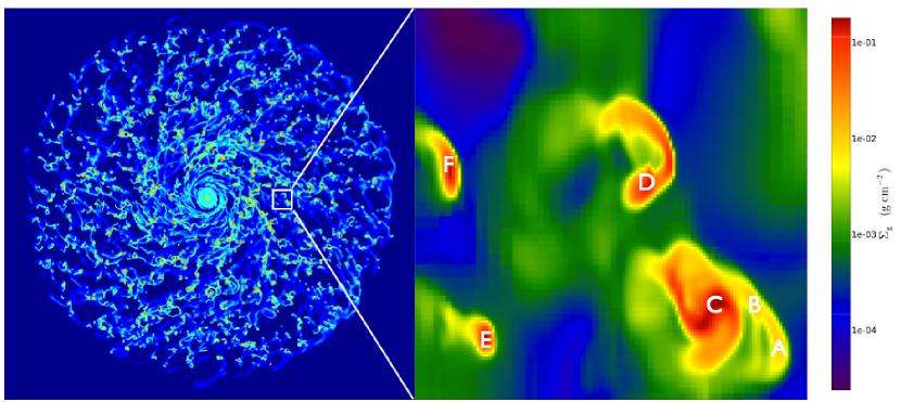
Figure 1.— View of the gas mass surface density, $\Sigma_{g}$, over the 20 kpc diameter galactic disk of TT09 250 Myr after start of the simulation. The square is a 1 kpc sided region, enlarged in the right image, showing several GMCs. These are the initial conditions for the simulations of this paper. The intial clouds listed in Table 3 are marked.

Our approach is to extract a 1 kpc by 1 kpc patch of the disk, extending 1 kpc both above and below the midplane, centered at a radial distance of 4.25 kpc from the galactic center (see Fig. 1). This is done at a time 250 Myr after the beginning of the TT09 simulation, when the disk has fragmented into a relatively stable population of GMCs. We then follow the evolution of the ISM, especially the GMCs, including their interactions, internal dynamics and star formation activity, down to $\lesssim$ parsec scales. These local simulations are able to reach higher densities, resolve smaller mass scales and include extra physics compared to the global simulations.

Setting up the local simulations requires performing a velocity transformation to remove the circular velocity at each location and then adding a shearing velocity field so that the reference frame of the simulation is the local standard of rest at the center of the extracted patch of the galaxy disk. Periodic boundary conditions are introduced for the box faces perpendicular to the shear flow (along the $y$-axis) and outflow boundary conditions for the other faces. This set up is similar to shearing box simulations of astrophysical disks, but does not include the rotation of the frame of the patch (thus neglecting Coriolis forces). Since we only consider the evolution of the ISM over quite short timescales $\sim 10$ Myr (which is several local dynamical times of the GMCs, but much shorter than the orbital time of $130$ Myr), this approximation should not have a significant effect on the properties of the clouds and their star formation activity.

We also ignore radial gradients in the galactic potential, only including resulting forces perpendicular to the disk. The model for the potential is that used by TT09, i.e. Binney & Tremaine (1987), evaluated at $r=4.25$ kpc:

$$\Phi=\frac{1}{2}v_{c,0}^{2}\ln\left[\frac{1}{r_{c}^{2}}\left(r_{c}^{2}+r^{2}+\frac{z^{2}}{q_{\phi}^{2}}\right)\right],$$ (1)

where $v_{c,0}$ is the constant circular velocity in the limit of large radii, here set equal to $200\>{\rm km\>s^{-1}}$, $r_{c}$ is the core radius set to 0.5 kpc, $r$ and $z$ are the radial and vertical coordinates respectively, and the axial ratio of the potential field is $q_{\phi}=0.7$.

The grid resolution of the initial conditions is 128${}^{2}\times$ 256 which corresponds to a cell size of 7.8 pc and serves as the root grid for the high resolution simulations. Most of the simulations we present here involve 4 levels of adaptive mesh refinement of the root grid, thus increasing the effective resolution to 2048${}^{2}\times 4096$ or about 0.5 pc. Refinement of a cell occurs when the Jeans length drops below four cell widths, in accordance with the criteria suggested by Truelove et al. (1997) for resolving gravitational instabilities.

The simulations performed in this paper were run using Enzo (Bryan & Norman, 1997; Bryan, 1999; O’Shea et al., 2004). We use the second order Godunov scheme with the Local Lax-Friedrichs (LLF) solver and a piecewise-linear reconstruction to evolve the gas equations. Because gas temperatures calculated from the total energy can become negative when the total energy is dominated by the kinetic energy, we also solve the non-conservative internal energy equation. We use the gas temperature value from the internal energy when the internal energy is less than one tenth of the total energy and from the total energy otherwise. While this is higher than the often adopted ratio of 10^-3, it does not affect the dynamics.

Table 1Star Particle Creation.

Cell Size	$n_{\rm H,sf}$	$t_{\rm ff}$	Min. Cell Mass	$M_{\rm*,min}$
(pc)	(${\rm cm^{-3}}$)	(yr)	($M_{\odot}$)	($M_{\odot}$)
7.8	100	$4.3\times 10^{6}$	1640	1000a
0.49	$10^{5}$	$1.4\times 10^{5}$	400	100
0.125	$10^{6}$	$4.3\times 10^{4}$	63	10b

^a Used in test runs not presented here and by Tasker (2011)
^b Used in runs to be presented by Butler, Van Loo & Tan, in prep.

2.2. Star Formation

To model star formation, we allow collisionless star cluster particles, i.e. a point mass representing a star cluster or sub-cluster of mass $M_{*}$, to form in our simulations. These star cluster particles are created when the density within a cell exceeds a fiducial star formation threshold value of $n_{\rm H,sf}=10^{5}$ cm^-3 for our 4-level refinement runs compared to a threshold of 10² cm^-3 in the lower resolution simulation of Tasker (2011). (Note we assume $n_{\rm He}=0.1n_{\rm H}$ so that the mass per H is $2.34\times 10^{-24}\>{\rm g}$). This density threshold is a free-parameter of our modeling, and its choice depends on the minimum mass that is allowed for star particles and the minimum cell resolution (see Table 1).

We use a prescription of a fixed star formation efficiency per local free-fall time, $\epsilon_{\rm ff}$, for those regions with $n_{\rm H}>n_{\rm H,sf}$. Relatively low and density-independent values of $\epsilon_{\rm ff}$ are implied by observational studies of GMCs (Zuckerman & Evans, 1974) and their star-forming clumps (Krumholz & Tan, 2007), which motivate our fiducial choice of $\epsilon_{\rm ff}=0.02$. Such values are also approximately consistent with numerical studies of turbulent, self-gravitating gas (Krumholz & McKee, 2005) and turbulent, self-gravitating, magnetized gas (Padoan & Nordlund, 2011). Note that given the inability of our simulations to resolve individual star-forming cores, we do not impose requirements that the gas flow be converging or that the gas structure be gravitationally bound in order for star formation to proceed. However, to rule out the possibility of star formation in the hot dense gas of shock fronts, cells with temperatures greater than 3000 K are prevented from forming stars. In fact, such conditions almost never arise in the simulations presented here.

When a cell reaches the threshold density, a star cluster particle is created whose mass is calculated by

$$M_{*}=\epsilon_{\rm ff}\frac{\rho\Delta x^{3}}{t_{\rm ff}}\Delta t,$$ (2)

where $\rho$ is the gas density, $\Delta x^{3}$ the cell volume, $\Delta t$ the numerical time step, and $t_{\rm ff}$ the free-fall time of gas in the cell (evaluated as $t_{\rm ff}=(3\pi/32G\rho)^{1/2}$).

An additional computational requirement is the minimum star cluster particle mass, $M_{\rm*,min}$, introduced to prevent the calculation from becoming prohibitively slow due to an extremely large number of low-mass particles. If the calculated $M_{*}$ is $<M_{\rm*,min}$ then a star cluster particle of mass $M_{\rm*,min}$ is created with probability $M_{*}/M_{\rm*,min}$. In fact given the low value of $\epsilon_{\rm ff}$, the fact that $\Delta t\ll t_{\rm ff}$ and our adopted values of $M_{\rm*,min}$, we are always in this regime of “stochastic star formation”.

The motions of the star cluster particles are calculated as a collisionless N-body system. Note these are not sink particles: there is no gain of mass by gas accretion. They interact gravitationally with the gas via a cloud-in-cell mapping of their positions onto the grid to produce a discretized density field. Note, however, that gravitational interactions between star cluster particles are thus softened to the resolution of the grid. In reality the distribution of stellar mass represented by the star cluster particle would be spread out, but by amounts that are not set by the local gas density. Thus the structure of star clusters, made up of many simulation star cluster particles, is not well-modeled in our simulations and we do not present results on the details of the star clusters that form.

2.3. Thermal processes

To describe the thermal behaviour of the ISM, we include a net heating rate per unit volume given by

$$H=n_{\rm H}[\Gamma-n_{\rm H}\Lambda]\ {\rm erg\ cm^{-3}\ s^{-1}},$$ (3)

where $\Gamma$ is the heating rate and $\Lambda$ the cooling rate. Below we describe several different methods to model heating and cooling.

The thermal processes introduce a new time scale, i.e. the cooling time $t_{\rm cool}\equiv E_{\rm int}/|H|$ where $E_{\rm int}=p_{g}/(\gamma-1)$ is the internal energy, which is often much shorter than the dynamical time step set by the Courant condition. To prevent the cooling from increasing the numerical cost significantly, we set the numerical time step to the hydrodynamical time step and sub-cycle the cooling with smaller time steps, i.e. $0.1t_{\rm cool}$ until the total cooling time step equals the dynamical time step.Then the temperature and internal energy are updated explicitly every sub-cycle after which the net heating rate and cooling time are recalculated. This sub-cycling prevents overcooling and negative pressures by not resolving the cooling time. If the hydrodynamical time step is shorter than the cooling time, no sub-cycling is necessary.

2.3.1 Simple Photoelectric Heating

FUV radiation is absorbed by dust grains causing electrons to be discharged, which then heat the gas. This photoelectric (PE) heating has long been thought to be the dominant heating mechanism in the neutral ISM, including the relatively low extinction portions of GMCs (Wolfire et al., 1995). We include a PE heating term

$$\Gamma_{\rm PE}=1.3\times 10^{-24}\epsilon G_{0}\ \ {\rm erg\ s^{-1}},$$ (4)

where $\epsilon$ is the heating efficiency and $G_{0}$ the incident FUV field normalized to the Habing (1968) estimate for the local ISM value. We set the heating efficiency to its maximum value of $\epsilon=$0.05 for neutral grains (Bakes & Tielens, 1994). Also, we adopt $G_{0}=4$ as a value appropriate for the radial location of the simulated region in a Milky Way-type galaxy, in agreement with Wolfire et al. (2003). Note that this estimated heating rate is approximate in the sense that it does not follow the attenuation of the FUV field in the dense gas, nor its local generation from young star clusters.

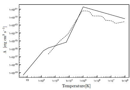
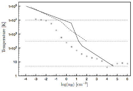
Figure 2.— Left: Cooling rate as function of temperature as defined by Sanchez-Salcedo et al. (2002) (solid) and Rosen & Bregman with the high temperature range ($>10^{5}$ K) from Sarazin & White (1987) (dashed). Right: The equilibrium temperatures for the Rosen & Bregman (dashed) and Sanchez-Salcedo et al. (solid) cooling curves assuming a constant PE heating term with $G_{0}=4$ and for the Cloudy heating and cooling rates (squares). The dashed lines represent lines of constant temperature at 10⁴, 300 and 5 K.

2.3.2 Simple Atomic Cooling

We consider several cooling functions. Initially and for the higher temperature regime, we adopt the solar metallicity cooling curve of Sarazin & White (1987) from temperatures of $T=10^{8}$ K down to $T=10^{5}$ K (although we do not expect gas temperatures in our simulations to exceed a few times $10^{6}$ K) and extend it down to $T=300$ K using rates from Rosen & Bregman (1995) (see Fig. 2). These temperatures take us to the upper end of the atomic cold neutral medium (Wolfire et al., 1995). This cooling function is similar to that used by TT09. The floor temperature of 300 K acts as a minimum of thermal support against gravitational collapse and fragmentation. It imposes a minimum signal speed equal to the sound speed $c_{s}=(\gamma kT/\mu m_{p})^{1/2}\approx 1.80(T/300{\rm K})^{1/2}\ {\rm km\ s^{-1}}$, where $\gamma=5/3$ and $\mu=1.27$ (for an assumed $n_{\rm He}=0.1n_{\rm H}$). This signal speed is of the same order as observed velocity dispersions of clumps within GMCs (e.g. Barnes et al., 2011).

Figure 3.— Mean logarithmic visual extinction as a function of the density as derived using the Sanchez-Salcedo et al. simulation. The error bars show the dispersion on the mean, while the shaded area shows the distribution of all column extinctions in the numerical domain. The solid line represents the minimum column extinction due to absorption within the cell itself (see Eq. 6).

However, the Rosen & Bregman cooling function does not include the formation and destruction of molecules or any cooling processes below the minimum temperature of 300 K. By a combination of dust cooling and atomic and molecular line cooling, gas in real GMCs reaches temperatures of $\sim 5-10$ K. We first take into account the effect of dust grains by adopting the atomic cooling function of Sanchez-Salcedo et al. (2002), which mimics the equilibrium phase curve of Wolfire et al. (1995). Figure  2 shows the difference between the Sanchez-Salcedo et al. and the Rosen & Bregman cooling rates. Note that, while the cooling rates are roughly the same for both curves, the Sanchez-Salcedo et al. cooling curve extends down to 5 K and has a thermally unstable temperature range between 313-6102 K. This gives rise to the co-existence of a cold and warm phase at the same pressure.

2.3.3 Extinction-Dependent Heating and Cooling Functions

A density-column extinction relation

The inclusion of molecular cooling is less straightforward since the formation of molecules depends strongly on the amount of attenuation of the radiation field. Molecules only form in the regions of relatively dense gas and dust that can shield their contents from destructive UV radiation. This means that the molecular cooling rate, and also heating rate, depends not only on density and temperature, but also on column extinction.

Of these three variables, the column extinction is the only one that is not directly available during the simulation. For every grid cell an effective column extinction due to dust absorption can be calculated using a six-ray approximation (e.g. Glover & Mac-Low, 2007). Using the linear relation between column density and visual extinction, i.e. $A_{V}=5.35\times 10^{-22}N_{\rm H}$, the effective visual extinction is given by (Glover & Mac-Low, 2007)

$$A_{V,{\rm eff}}=-\frac{1}{2.5}\log\left[\frac{1}{6}\sum_{i=1}^{6}{\exp(-2.5A_{V,i})}\right]{\rm mag}.$$ (5)

Although the six-ray approximation already reduces the numerical cost of calculating the column extinction considerably, it remains time-consuming as it needs to be calculated for every cell at every time step. Still, an additional simplification can be made. In general, higher density gas has a higher column extinction than the surrounding lower density gas. We calculate the effective column extinction for the high-resolution run with the Sanchez-Salcedo et al. cooling function (see Sect. 3.4) at 10 Myr, but neglect cells within 10 grid spacings of the computational boundary. Figure 3 shows the full range of column extinctions in the numerical domain, i.e. the shaded area, and the mean logarithmic column extinction as a function of the density with the error bars indicating the dispersion on the mean. We omitted density bins with fewer than ten cells contributing to the mean. While the extrema of the column extinction differ by more than an order of magnitude (similar to the results of e.g. Clark et al., 2012), the dispersion on the mean is much smaller. For example, at $n_{\rm H}=10\ {\rm cm^{-3}}$, 95% of all visual extinctions lie within the $0.458\pm 0.021$ interval. Thus, the mean value is representative for the column extinction at a given density. An a posteriori check on the simulations using this relation (i.e. Run 5, 6 and 7 of Table 2) shows little deviation from the above result.

The sudden increase at $n_{\rm H}\approx 10^{4}{\rm cm^{-3}}$ is due to the resolution limitation, i.e. the effective visual extinction is dominated by absorption within the cell itself, i.e.

$$A_{V,{\rm eff}}=5.35\times 10^{-22}\frac{\Delta x}{2}n_{\rm H}~{}{\rm mag},$$ (6)

or $A_{V,{\rm eff}}=4.1~{}{\rm mag}$ for $n_{\rm H}=10^{4}~{}{\rm cm^{-3}}$ and $\Delta x$ = 0.5 pc. The high density end is thus resolution-dependent and the column extinction is most likely overestimated. However, for $A_{\rm V}>10$, the heating rate (and ionization balance) is dominated by cosmic rays (see later), so this limitation should not affect the cooling and heating rates significantly.

A table of heating and cooling rates

Using the density-column extinction relation we now generate a table of cooling and heating rates as function of density and temperature using the photodissociation code Cloudy (Ferland et al., 1998, version c08.01). The routine is similar to the one of Smith et al. (2008) and goes as follows. Firstly, for a given density, ranging from 10^-3 to 10⁶ cm^-3 with steps of 1 dex, the unextinguished local interstellar radiation field (Black, 1987) with $G_{0}=4$ is directed through an absorbing slab. This slab has a constant density of $n_{\rm H}=1{\rm cm}^{-3}$, similar to the mean density of the disk in the initial conditions and a thickness corresponding to the visual extinction at the given density (see Fig. 3). We assume the gas has solar abundances and include a dust grain population with PAHs. The dust grain physics used in the code is described in van Hoof et al. (2004) and Weingartner et al. (2006). Background cosmic rays are also included with a primary ionization rate of 2.5$\times 10^{-17}\ {\rm s}^{-1}$, as well as the cosmic background radiation.

The transmitted continuum, i.e. the sum of the attenuated incident and diffuse continua and lines, is then used as the radiation field incident on a gas parcel with the given density. The resulting cooling and heating rates, for a range of temperatures between 5 and 10⁵ K, are calculated self-consistently by simultaneously solving for statistical and ionization equilibrium including all the necessary microphysics such as, among others, H₂ and CO formation and destruction. For temperatures above 10⁵ K we opt not to use Cloudy and simply adopt the cooling curve of Sarazin & White (1987) and set the heating rate to zero. From the generated table, the heating and cooling rates for any density and temperature are derived using a bilinear interpolation. For densities and temperatures above and below the table limits, the rate of the limiting value is used. We implemented such a heating and cooling routine into Enzo.

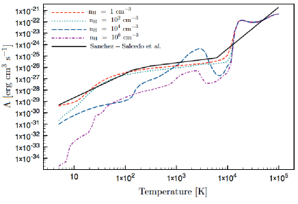
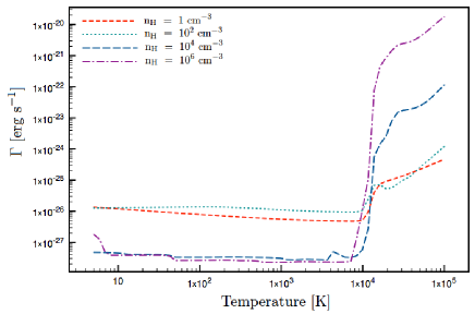
Figure 4.— The cooling (left) and heating (right) rates as function of temperature for densities of 10⁰ (short-dashed), 10² (dotted), 10⁴ cm^-3 (long-dashed) and 10⁶ cm^-3 (dash-dotted) calculated using Cloudy. The cooling rates of Sanchez-Salcedo et al. (solid) are also plotted as reference.

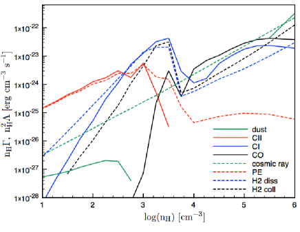
Figure 5.— Cooling (solid) and heating (dashed) rates per unit volume as function of density for the Cloudy cooling function equilibrium temperatures given in Fig. 2. Only the processes that contribute the most are shown.

Figure 4 shows the calculated heating and cooling rates as a function of temperature for selected densities. The Sanchez-Salcedo et al. cooling curve is also plotted showing a close similarity in shape and magnitude for densities up to $\sim 10^{2}$ cm^-3. The deviation from the Sanchez-Salcedo et al. curve at higher densities stems from the onset of molecular cooling. Molecules form in regions with visual extinctions higher than $A_{V}=2.4$ or column extinctions higher than 4.3 $\times 10^{21}$ cm^-2 (e.g. Tielens & Hollenbach, 1985). Using the derived density-column extinction relation this translates to densities above $\approx 10^{3}~{}{\rm cm^{-3}}$. Figure 5 shows the decomposition of the heating and cooling rates at thermal equilibrium (see Fig. 2 for the equilibrium temperatures). From this figure, we indeed find that molecular species, i.e. H₂ and CO, contribute significantly to the heating and cooling above 10³ cm^-3. Note that this figure is very similar to Fig. 8 of Glover & Clark (2012) in both the decomposition and the level of cooling rates. Note also that, the dust cooling disappears between $\approx 10^{3}-10^{5}$ cm^-3. Up to 10⁵ cm^-3, the dust grains are hotter than the gas. In these conditions, ion-grain collisions heat the gas due to thermal evaporation of neutralized ions (see Eq. 32 of Baldwin et al. (1991)), while electron-grain collisions cool the gas. At densities below 10³ cm^-3 the electron-grain collisions dominate the ion-grain collisions so that the net effect is gas cooling. As the density (and extinction) increases, less ionizing radiation can penetrate the gas. Then ion-grain collisions start to dominate the electron-grain collisions and, consequently, the gas is heated. Above 10⁵ cm^-3 the dust temperature falls below the gas temperature and grain collisions result in cooling of the gas.

While the Cloudy cooling rates are adequately described by the Sanchez-Salcedo cooling function (up to 10² cm^-3), the Cloudy heating rates deviate significantly from the PE heating rate we use with the atomic cooling functions, i.e. $\approx 2.6\times 10^{-25}$ erg s^-1. It is clear that we have overestimated the heating efficiency by approximately an order of magnitude. At high densities, the PE heating is no longer the dominant heating process (see Fig. 5). Higher density regions tend to have higher dust extinctions of the external radiation field, thus blocking FUV penetration and PE heating. Then only cosmic rays can penetrate and heat the gas. The overall heating rate is further reduced by an order of magnitude.

Not only does the decomposition of the cooling and heating rates give useful insights into the dominant processes at different temperatures and densities, it also provides the opportunity to compare the numerical simulations with observations. For different emission lines, such as the 158 $\mu$m CII line and the 63 $\mu$m OI, tables similar to the cooling and heating rate tables can be constructed. Then emissivity maps and line profiles of optically-thin emission lines can be generated from the simulations during post-processing. Note, however, that such emission maps are only first order approximations as they do not include any radiative transfer, nor do they take into account the effects of time-dependent chemistry (e.g. Glover & Mac-Low, 2007, 2011) or local abundance variations (Shetty et al., 2011a, b).

Thermal instability?

Although the Cloudy cooling curve (for $n_{\rm H}<10^{2}$ cm^-3) has a similar temperature dependence between 300-6000 K as the Sanchez-Salcedo et al. curve, the equilibrium curve only exhibits a weak thermal instability (see Fig. 2). Furthermore, the instability is at lower densities than the Sanchez-Salcedo et al. curve. The shift of the instability towards lower densities is due to a higher column extinction compared to the 10¹⁹ cm^-2 used by Wolfire et al. (1995). At low densities, the thermal equilibrium is set by the Ly$\alpha$ cooling and PE heating. The increased attenuation reduces the electron fraction in the gas resulting in a lower PE heating (and thus a lower equilibrium temperature).

Once the equilibrium temperature drops below 10⁴ K (and this happens at lower densities), CII cooling becomes the dominant cooling process. Wolfire et al. (1995) show that the thermal instability can be attributed to CII cooling which causes a rapid drop in equilibrium temperature. The magnitude and presence of the thermal instability then depends on the temperature and density dependence of the CII cooling. Interstellar gas is thermally unstable if (Field, 1965)

$$\frac{n_{\rm H}}{T}\left(\frac{\partial H}{\partial n_{\rm H}}\right)_{T}-\left(\frac{\partial H}{\partial T}\right)_{n_{\rm H}}<0.$$ (7)

By expressing the heating and cooling rate locally as a power-law of density and temperature, the instability constraint reduces to

$$(a-b)-(\alpha-\beta)<1,$$ (8)

where $a$, resp. $b$, is the density, resp. temperature, power-law index for the heating rate and $\alpha$ and $\beta$ the indices for the cooling rate. We can use the above constraint to understand the weak instability seen in Fig. 2. For temperatures between $300-6000$ K the cooling rate has a power-law index of the order of 0.5, while the heating rate shows no temperature dependence, i.e. $\beta\approx 0.5$ and $b\approx 0$ (see Fig. 4). Similarly, while the heating rate index, $a$, is roughly zero between 0.1 and 1 cm^-3 (the range of densities for which the equilibrium temperatures is between 300 and 6000 K), the cooling rate decreases roughly as $n_{\rm H}^{-0.5}$. As a result, $(a-b)-(\alpha-\beta)\approx 1$. The instability criterion is thus only marginally satisfied explaining the weak thermal instability.

Table 2Set of simulations.

Run	AMRa	Heating	Cooling	$\mu$	Star formation
1	No	No	RBb	1.27	No
2	Yes	No	RB	1.27	No
3	Yes	PE	RB	1.27	No
4	Yes	PE	SSc	1.27	No
5	Yes	Cloudy	Cloudy	1.27	No
6	Yes	Cloudy	Cloudy	2.33	No
7	Yes	Cloudy	Cloudy	2.33	Yes

^a “No” implies min. resolution of $8$ pc; “Yes” implies min. resolution of 0.5 pc
^b Rosen & Bregman cooling function
^c Sanchez-Salcedo et al. cooling function
^d Photoelectric heating

3. Results

To understand the effect of different physical processes, we gradually include them in our models. All the details (e.g. included physics) of the simulations that we ran are listed in Table 2.

3.1. Measures of ISM Structure

Several methods can be used to compare the different simulations and quantify the effect of the included physical processes. We focus on measures that describe the changes in density and temperature.

A visual analysis of the simulations is the simplest and quickest method of studying the geometrical changes. Column density plots show how the density structures change over time, with the maximum/minimum values indicative of increases/decreases in the density.

We also follow the evolution of the mass fraction of the gas that is in defined density ranges: “GMC” gas is defined by $n_{\rm H}>10^{2}$ cm^-3 and “Clump” gas is defined by $n_{\rm H}>10^{5}$ cm^-3. Using our density-column extinction relation, this corresponds to a mean $A_{V,\rm eff}>0.7$ for GMC gas and $A_{V,\rm eff}>40$ for clump gas. While a visual extinction of 0.7 does not imply molecular gas, it is only above $n_{\rm H}=10^{2}{\rm cm^{-3}}$ that we find gas with $A_{V,{\rm eff}}>2.4$ (see Fig. 3). The density and column density structure can also be studied in more detail by using mass weighted probability density functions at different times.

As the ISM has different phases, we also examine the mass fractions of the different temperature regimes, i.e. the cold, unstable, warm and hot phases. For the cold phase, $T<350$ K. The unstable phase lies within the range of 350-6000 K. The warm phase extends from 6000 to 10⁵ K after which the hot phase starts. These values are only indicative and we can even argue whether we need to include a thermally unstable range. Technically the Rosen & Bregman cooling function does not have one and the thermal instability in the Cloudy cooling function is weak.

Finally, we also use a clump-finding routine (Smith et al., 2009, for details) to identify individual molecular clouds and derive their properties such as their mass, velocity dispersion and size. For this purpose, we adapted the clump-finding routine included in YT (Turk et al., 2011). This routine can also be used to identify dense clumps within the molecular clouds. However, as the highest resolution in our simulations is only 0.5 pc, clumps with sizes of the order of 1 pc are not properly resolved. Therefore, we refrain from any detailed analysis of the clumps.

Table 3List of the initial GMCs.

Cloud	Mass center	Mass	$\sigma^{a}$	Rb	$\alpha_{\rm vir}^{c}$
	position (x,y,z)	(106 M⊙)	(km s-1)	(pc)
A	0.921, 0.164, -0.004	0.09	3.6	17.9	1.70
B	0.865, 0.249, 0.004	0.06	2.5	15.1	1.50
C	0.745, 0.232, 0.013	7.47	15.4	47.9	0.61
D	0.605, 0.597, 0.005	2.53	16.1	37.4	1.54
E	0.180, 0.159, -0.003	0.79	10.5	21.5	1.26
F	0.089, 0.588, -0.003	1.00	10.8	27.0	1.32

^a $\sigma$ is the mass-weighted three-dimensional velocity dispersion.
^b The radius is calculated from the cloud’s volume assuming a spherical geometry.
^c The virial parameter is calculated as $\alpha_{\rm vir}=\frac{5\sigma_{c}^{2}R}{GM}$, where $\sigma_{c}$ is the one-dimensional velocity dispersion inside the cloud and given by $\sigma_{c}^{2}=\frac{\sigma^{2}}{3}+c^{2}_{s}$ (Dib et al., 2007).

3.2. Initial Conditions

Figure 1 shows the column density integrated along the $z$-axis and we can identify four distinct density structures. In fact, the selected region contains six clouds. The two small clouds (A & B) are about to interact with a larger one (C) and are therefore not recognized as individual clouds in the column density plot. Table 3 lists all of the clouds. Their properties span a large range in sizes and masses. The smallest cloud only has a radius of 15 pc and a mass of 6$\times 10^{4}M_{\odot}$, while the largest cloud is a hundred times more massive ($7.47\times 10^{6}M_{\odot}$) and 30 times larger in volume. The total mass in the clouds is 1.2$\times 10^{7}M_{\odot}$ which is about 70% of the gas mass in the simulation box. The clouds have diameters smaller than $\sim$ 100 pc, and thus have at most $\sim 12$ cells ($\Delta x\approx 7.8$ pc) across each linear dimension. To resolve turbulence in self-gravitating gas, Federrath et al. (2011) suggest that the turbulent length-scale needs to be resolved by at least 30 grid cells. The internal structure of the clouds and their internal turbulence is thus not resolved in the initial conditions. Note, however, that the velocity dispersion of the clouds is significantly larger than the minimum sound speed of 1.8 km s^-1 and increases with the cloud radius. Actually, the initial velocity dispersion of the clouds is high enough to give some approximate balance against self-gravity. The mean virial parameter of the clouds is 1.32 with standard deviation of 0.35, close to the value of 1.3 with standard deviation of 0.76 for Galactic GMCs derived by McKee & Tan (2003) from analysis of the results of Solomon et al. (1987). Note the $\rm{}^{13}CO$-selected clouds studied by Roman-Duval et al. (2010), which trace somewhat higher densities, have median virial parameters of 0.46. The values listed here are also in agreement with the values from the simulations of Dobbs et al. (2011).

The temperature distribution of the initial conditions shows that 99% of the mass has a temperature below 350 K and is therefore in the cold phase. All this gas lies within the galactic disk. The remaining 1% of the mass is diffuse hot gas with temperatures above 10⁵ K surrounding the disk. TT09 were not studying the full temperature structure of the warm gas and so did not yet include a heating term in their simulations. Thus most of the gas cooled down to the minimum temperature of 300 K, with hotter components created in shocks. The cooling time for low density gas with temperatures above 10⁵ K (i.e. the gas outside the disk) is of the order of 10⁴ Myr and, thus, remains hot. As the hot gas lies outside the disk, its volume fraction can be used to derive a mean thickness of the disk, i.e. 140 pc.

3.3. Evolution of Structure and Effect of Resolution

We first carryout the simulation, running for 10 Myr, with the physics and resolution identical to the global galaxy simulation of TT09.

For the given resolution of $\sim$ 7.8 pc and the minimum temperature of 300 K, the Truelove et al. (1997) criterion, i.e. the Jeans length, $\lambda_{J}=(\pi c_{s}^{2}/G\rho)^{1/2}$ where $G$ is the gravitational constant, associated with a grid cell should be at least 4 times larger than the size of the cell, $\Delta x$, is satisfied for densities up to $n_{\rm H}\simeq 80\>{\rm cm^{-3}}$. Similar considerations for the higher resolution simulations that include cooling down to $\sim 5$ K and reach much higher densities indicate that the Truelove criterion is not satisfied for resolving clump formation within GMCs. Artificial fragmentation is expected to happen above densities of 5$\times 10^{2}$, 1.5$\times 10^{3}$ and 2$\times 10^{4}$ cm^-3 for the Cloudy, Sanchez-Salcedo et al. and Rosen & Bregman cooling functions, respectively.

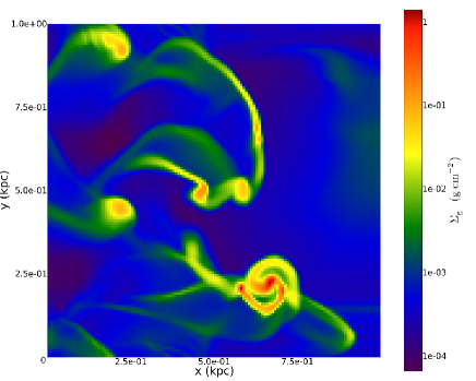
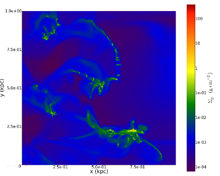
Figure 6.— Gas mass surface density along the $z$-axis after 10 Myr for the uniform Run 1 (left) and the AMR Run 2 (right).

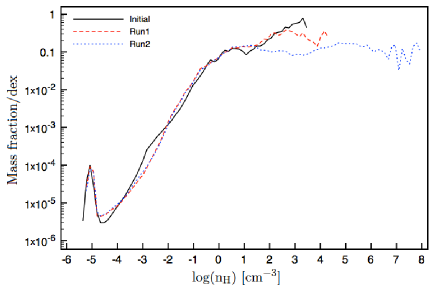
Figure 7.— Mass-weighted Probability Density Function (PDF) for Run 1 (red, dashed) and Run 2 (blue, dotted) after 10 Myr. We also plot the initial PDF (solid line).

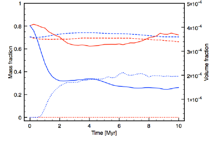
Figure 8.— The mass fraction of gas in “GMCs” ($n_{\rm H}>10^{2}{\rm cm^{-3}}$; dashed) and in “Clumps” ($n_{\rm H}>10^{5}{\rm cm^{-3}}$; dotted) and the volume fraction of gas in “GMCs” (solid) for Run 1 (red) and Run 2 (blue).

Table 4List of GMCs after 10 Myr for Run 1 and 2.

Cloud	Mass	$\sigma$	R	$\alpha_{\rm vir}$
Run 1	(106 M⊙)	(km s-1)	(pc)
Aa	-	-	-	-
Ba	-	-	-	-
C	7.7	17.7	44.7	1.04
D1b	0.41	5.1	22.3	1.10
D2b	0.51	4.8	25.5	0.73
D3b	0.87	6.9	25.3	0.92
E	0.70	5.5	26.1	0.81
F	0.76	6.7	27.6	0.99

Cloud	Mass	$\sigma$	R	$\alpha_{\rm vir}$
Run 2	(106 M⊙)	(km s-1)	(pc)
Aa	-	-	-	-
Ba	-	-	-	-
C1b	1.1	13.6	21.9	2.2
C2b	6.9	25.6	29.0	4.1
D1b	0.10	6.4	9.3	3.1
D2b	0.12	5.5	10.2	2.0
D3b	0.48	16.4	12.3	5.4
D4b	0.12	14.8	18.0	1.9
D5b	0.19	13.0	6.4	4.5
D6b	0.11	8.4	6.4	2.9
E	0.70	15.2	14.7	2.9
F1b	0.16	6.8	9.6	1.6
F2b	0.81	12.4	15.4	2.0

^a Cloud A and B merge with cloud C.
^b The cloud fragments into multiple clouds.

Figure 6 shows the gas surface density for Run 1 (left panel) after 10 Myr. The clouds have not changed dramatically over this time scale, but do show signs of gravitational contraction, interaction (e.g. clouds A & B merge and collide with cloud C) and fragmentation (e.g. cloud D). The result of these interactions can be seen in the mass weighted PDFs (Fig. 7), i.e. the “GMC” gas is redistributed over a slightly larger density range. However, the same PDF also shows that the mass fraction of gas in “GMCs” is roughly the same as initially. In fact, the fraction remains quite constant throughout the simulation, which spans a few free-fall times (Fig. 8). The volume fraction of “GMC” gas shows an initial decrease, but also remains relatively constant. Thus the clouds are roughly in virial equilibrium as indicated by their initial and final virial parameters (see Tables 3 and 4). Thermal pressure and non-thermal motions within the clouds thus provide enough support against self-gravity to prevent runaway gravitational collapse (even though the non-thermal motions are not well resolved in this uniform grid simulation). A similar observation was made by TT09 in their global simulation, i.e. the gas properties in the full disk are quasi-steady after timescales of about 150 Myr. However, note that now the velocity frame of the simulation volume is the local standard of rest of the disk at the center of the box, so the fast, $\sim 200\>{\rm km\>s^{-1}}$ orbital velocities that were present in the TT09 simulation are now absent. Modeling these fast circular velocities on a finite rectilinear grid led to relatively large numerical viscous heating that helped stabilize the TT09 GMCs. Thus it is not surprising that we now see that the clouds are able to evolve to somewhat higher densities than were seen by TT09.

By increasing the resolution up to $\sim 0.5$ pc the GMCs can now be better resolved and the evolution of dense clumps within the clouds begins to be captured. While the “GMC” mass fraction increases slightly to 72%, the volume fraction decreases by a factor of 2 within 2 Myr after which it remains roughly constant (see Fig. 8). In approximately the same time span, about half of the “GMC” gas accumulates in “Clumps” (see Fig. 8). Then the mass fraction in clumps remains nearly constant and reaches a new quasi-steady state. So, initially, the gas within the clouds collapses to form filaments with dense clumps due to the increased resolution. The clouds thus contract, but, at the same time, the velocity dispersion in the clouds increases. Thermal pressure and non-thermal motions again counter the effects of self-gravity to virialize the cloud (the virial parameters of the clouds are given in Table 4). The initial evolution of the clouds is thus a direct consequence of the increase in resolution.

The formation of clumps can also be seen in the PDFs (see Fig. 7). While the PDFs for Run 1 and 2 are similar up to $n_{\rm H}=80~{}{\rm cm}^{-3}$, the gas above the “GMC” density threshold is redistributed towards higher densities. The higher densities also give rise to higher surface densities, i.e. the maximum value increases to $\sim 10^{2}~{}{\rm g~{}cm^{-2}}$ (see Fig. 6).

3.4. A Multiphase Interstellar Medium

While the increased resolution helps to describe the substructures of GMCs in greater detail, the thermal properties of the ISM are poorly reproduced. As only cooling is included in Run 1 and 2, most of the gas within the disk is at the floor temperature of 300 K. To reproduce the multiphase character of the ISM, i.e. a cold, dense and a warm, diffuse phase, we include diffuse heating. Additionally, we study the influence of different cooling functions. While atomic cooling can be adequately described by the Rosen & Bregman cooling function (used in Sect. 3.3), the Sanchez-Salcedo et al. function extends down to a temperature of 5 K, i.e. nearly two orders of magnitude lower, and includes a thermally unstable temperature range. Extinction-dependent cooling, especially from CO molecules, is only taken into account in the Cloudy cooling function.

Including diffuse heating mostly affects the gas outside the GMCs. Figure 2 shows that, for $n_{\rm H}<90$ cm^-3, the gas has a higher equilibrium temperature than 300 K. For the other cooling functions the critical density for heating is at lower densities, i.e. 10 cm^-3 for Sanchez-Salcedo et al. and 1 cm^-3 for Cloudy. The diffuse intercloud gas thus moves from the cold phase to the warm phase. The decrease in the cold gas mass fraction is most significant for the Rosen & Bregman cooling function. Only the “GMC” gas which is 70% of the total, remains in the cold phase. For the Sanchez-Salcedo et al., resp. Cloudy, cooling function, some of the gas surrounding the clouds is also in the cold phase so that the mass fractions are 85%, resp. 96%. The mass fraction of gas that is in the cold phase (i.e. molecular gas and CNM) in the inner Galaxy disk region of the molecular ring is $\sim 0.5$ (Wolfire et al. 2003). The simulation values for this mass fraction are somewhat higher, which we expect is due mostly to their present lack of ionization and supernova feedback processes.

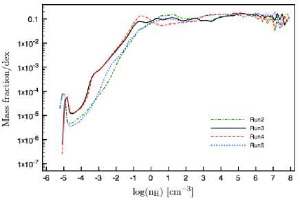
Figure 9.— Same as Fig. 7, but for Run 2 (green, dash-dotted), Run 3 (solid), Run 4 (red, dashed) and Run 5 (blue, dotted).

Together with the temperature, the pressure in the intercloud region increases significantly. For example, for $n_{\rm H}=1$ cm^-3, the pressure difference is of the order 10${}^{4}k_{B}$, where $k_{B}$ is the Boltzmann constant. The associated heating time scales are of the order of 0.1 Myr for 0.1 cm^-3, but are much shorter and even below the numerical time step for $n_{\rm H}>1$ cm^-3. (Remember that the time step is determined by the Courant condition for the hydrodynamics and not limited by the cooling time.) As a consequence, a significant amount of energy is added during the first time step to the simulation, i.e. of the order of 10⁵⁰ erg for the Rosen & Bregman and the Sanchez-Salcedo et al. functions and 10⁴⁸ erg for the Cloudy function. Note that this initial adjustment is unphysical, and can be regarded as a transient associated with the initial conditions. The added energy is primarily deposited near the midplane of the disk and eventually causes the disk to expand. The mean disk thickness for Run 3 and Run 4 (the atomic cooling functions) is $\sim$ 600 pc, an increase of a factor of 4, after 10 Myr. Because of the lower energy deposit for the Cloudy function, the mean disk thickness of Run 5 increases only by 30% to 190 pc. The larger disk of Run 3 and 4 can also be seen in Fig. 9 where the PDFs show that the densities between 10^-4 and 1 cm^-3 contain more mass than in the simulations without heating.

While the higher external pressure causes the disk to inflate, it also acts as an additional force confining the molecular clouds. The higher external pressure resulting from this heating of the disk is, however, much smaller than the internal pressure of the GMCs, which is set by their self-gravitating weight.

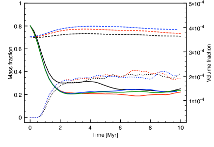
Figure 10.— Same as Fig. 8, but for Run 3 (black), Run 4 (red) and Run 5 (blue). We also plot the volume fraction for Run 6 (green). The mass fraction for Run 6 is plotted in Fig. 15.

For the runs with the Sanchez-Salcedo et al. and Cloudy cooling functions, the gas in the interior of the clouds cools and loses pressure. This, potentially, has a large effect on the cloud evolution. However, by comparing the volume fraction of “GMC” gas in Run 4 and 5 (when the cloud loses internal thermal pressure) with the one in Run 3 (where the internal thermal pressure of the cloud stays constant), we find that the resulting effect is minimal (see Fig. 10). The mass distributions above 10² cm^-3 are nearly identical with a small increase to 75% for Run 4 and to 79% for Run 5 (see Figs. 10 and 9). Also, the amount of gas that ends up in dense clumps is independent of the cooling function. Furthermore, the clouds found in Run 3, 4 and 5 after 10 Myr using the cloud-finding algorithm have similar masses, velocity dispersions and sizes.

Since the gas in the clouds is cold and predominantly molecular, not atomic, we also ran a simulation with the Cloudy cooling function and where we use $\mu=2.33$ instead of $\mu=1.27$. This change does not affect the dynamics of the clouds as can be seen in Figs. 10, 13 and 15.

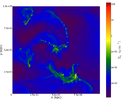
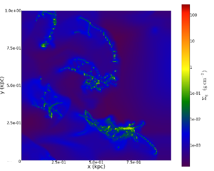
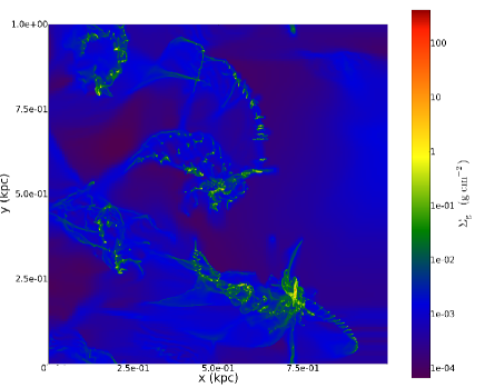
Figure 11.— Same as Fig. 6 but for Run 3 (top left), Run 4 (top right) and Run 5 (bottom).

While the global properties of the clouds are similar, the cloud substructure, i.e. the clump distribution, changes with the cooling function (see Fig. 11). Much more filamentary and clumpy structures are present for the Cloudy cooling function than for the other two. However, this is partly a numerical effect due to the applied refinement criterion and to the timestep used for evolving the simulation. As the different cooling functions tend to cool the gas to different equilibrium temperatures (see Fig. 2), the densities at which a grid cell is refined differ as the gas temperature influences the Jeans length. Such changes introduce small variations in AMR simulations (Niklaus et al., 2009).

3.5. Star Formation

The high resolution simulations described above (Runs 2 - 6) evolve to a state where a large fraction,  40-50%, of the gas is in clumps, as defined by $n_{\rm H}>10^{5}~{}{\rm cm^{-3}}$. Now, in Run 7, we introduce star formation in these objects, following the method described in §2.2. As the density threshold for gas in dense clumps is the same as the critical density of our star formation routine, star particles will form in the dense clumps.

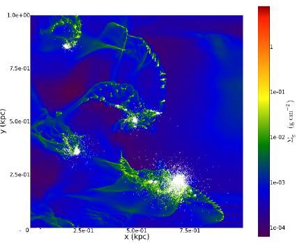
Figure 12.— Same as Fig. 6 but for Run 7. The white dots represent the star particles.

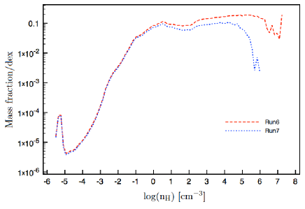
Figure 13.— Mass-weighted PDF for Run 6 (red, dashed) and Run 7 (blue, dotted). We included the stellar mass in the total mass to normalize the distribution function.

Figure 12 shows the gas surface density of Run 7 with the star cluster particles plotted on top. The star cluster particles are concentrated within the molecular clouds. Note, however, that star particles can be ejected from the clouds, especially in clouds with large amounts of angular momentum, e.g. from a collision. The star formation has not changed much of the global density structure or dynamics, but has reduced the maximum gas surface densities by about an order of magnitude compared to Run 6 without star formation. This can also be seen in the PDFs where the star formation process only produces a deviation above $n_{\rm H}\approx 10^{4}$ cm^-3 and limits the maximum density in the simulation to $\approx 10^{6}$ cm^-3 (Fig. 13). As we do not yet include stellar feedback in our simulations, the stars only interact gravitationally with their maternal cloud.

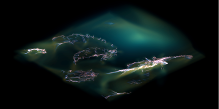
Figure 14.— Volume rendered number density of Run 7. The “GMC” threshold volume density, $n_{\rm H}\sim 100\>{\rm cm^{-3}}$, is coloured blue, while the “Clump” threshold volume density, $n_{\rm H}\sim 10^{5}\>{\rm cm^{-3}}$, gas is coloured red.

Figure 15.— Same as Fig. 8, but for Run 6 (red) and Run 7 (blue). The stellar mass fraction for Run 7 (solid) is also shown. For Run 7 the normalization is done with the sum of the total gas and stellar mass.

Figure 14 shows a rendered visualization of the ISM structures at the end of Run 7, highlighting the volume density thresholds that define “GMCs” and “Clumps”. Several hundred parsec long filaments of high density gas are visible, which bear a qualitative resemblance to some observed Galactic infrared dark cloud structures (e.g. the “Nessie” nebula, Jackson et al., 2010). A comparison of dynamical state of the simulation filaments with observed IRDCs (e.g. Hernandez et al., 2012), will be carried out in a subsequent paper.

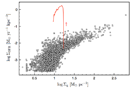
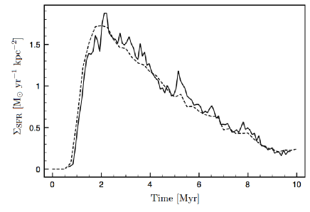
Figure 16.— Left: The star formation rate ($\Sigma_{\rm SFR}$) as function of the gas surface density. The symbols show the observations of Bigiel et al. (2008), while the solid line shows the evolution of $\Sigma_{\rm SFR}$ in Run 7. The arrow shows the direction of the evolution. The star formation rate quickly rises to more than 100 times the observed value — a result both of the initial condition having a relatively high mass fractions of dense gas and the lack of support from magnetic fields or disruption by stellar feedback. Gas is consumed, but the SFR remains about 100 times larger than the levels seen in galactic disks with similar gas content. Right: $\Sigma_{\rm SFR}$ (solid) as function of time for Run 7. The dashed line shows the rescaled mass fraction of gas in dense clumps for Run 7.

The removal of mass from the gas phase because of star formation can be seen by following the gas mass fraction in molecular clouds and in dense clumps for Run 6 and 7 (Fig. 15). After 2 Myr, dense clumps start to form and immediately produce stars. As molecular gas is converted into stars, the mass fraction of gas in molecular clouds starts to decrease (Note that we calculate the mass fraction to the total mass including the stellar mass). After 10 Myr, the mass fraction in “GMCs” in Run 10 is about 60% lower than in Run 6. Similarly, the dense clump mass fraction drops to 2% of the total mass compared to 32% in Run 6. As the stellar mass is about half of the total mass after 10 Myr and star cluster particles only originate within dense clumps, this suggests that the dense clump gas is continuously replenished from the lower density molecular gas. This replenishment, however, does not keep up with the rate at which the dense clumps convert gas into stars. The free-fall time of gas within the clump is shorter than the free-fall time of the region surrounding the clump, i.e. the mean density decreases when including the gas around the clump. Hence, the mass fraction in dense clumps decreases with time. As the star formation rate depends on the gas mass in dense clumps (Eq. 2), the evolution of the star formation rate should follow the curve of the mass fraction of the dense clumps. Figure 16 indeed shows that this is the case with a maximum star formation rate of 1.8 M_☉ yr^-1 kpc^-2 after 2 Myr and then a steady decrease to 0.2 M_☉ yr^-1 kpc^-2 at 10 Myr. This is more than 2 orders of magnitude more than the star formation rates observed by Bigiel et al. (2008) (see Fig. 16).

Of course, the star formation rates in Run 7 depend on the values of the parameters $\epsilon_{\rm ff}$ and potentially on M_∗,min and $n_{\rm H,sf}$ in the star formation routine. We did additional simulations where we varied these parameters. Increasing M_∗,min to 200 M_☉ shortens the run time of the simulation as the number of star particles in the simulation decreases, but it does not change the star formation rate. The total stellar mass only deviated by less than 2%. By changing $n_{\rm H,sf}$ to 10⁴ cm^-3, stars start to form earlier as these densities are reached at earlier times. However, the overall star formation rate is not affected very much: the total stellar mass only increases by 6%. On the other hand, if we increase $n_{\rm H,sf}$ to 10⁶ cm^-3 the stellar mass decreases by $\approx$ 26%. The increased critical density reduces the gas reservoir from which the star particles form, although only by a relatively small amount.

4. Conclusion and discussion

We have investigated the star formation process down to $\lesssim$parsec scales in a galactic disk. We extracted a kiloparsec-scale patch of the disk from the large, global simulation of TT09 and increased the resolution down to 0.5 pc. This allowed us to study the structure and evolution of GMCs in greater detail. We also included additional physics such as heating, atomic and molecular cooling, and a simplified approach to star formation. So far we have neglected the countering effects of magnetic fields and localized stellar feedback.

We used a novel approach to include molecular cooling in our models. The formation of molecules depends strongly on the amount of attenuation of the radiation field. From a high-resolution simulation including the atomic cooling function of Sanchez-Salcedo et al. (2002) that reproduces the equilibrium phase curve of Wolfire et al. (1995) we find that the column extinction can be expressed as a function of gas density. Such a one-to-one relation eliminates the need for time-consuming column-extinction calculations to assess the attenuation of the radiation field in the numerical simulations. We also use this extinction-density relation to generate a table of cooling and heating rates as function of density and temperature with the code Cloudy. The resulting cooling function resembles the atomic cooling function up to densities of 10² cm^-3, above which molecular species start to dominate the cooling rates. However, we need to keep in mind that the heating and cooling rates are only first order approximations as the extinction law is only a mean relation and as local abundance variations and time-dependent chemistry are not considered. Furthermore the simulations do not take into account the local generation of FUV radiation from young star clusters.

With an increased resolution of $\sim 0.5$ pc our simulations are able to capture a significant range of the internal structure of molecular clouds. While the global properties, such as the mass in the molecular clouds, remain the same, filaments and dense clumps form within the clouds shifting the mass distribution towards higher densities. The mass distribution within the molecular clouds are independent of the applied cooling function even though the three cooling functions describe different aspects of the thermal properties of the ISM. This suggests that the thermal pressure is of minor importance within the gravitationally-bound clouds. Then self-gravity and non-thermal motions determine the cloud structure. The nonthermal motions are driven by bulk cloud motions inherited by the GMCs that were formed and evolved in a shearing galactic disk where cloud-cloud collisions are frequent and influence GMC dynamics (TT09, Tan et al. (2012)). Our simulations begin to resolve the cascade of the kinetic energy from these larger scales and processes down to the smaller scales of clumps in the GMCs. This approach is to be contrasted with the method of driving turbulence artificially in periodic box simulations of GMCs (e.g. Schmidt et al., 2010) or of forming GMCs in large-scale converging flows of atomic gas where the turbulence is driven by thermal and dynamical instabilities (e.g. Heitsch et al., 2008; Vázquez-Semadeni et al., 2011).

Of the gas within molecular clouds 50-60% is in dense clumps with $n_{\rm H}>10^{5}\>{\rm cm^{-3}}$. This value is much higher than observed in nearby GMCs, e.g. 90% of the clouds in the Bolocam Galactic Plane Survey have a ratio of clump mass to cloud mass, or clump formation efficiency, between 0 and 0.15 (Eden et al., 2012). The high clump formation efficiency is partly due to our resolution limit. We do not properly capture the formation of individual PSCs. so that the turbulent dissipation range is not fully resolved. The clumps then lack turbulent support against self-gravity hereby attaining higher densities and accumulating more mass.

The surface densities of the clumps in Run 7 are in the range of $\sim$0.1 to $\sim$10 g cm^-2. Galactic IRDCs (e.g. Butler & Tan, 2009, 2012) and star-forming clumps (e.g. Mueller et al., 2002) are found in the range $\sim$0.1 to a few g cm^-2. The most extreme mass surface density clumps seen in our simulations are probably prevented from forming in reality by localized feedback processes from star formation, especially the momentum input from protostellar outflows (Nakamura & Li, 2007).

The star formation rate in our simulations exceeds that expected from the Kennicutt-Schmidt relation (e.g. Bigiel et al., 2011). These authors find a close relation between the surface density of H₂ and the star formation rate surface density for 1 kpc resolution regions within 31 disk galaxies. With a surface density of roughly 8 M_☉ pc^-2 in our simulations, the star formation rate of 0.3 M_☉ yr^-1 kpc^-2 after 10 Myr is about 100 times higher than observed. This over efficiency of star formation in our simulations is a simple reflection of the high mass fraction in dense clumps: while the GMCs are globally stable, there is no support against free-fall collapse in local regions of the GMCs. We can identify two physical mechanisms of reducing this mass fraction: magnetic fields and stellar feedback. From Chandrasekhar & Fermi (1953) we can estimate the critical magnetic field required for support against self-gravity (neglecting the contribution of thermal and turbulent support), i.e.

$$\bar{B}_{\rm crit}=2\pi R\bar{\rho}\sqrt{G}.$$ (9)

Assuming that the clumps in a GMC condense out of local volumes of radius $\sim$ 10 pc and a GMC density of $n_{\rm H}=100~{}{\rm cm^{-3}}$, we find that a mean magnetic field of $\sim$ 10 $\mu$G is sufficient. This is similar to the observationally inferred value at this density (Crutcher et al., 2010). We will study the effect of magnetic support in a subsequent paper.

References

- Audit & Hennebelle (2010) Audit, E., & Hennebelle, P. 2010, A&A, 511, A76
- Bakes & Tielens (1994) Bakes, E. L. O., & Tielens, A. G. G. M. 1994, ApJ, 427, 822
- Baldwin et al. (1991) Baldwin, J. A., Ferland, G. J., Martin, P. G., et al. 1991, ApJ, 374, 580
- Ballesteros-Paredes et al. (2007) Ballesteros-Paredes, J., Klessen, R. S., Mac Low, M.-M., & Vazquez-Semadeni, E. 2007, Protostars and Planets V, 63
- Banerjee et al. (2009) Banerjee, R., Vázquez-Semadeni, E., Hennebelle, P., & Klessen, R. S. 2009, MNRAS, 398, 1082
- Barnes et al. (2011) Barnes, P. J., Yonekura, Y., Fukui, Y., et al. 2011, ApJS, 196, 12
- Bigiel et al. (2008) Bigiel, F., Leroy, A., Walter, F., et al. 2008, AJ, 136, 2846
- Bigiel et al. (2011) Bigiel, F., Leroy, A. K., Walter, F., et al. 2011, ApJ, 730, L13
- Binney & Tremaine (1987) Binney, J., & Tremaine, S. 1987, Princeton, NJ, Princeton University Press, 1987, 747 p.
- Black (1987) Black, J. H. 1987, Interstellar Processes, 134, 731
- Bryan & Norman (1997) Bryan, G. L. & Norman, M. L. 1997, ASP Conf. Ser. 123: Computational Astrophysics; 12th Kingston Meeting on Theoretical Astrophysics, 363
- Bryan (1999) Bryan, G. L. Comp. Phys. and Eng. 1999, 1, 46
- Butler & Tan (2009) Butler, M. J., & Tan, J. C. 2009, ApJ, 696, 484
- Butler & Tan (2012) Butler, M. J., & Tan, J. C. 2012, ApJ, submitted
- Chandrasekhar & Fermi (1953) Chandrasekhar, S., & Fermi, E. 1953, ApJ, 118, 116
- Clark et al. (2012) Clark, P. C., Glover, S. C. O., Klessen, R. S., & Bonnell, I. A. 2012, arXiv:1204.5570
- Crutcher et al. (2010) Crutcher, R. M., Wandelt, B., Heiles, C., Falgarone, E., & Troland, T. H. 2010, ApJ, 725, 466
- Dib et al. (2007) Dib, S., Kim, J., Vazquez-Semadeni, E., Burkert, A., & Shadmehri, M. 2007, ApJ, 661, 262
- Dobbs et al. (2011) Dobbs, C. L., Burkert, A., & Pringle, J. E. 2011, MNRAS, 413, 2935
- Eden et al. (2012) Eden, D. J., Moore, T. J. T., Plume, R., & Morgan, L. K. 2012, MNRAS, 2784
- Elmegreen (2000) Elmegreen, B. G. 2000, ApJ, 530, 277
- Elmegreen (2007) Elmegreen, B. G. 2007, ApJ, 668, 1064
- Elmegreen & Scalo (2004) Elmegreen, B. G., & Scalo, J. 2004, ARA&A, 42, 211
- Federrath et al. (2011) Federrath, C., Sur, S., Schleicher, D. R. G., Banerjee, R., & Klessen, R. S. 2011, ApJ, 731, 62
- Ferland et al. (1998) Ferland, G. J. Korista, K.T. Verner, D.A. Ferguson, J.W. Kingdon, J.B. Verner, & E.M. 1998, PASP, 110, 761
- Field (1965) Field, G. B. 1965, ApJ, 142, 531
- Folini & Walder (1998) Folini, D., & Walder, R. 1998, Astronomische Gesellschaft Meeting Abstracts, 14, 8
- Glover & Clark (2012) Glover, S. C. O., & Clark, P. C. 2012, MNRAS, 421, 9
- Glover & Mac-Low (2007) Glover, S. C. O., & Mac-Low, M.-M., 2007, ApJS, 169, 239
- Glover & Mac-Low (2011) Glover, S. C. O., & Mac Low, M.-M. 2011, MNRAS, 412, 337
- Habing (1968) Habing, H. J. 1968, Bull. Astron. Inst. Netherlands, 19, 421
- Heitsch et al. (2008) Heitsch, F., Hartmann, L. W., Slyz, A. D., Devriendt, J. E. G., & Burkert, A. 2008, ApJ, 674, 316
- Hennebelle et al. (2008) Hennebelle, P., Banerjee, R., Vázquez-Semadeni, E., Klessen, R. S., & Audit, E. 2008, A&A, 486, L43
- Hernandez et al. (2012) Hernandez, A. K., Tan, J. C., Kainulainen, J., Caselli, P., Butler, M. J., Jímenez-Serra, I., & Fontani, F., 2012, ApJ, 756, L13
- Imara et al. (2011) Imara, N., Bigiel, F., & Blitz, L. 2011, ApJ, 732, 79
- Imara & Blitz (2011) Imara, N., & Blitz, L. 2011, ApJ, 732, 78
- Jackson et al. (2010) Jackson, J. M., Finn, S. C., Chambers, E. T., Rathborne, J. M., & Simon, R. 2010, ApJ, 719, L185
- Kawamura et al. (2009) Kawamura, A., Mizuno, Y., Minamidani, T., et al. 2009, ApJS, 184, 1
- Koda et al. (2006) Koda, J., Sawada, T., Hasegawa, T., & Scoville, N. Z. 2006, ApJ, 638, 191
- Koda et al. (2009) Koda, J., Scoville, N., Sawada, T., et al. 2009, ApJ, 700, L132
- Koyama & Inutsuka (2002) Koyama, H., & Inutsuka, S.-I. 2002, ApJ, 564, L97
- Krumholz & McKee (2005) Krumholz, M. R., & McKee, C. F., 2005, ApJ, 630, 250
- Krumholz & Tan (2007) Krumholz, M. R., & Tan, J. C., 2007, ApJ, 654, 304
- Mac Low & Klessen (2004) Mac Low, M.-M., & Klessen, R. S. 2004, Reviews of Modern Physics, 76, 125
- McKee & Ostriker (2007) McKee, C. F., & Ostriker, J. C., 2007, ARA&A, 45, 565
- McKee & Tan (2003) McKee, C. F., & Tan, J. C. 2003, ApJ, 585, 850
- Mueller et al. (2002) Mueller, K. E., Shirley, Y. L., Evans, N. J., II, & Jacobson, H. R. 2002, ApJS , 143, 469
- Nakamura & Li (2007) Nakamura, F., & Li, Z-Y. 2007, ApJ, 662, 395
- Niklaus et al. (2009) Niklaus, M., Schmidt, W., & Niemeyer, J. C. 2009, A&A, 506, 1065
- O’Shea et al. (2004) O’Shea, B. W., Bryan, G., Bordner, J., Norman, M. L., Abel, T., Harkness, R., & Kritsuk, A. 2004, ArXiv Astrophysics e-prints, astro-ph/0403044
- Padoan & Nordlund (2011) Padoan, P., & Nordlund, A., 2011, ApJ, 730, 40
- Roman-Duval et al. (2010) Roman-Duval, J., Jackson, J. M., Heyer, M., Rathborne, J. & Simon, R. 2010, ApJ, 723, 492
- Rosen & Bregman (1995) Rosen, A. & Bregman, J. N. 1995, ApJ, 440, 634
- Rosolowsky et al. (2003) Rosolowsky, E., Engargiola, G., Plambeck, R., & Blitz, L. 2003, ApJ, 599, 258
- Sanchez-Salcedo et al. (2002) Sanchéz-Salcedo, F. J., Vázquez-Semadeni, E. & Gazol, A. 2002, ApJ, 577, 768
- Sarazin & White (1987) Sarazin, C. L. & White, R. E. 1987, ApJ, 320, 32
- Scalo & Elmegreen (2004) Scalo, J., & Elmegreen, B. G. 2004, ARA&A, 42, 275
- Schmidt et al. (2010) Schmidt, W., Kern, S. A. W., Federrath, C., & Klessen, R. S. 2010, A&A, 516, A25
- Shetty et al. (2011a) Shetty, R., Glover, S. C., Dullemond, C. P., & Klessen, R. S. 2011, MNRAS, 412, 1686
- Shetty et al. (2011b) Shetty, R., Glover, S. C., Dullemond, C. P., et al. 2011, MNRAS, 415, 3253
- Smith et al. (2008) Smith, B., Sigurdsson, S., & Abel, T. 2008, MNRAS, 385, 1443
- Smith et al. (2009) Smith, B. D., Turk, M. J., Sigurdsson, S., O’Shea, B. W., & Norman, M. L. 2009, ApJ, 691, 441
- Solomon et al. (1987) Solomon, P. M., Rivolo, A. R., Barrett, J., & Yahil, A. 1987, ApJ, 319, 730
- Tan, Krumholz & McKee (2006) Tan, J. C., Krumholz, M.R., & McKee, C. F. 2006, ApJ, 641, 121
- Tan et al. (2012) Tan, J. C., Shaske, S. N., & Van Loo, S. 2012, arXiv:1211.0198
- Tasker (2011) Tasker, E. J. 2011, ApJ, 700, 358
- Tasker & Tan (2009) Tasker, E. J., & Tan, J. C. 2009, ApJ, 700, 358
- Tielens & Hollenbach (1985) Tielens, A. G. G. M., & Hollenbach, D. 1985, ApJ, 291, 722
- Truelove et al. (1997) Truelove, J. K., Klein, R. I., McKee, C. F., Holliman, J. H., Howell, L. H., & Greenough, J. A. 1997, ApJ, 489, L179
- Turk et al. (2011) Turk, M. J., Smith, B. D., Oishi, J. S., et al. 2011, ApJS, 192, 9
- van Hoof et al. (2004) van Hoof, P. A. M., Weingartner, J. C., Martin, P. G., Volk, K, & Ferland, G. J. 2004, MNRAS, 350, 1330
- van Loo et al. (2007) van Loo, S., Falle, S. A. E. G., Hartquist, T. W., & Moore, T. J. T. 2007, A&A, 471, 213
- van Loo et al. (2010) van Loo, S., Falle, S. A. E. G., & Hartquist, T. W. 2010, MNRAS, 406, 1260
- Vázquez-Semadeni et al. (2003) Vázquez-Semadeni, E., Ballesteros-Paredes, J., & Klessen, R. S. 2003, ApJ, 585, L131
- Vázquez-Semadeni et al. (2011) Vázquez-Semadeni, E., Banerjee, R., Gómez, G. C., et al. 2011, MNRAS, 414, 2511
- Walder & Folini (2000) Walder, R., & Folini, D. 2000, Ap&SS, 274, 343
- Weingartner et al. (2006) Weingartner, J. C., Draine, B. T., & Barr, D. K. 2006, ApJ, 645, 1188
- Wolfire et al. (1995) Wolfire, M. G., Hollenbach, D., McKee, C. F., et al. 1995, ApJ, 443, 152
- Wolfire et al. (2003) Wolfire, M. G., McKee, C. F., Hollenbach, D., & Tielens, A. G. G. M. 2003, ApJ, 587, 278
- Zuckerman & Evans (1974) Zuckerman, B., & Evans, N. J. II, 1974, ApJ, 192, L149