S2LET: A code to perform fast wavelet analysis on the sphere

We describe S2LET, a fast and robust implementation of the scale-discretised wavelet transform on the sphere. Wavelets are constructed through a tiling of the harmonic line and can be used to probe spatially localised, scale-dependent features of signals on the sphere. The reconstruction of a signal from its wavelets coefficients is made exact here through the use of a sampling theorem on the sphere. Moreover, a multiresolution algorithm is presented to capture all information of each wavelet scale in the minimal number of samples on the sphere. In addition S2LET supports the HEALPix pixelisation scheme, in which case the transform is not exact but nevertheless achieves good numerical accuracy. The core routines of S2LET are written in C and have interfaces in Matlab, IDL and Java. Real signals can be written to and read from FITS files and plotted as Mollweide projections. The S2LET code is made publicly available, is extensively documented, and ships with several examples in the four languages supported. At present the code is restricted to axisymmetric wavelets but will be extended to directional, steerable wavelets in a future release.

1 Introduction

Signals defined or measured on the sphere arise in numerous disciplines, where analysis techniques defined explicitly on the sphere are now in common use. In particular, wavelets on the sphere (Antoine & Vandergheynst 1998, 1999; Baldi et al. 2009; Marinucci et al. 2008; McEwen et al. 2006; Narcowich et al. 2006; Starck et al. 2006a; Wiaux et al. 2006, 2005, 2007, 2008; Yeo et al. 2008) have been applied very successfully to problems in astrophysics and cosmology, where data-sets are increasingly large and need to be analysed at high resolution in order to confront accurate theoretical predictions (e.g. Barreiro et al. 2000; Basak & Delabrouille 2012; Cayón et al. 2001; Deriaz et al. 2012; Labatie et al. 2012; Lan & Marinucci 2008; McEwen et al. 2006, 2007a, 2007b, 2008; Pietrobon et al. 2008; Starck et al. 2006b; Schmitt et al. 2010; Vielva et al. 2004, 2006a, 2006b, 2007; Wiaux et al. 2006, 2008).

While wavelet theory is well established in Euclidean space (see e.g. Daubechies 1992), multiple wavelet frameworks have been developed on the sphere, only a fraction of which lead to exact transforms in both the continuous and discrete settings. In fact, discrete methodologies (Schröder & Sweldens 1995; Sweldens 1996, 1997) achieve exactness in practice but may not lead to a stable basis on the sphere (Sweldens 1997). In the continuous setting several constructions are theoretically exact, and have been combined with sampling theorems on the sphere to enable exact reconstruction in the discrete setting also. In particular, scale-discretised wavelets (Wiaux et al. 2008) lean on a tiling of the harmonic line to yield an exact wavelet transform in both the continuous and discrete settings. In the axisymmetric case, the scale-discretised wavelets reduce to needlets (Narcowich et al. 2006; Baldi et al. 2009; Marinucci et al. 2008), which were developed independently using an analogous tiling of the harmonic line. Similarly, the isotropic undecimated wavelet transform (UWT) developed by (Starck et al. 2006a) exploits B-splines of order 3 to cover the harmonic line with filters with greater overlap but nevertheless compact support.

In this paper we describe the new publicly available S2LET code to perform the scale-discretised wavelet transform of complex signals on the sphere. At present S2LET is restricted to axisymmetric wavelets (i.e. azimuthally symmetric when centred on the poles) and includes generating functions for axisymmetric scale-discretised wavelets (Wiaux et al. 2008), needlets (Narcowich et al. 2006; Baldi et al. 2009; Marinucci et al. 2008) and B-spline wavelets (Starck et al. 2006a). We intend to extend the code to directional, steerable wavelets and spin functions in a future release. The core routines of S2LET are written in C, exploit fast algorithms on the sphere, and have interfaces in Matlab, IDL and Java.

We note that many very useful public codes are already available to compute wavelet transforms on the sphere, including isotropic undecimated wavelet, ridgelet and curvelet transforms (Starck et al. 2006a), invertible filter banks (Yeo et al. 2008), needlets (NeedATool; Pietrobon et al. 2010) and scale-discretised wavelets (S2DW; Wiaux et al. 2008). S2LET aims primarily to provide a fast and flexible implementation of the scale-discretised transform with exact reconstruction on the sphere using the sampling theorem of McEwen & Wiaux (2011), although it has also been extended to support some of the features of these other codes. Furthermore, particular attention has been paid in the development of S2LET to prove a user-friendly code, supporting multiple programming languages, and which is extensively documented.

The remainder of this article is organised as follows. In section 2 we detail the construction of scale-discretised axisymmetric wavelets and the corresponding exact scale-discretised wavelet transform on the sphere. In section 3 we describe the S2LET code, including implementation details, computational complexity and numerical performance. We present a number of simple examples using S2LET in section 4, along with the code to execute them. We conclude in section 5.

2 Wavelets on the sphere

We review the construction of scale-discretised wavelets on the sphere through tiling of the harmonic line (Wiaux et al. 2008). Directional, steerable wavelets were also considered by Wiaux et al. (2008), however we restrict our attention to axisymmetric wavelets here. Furthermore, the use of a sampling theorem on the sphere guarantees that spherical harmonic coefficients capture all the information content of band-limited signals, resulting in theoretically exact harmonic and wavelet transforms. One may alternatively adopt samplings of the sphere for which exact quadrature rules do not exist, such as HEALPix (Górski et al. 2005), but which nevertheless exhibit other useful properties, leading to numerically accurate but not theoretically exact transforms.

2.1 Harmonic analysis on the sphere

The spherical harmonic decomposition of a square integrable signal $f\in L^{2}(S^{2})$ on the two-dimensional sphere $S^{2}$ reads

$$f(\omega)=\sum_{\ell=0}^{\infty}\sum_{m=-\ell}^{\ell}f_{\ell m}Y_{\ell m}(\omega),$$ (1)

where $Y_{\ell m}$ are the spherical harmonic functions, which form the canonical orthogonal basis on $S^{2}$. The spherical harmonic coefficients $f_{\ell m}$, with $\ell\in\mathbb{N}$ and $m\in\mathbb{Z}$ such that $|m|\leq\ell$, form a dual representation of the signal $f$ in the harmonic basis on the sphere. The angular position $\omega=(\theta,\phi)\in S^{2}$ is specified by colatitude $\theta\in[0,\pi]$ and longitude $\phi\in[0,2\pi)$. The spherical harmonic coefficients are given by

$$f_{\ell m}=\langle f|Y_{\ell m}\rangle=\int_{S^{2}}{\rm d}\Omega(\omega)f(\omega)Y^{*}_{\ell m}(\omega),$$ (2)

with the surface element ${\rm d}\Omega(\omega)=\sin\theta{\rm d}\theta{\rm d}\phi$. We consider band-limited signals in the spherical harmonic basis, with band-limit $L$ if $f_{\ell m}=0,\ \forall\ell\geq L$. For band-limited signals sampling theorems can be invoked so that both forward and inverse transforms can be reduced to finite summations that are theoretically exact. Sampling theorems effectively encode a quadrature rule for the exact evaluation of integrals on the sphere from a finite set of sampling nodes. Various sampling theorems exist in the literature (e.g. Driscoll & Healy 1994; Healy et al. 1996; McEwen & Wiaux 2011). In this work we adopt the McEwen & Wiaux (2011) sampling theorem (hereafter MW), which is based on an equiangular sampling scheme and, for a given band-limit $L$, requires the lowest number of samples on the sphere of all sampling theorems, namely $(L-1)(2L-1)+1\sim 2L^{2}$ samples (for comparison $\sim 4L^{2}$ samples are required by Driscoll & Healy (1994)). Fast algorithms to compute the corresponding spherical harmonic transform scale as $\mathcal{O}(L^{3})$ and are numerically stable to band-limits of at least $L=4096$ (McEwen & Wiaux 2011). The GLESP pixelisation scheme (Doroshkevich et al. 2005) also provides a sampling theorem based on the Gauss-Legendre quadrature, and could be used in place of the MW sampling theorem. However, GLESP uses more samples than Gauss-Legendre quadrature requires, which may lead to an overhead when considering large band-limits and numerous wavelet scales. We focus on the MW sampling scheme to obtain a theoretically exact transform. Alternative sampling schemes that are not based on sampling theorems also exist such as HEALPix (Górski et al. 2005), which is supported by S2LET, MRS and Needatool. HEALPix does not lead to exact transforms on the sphere but the resulting approximate transforms nevertheless achieve good accuracy and benefit from other practical advantages, such as equal-area pixels.

2.2 Scale-discretised wavelets on the sphere

The scale-discretised wavelet transform allows one to probe spatially localised, scale-dependent content in the signal of interest $f\in L^{2}(S^{2})$. The $j$-th wavelet scale $W^{\Psi^{j}}\in L^{2}(S^{2})$ is defined as the convolution of $f$ with the wavelet $\Psi^{j}\in L^{2}(S^{2})$:

$$W^{\Psi^{j}}(\omega) \equiv(f\star\Psi^{j})(\omega)\equiv\langle f|\mathcal{R}_{\omega}\Psi^{j}\rangle$$

$$\equiv\int_{S^{2}}{\rm d}\Omega(\omega^{\prime})f(\omega^{\prime})(\mathcal{R}_{\omega}\Psi^{j})^{*}(\omega^{\prime}),$$ (3)

where ^∗ denotes complex conjugation. Convolution on the sphere is defined by the inner product of $f$ with the rotated wavelet $\mathcal{R}_{\omega}\Psi^{j}$. We restrict our attention to axisymmetric wavelets, i.e. wavelets that are azimuthally symmetric when centred on the poles. Consequently, the rotation operator $\mathcal{R}_{\omega}$ is parameterised by angular position $\omega=(\theta,\phi)$ only and not also orientation. For the axisymmetric case the spherical harmonic decomposition of $W^{\Psi^{j}}$ is then simply given by a weighted product in harmonic space:

$${W}^{\Psi^{j}}_{\ell m}=\sqrt{\frac{4\pi}{2\ell+1}}{f}_{\ell m}{\Psi}^{j*}_{\ell 0},$$ (4)

where ${W}^{\Psi^{j}}_{\ell m}=\langle W^{\Psi^{j}}|Y_{\ell m}\rangle$, $f_{\ell m}=\langle f|Y_{\ell m}\rangle$ and ${\Psi}^{j}_{\ell 0}\delta_{m0}=\langle\Psi^{j}|Y_{\ell m}\rangle$, and where $\delta_{m0}$ is the Kronecker delta symbol.

The wavelet coefficients extract the detail information of the signal only; a scaling function and corresponding scaling coefficients must be introduced to represent the low-frequency (low-$\ell$), approximate information of the signal. The scaling coefficients $W^{\Phi}\in L^{2}(S^{2})$ are defined by the convolution of $f$ with the scaling function $\Phi\in L^{2}(S^{2})$:

$$W^{\Phi}(\omega)\equiv(f\star\Phi)(\omega)=\langle f|\mathcal{R}_{\omega}\Phi\rangle,$$ (5)

or in harmonic space,

$${W}^{\Phi}_{\ell m}=\sqrt{\frac{4\pi}{2\ell+1}}{f}_{\ell m}{\Phi}^{*}_{\ell 0},$$ (6)

where ${W}^{\Phi}_{\ell m}=\langle W^{\Phi}|Y_{\ell m}\rangle$ and ${\Phi}_{\ell 0}\delta_{m0}=\langle\Phi|Y_{\ell m}\rangle$.

Provided the wavelets and scaling function satisfy an admissibility property (defined below), the function $f$ may be reconstructed exactly from its wavelet and scaling coefficients by

$$\quad f(\omega)= \int_{S^{2}}{\rm d}\Omega(\omega^{\prime})W^{\Phi}(\omega^{\prime})(\mathcal{R}_{\omega^{\prime}}\Phi)(\omega)$$

$$+\ \sum_{j=J_{0}}^{J}\int_{S^{2}}{\rm d}\Omega(\omega^{\prime})W^{\Psi^{j}}(\omega^{\prime})(\mathcal{R}_{\omega^{\prime}}\Psi^{j})(\omega),$$ (7)

or equivalently in harmonic space by

$${f}_{\ell m}=\sqrt{\frac{4\pi}{2\ell+1}}{W}^{\Phi}_{\ell m}{\Phi}_{\ell 0}\ +\ \sqrt{\frac{4\pi}{2\ell+1}}\sum_{j=J_{0}}^{J}{W}^{\Psi^{j}}_{\ell m}{\Psi}^{j}_{\ell 0}.$$ (8)

The parameters $J_{0}$, $J$ define the lowest and highest scales $j$ of the wavelet decomposition and must be defined consistently to extract and reconstruct all the information content of $f$. These parameters depend on the construction of the wavelets and scaling function and are defined explicitly in the next paragraphs. The admissibility condition under which a band-limited function $f$ can be decomposed and reconstructed exactly is given by the following resolution of the identity:

$$\frac{4\pi}{2\ell+1}\left(|{\Phi}_{\ell 0}|^{2}+\sum_{j=J_{0}}^{J}|{\Psi}^{j}_{\ell 0}|^{2}\right)\ =\ 1,\quad\forall\ell.$$ (9)

We are now in a position to define wavelets and a scaling function that satisfy the admissibility property. In this paper, we use the smooth generating functions defined by Wiaux et al. (2008) in order to tile the harmonic line. Alternative definitions are also supported by S2LET, as presented at the end of this section. Consider the $C^{\infty}$ Schwartz function with compact support on $[-1,1]$:

$$s(t)\equiv\left\{\begin{array}[]{ll}\ e^{-\frac{1}{1-t^{2}}},&t\in[-1,1]\\ \ 0,&t\notin[-1,1]\end{array}\right.,$$ (10)

for $t\in\mathbb{R}$. We introduce the positive real parameter $\lambda\in\mathbb{R}^{+}_{*}$ to map $s(t)$ to

$$s_{\lambda}(t)\equiv s\left(\frac{2\lambda}{\lambda-1}(t-1/\lambda)-1\right),$$ (11)

which has compact support in $[1/\lambda,1]$. We then define the smoothly decreasing function $k_{\lambda}$ by

$$k_{\lambda}(t)\equiv\frac{\int_{t}^{1}\frac{{\rm d}t^{\prime}}{t^{\prime}}s_{\lambda}^{2}(t^{\prime})}{\int_{1/\lambda}^{1}\frac{{\rm d}t^{\prime}}{t^{\prime}}s_{\lambda}^{2}(t^{\prime})},$$ (12)

which is unity for $t<1/\lambda$, zero for $t>1$, and is smoothly decreasing from unity to zero for $t\in[1/\lambda,1]$. We finally define the wavelet generating function by

$$\kappa_{\lambda}(t)\equiv\sqrt{k_{\lambda}(t/\lambda)-k_{\lambda}(t)}$$ (13)

and the scaling function generating function by

$$\eta_{\lambda}(t)\equiv\sqrt{k_{\lambda}(t)}.$$ (14)

The wavelets and scaling function are constructed from their generating functions to satisfy the admissibility condition given by Eqn. (9). A natural approach is to define ${\Psi}^{j}_{\ell m}$ from the generating functions $\kappa_{\lambda}$ to have support on $[\lambda^{j-1},\lambda^{j+1}]$, yielding

$${\Psi}^{j}_{\ell m}\equiv\sqrt{\frac{2\ell+1}{4\pi}}\ \kappa_{\lambda}\left(\frac{\ell}{\lambda^{j}}\right)\delta_{m0}.$$ (15)

For these wavelets Eqn. (9) is satisfied for $\ell\geq\lambda^{J_{0}}$, where $J_{0}$ is the lowest wavelet scale used in the decomposition. The scaling function $\Phi$ is constructed to extract the modes that cannot be probed by the wavelets (i.e. modes with $\ell<\lambda^{J_{0}}$):

$${\Phi}_{\ell m}\equiv\sqrt{\frac{2\ell+1}{4\pi}}\ \eta_{\lambda}\left(\frac{\ell}{\lambda^{J_{0}}}\right)\delta_{m0}.$$ (16)

To satisfy exact reconstruction, $J$ is set to ensure the wavelets reach the band-limit of the signal of interest, yielding $J=\lceil\log_{\lambda}(L-1)\rceil$. The choice of the lowest wavelet scale $J_{0}$ is arbitrary, provided that $0\leq J_{0}<J$. The wavelets and scaling function may then be reconstructed on the sphere through an inverse spherical harmonic transform. The harmonic tiling and real space representation of these wavelets are shown in Figure 1 and Figure 2 respectively.

In addition to the scale-discretised generating functions (Wiaux et al. 2008), S2LET also supports the needlet functions (Marinucci et al. 2008), which yield a similar tiling of the harmonic line, as shown in Figure 1. The B-spline filters used to construct the isotropic undecimated wavelet transform (Starck et al. 2006a) are also supported, as also shown in Figure 1. With these three constructions, the wavelets and scaling functions are well-localised both spatially on the sphere and also in harmonic space. Consequently, the associated wavelet transforms on the sphere can be used to extract spatially localised, scale-dependent features in signals of interest.

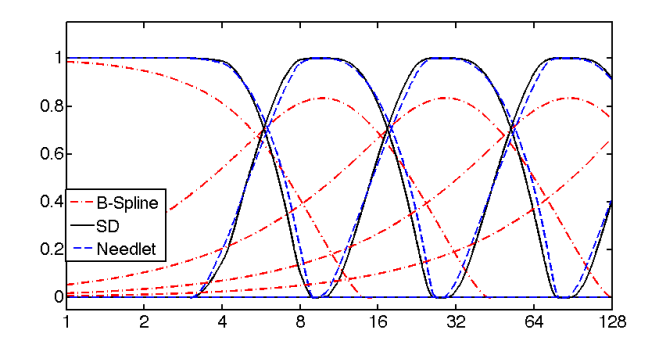
(a) Tiling of the harmonic line

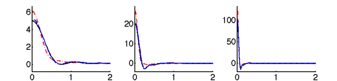
(b) Angular profiles of the scaling function and the first wavelets

Figure 1: Wavelets and scaling function constructed with the scale-discretised (SD), needlet and B-spline generating functions (Wiaux et al. 2008; Marinucci et al. 2008; Starck et al. 2006a) with parameters $\lambda=3$ and $J_{0}=2$ and for band-limit $L=128$. The tiling is shown in the top panel, and the profiles of the reconstructed wavelets in the bottom panel.

Figure 2: Wavelets for scales $j\in\{2,3,4,5\}$ and scaling function constructed through a tiling of the harmonic line using scale-discretised functions, with parameters $\lambda=3$ and $J_{0}=2$ and for band-limit $L=128$. This plot was produced with a Matlab demo included in S2LET.

3 The S2LET code

In this section we describe the S2LET code. We first introduce a multiresolution algorithm to capture each wavelet scale in the minimum number of samples on the sphere, which follows by taking advantage of the reduced band-limit of the wavelets for scales $j<J-1$. This multiresolution algorithm reduces the computation cost of the transform considerably. We then provide details of the implementation, the computational complexity and the numerical accuracy of the scale-discretised wavelet transform supported in S2LET. We finally outline planned future extensions of the code.

3.1 Multiresolution algorithm

In harmonic space, the wavelet coefficients are simply given by the weighted product of the spherical harmonic coefficients of $f$ and the wavelets, as expressed in Eqn. (4). Although the wavelet coefficients can be analysed at the same resolution as the signal $f$ (i.e., at full resolution), by construction they have different band-limits for different scales $j$, as shown in Figure 1. The reconstruction can thus be performed at lower resolution, without any loss of information if a sampling theorem is used. This approach yields a multiresolution algorithm where the wavelet coefficients are reconstructed with the minimal number of samples on the sphere: the $j$-th wavelet coefficients have band-limit $k=\lambda^{j+1}$ when using the scale-discretised and needlet kernels, and $k=L/\lambda^{J-j-2}$ when using the B-splines. When the MW sampling theorem is used, the wavelets are recovered on $(k-1)(2k-1)+1$ samples on the sphere. This approach leads to significant improvements in terms of speed and memory use compared to the full-resolution case, as shown in the next section. Figure 3 illustrates the use of the full-resolution and multiresolution transforms on a map of Earth topography data with the scale-discretised filters and the MW scheme. When adopting the HEALPix sampling of the sphere, multiresolution can also be used. However HEALPix does not rely on a sampling theorem and therefore the resolution for the reconstruction of each wavelet scale must be chosen heuristically and adapted to the desired accuracy. For example, in the MRS code (Starck et al. 2006a) it is chosen such that $N_{\rm side}^{j}=k/2$. More detail on the accuracy of the wavelet transform with HEALPix are provided below.

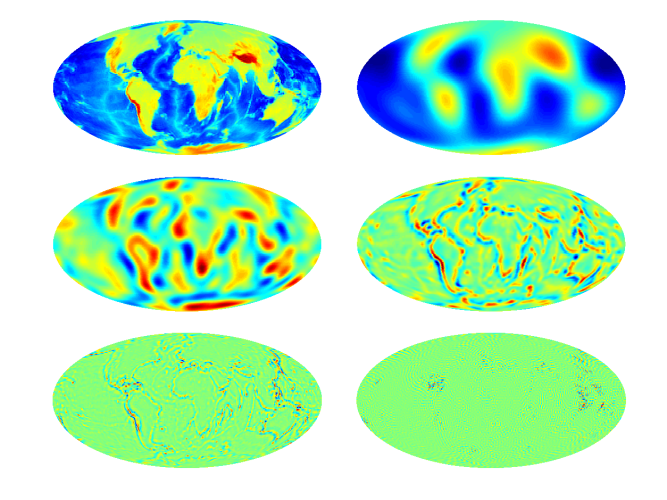
(a) Full-resolution scale-discretised wavelet transform

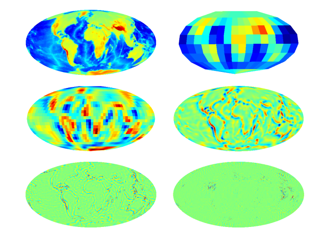
(b) Multiresolution scale-discretised wavelet transform

Figure 3: Scale-discretised wavelet transform of a band-limited topography map of the Earth for $\lambda=3$, $J_{0}=2$ and $L=128$, i.e. with the scale-discretised wavelets shown in Figure 2. The wavelet transform decomposes the band-limited signal into wavelet coefficients that extract spatially localised, scale-dependent features. Since the wavelets for different scales $j$ have different band-limits, the wavelet coefficients can be reconstructed at lower resolution on the sphere for lower scales $j$. Panel (a) shows the full-resolution wavelet transform of the topography map. The original Earth topography map is shown in the top-left plot, the scaling coefficients are shown in the top-right plot, while the wavelet coefficients at scales $j\in\{2,3,4,5\}$ are shown left-to-right, top-to-bottom respectively in the remaining plots. Panel (b) shows the same decomposition but using the multiresolution algorithm. The signals shown in panel (b) contain the same information as in panel (a) but represented in the minimal number of samples on the sphere. These plots were produced by one of the many Matlab demos provided with S2LET.

3.2 Implementation

The core numerical routines of S2LET are implemented in C. By adopting a low level programming language such as C for the implementation of the core algorithms, computational efficiency is optimised. The C library includes the full-resolution and multiresolution wavelet transforms, with specific optimisations for real signals in order to take advantage of all symmetries of the spherical harmonic transform. The wavelet transform is computed in harmonic space through Eqn. (4) and Eqn. (6), for the input parameters $(L,\lambda,J_{0})$. To reconstruct signals on the sphere, by default S2LET uses the exact spherical harmonic transform of the MW sampling theorem (McEwen & Wiaux 2011) implemented in the SSHT code. In this case all transforms are theoretically exact and one can analyse and synthesise real and complex signals at floating-point precision. S2LET has been extended to also support the HEALPix sampling scheme, in which case the transform is not theoretically exact but nevertheless achieves good numerical accuracy.

We provide interfaces for the C library in three languages: Matlab, IDL and Java. The Matlab and IDL codes also include routines to read/write signals on the sphere stored in either HEALPix FITS files or the FITS file format used to stored MW sampled signals. In addition, functionality to plot the Mollweide projection of real signals for both MW or HEALPix samplings is included. The Java interface includes an object-oriented representation of sampled maps, spherical harmonics and wavelet transforms. All routines and interfaces are well documented and illustrated with several examples for both the MW and HEALPix samplings. These examples cover multiple combinations of parameters and types of signals. S2LET requires SSHT, which implements fast and exact algorithms to perform the forward and inverse spherical harmonic transforms corresponding to the MW sampling theorem (McEwen & Wiaux 2011). SSHT in turn requires the FFTW package for the computation of fast Fourier transforms. The fast spherical harmonic transforms implemented in SSHT compute Wigner functions, and thus the spherical harmonic functions, through efficient recursion using either the method of Trapani & Navaza (2006) or Risbo (1996). Here we present results using the recursion of Risbo (1996). The fast spherical harmonic transform algorithms implemented in SSHT scale as $\mathcal{O}(L^{3})$ (McEwen & Wiaux 2011).

Although primarily intended to perform the scale-discretised wavelet transform of Wiaux et al. (2008), S2LET also supports the needlet and spline-based wavelet transforms developed by Marinucci et al. (2008) and Starck et al. (2006a). As shown in Figure 1, these generating functions yield the same number of wavelet scales (for the parameter choices described previously). However, with the scale-discretised and needlet generating functions the $j$-th wavelet scale has compact support in $[\lambda^{j-1},\lambda^{j+1}]$, whereas the support is much wider with the B-splines, i.e. $[0,L/\lambda^{J-j-2}]$ in the S2LET implementation. As a consequence, when using the multiresolution algorithm the wavelet coefficients must be captured on a greater number of pixels than with the scale-discretised or needlet kernels, while probing approximately the same scales, as shown in Figure 1.

The complexity of the axisymmetric wavelet transform is dominated by spherical harmonic transforms since the wavelet transforms are computed efficiently in harmonic space, through Eqn. (4) and Eqn. (6) for the forward transform and through Eqn. (8) for the inverse transform. Given a band-limit $L$ and wavelet parameters $(\lambda,J_{0})$, recall that the maximum scale is given by $J=\lceil\log_{\lambda}(L-1)\rceil$ and hence the wavelet transform (forward or inverse) involves $(J-J_{0}+3)$ spherical harmonic transforms (one for the original signal, one for the scaling coefficients and $(J-J_{0}+1)$ for the wavelet coefficients). If the scaling coefficients and all wavelet coefficients are reconstructed at full-resolution in real space, the axisymmetric wavelet transform scales as $\mathcal{O}((J-J_{0}+3){L^{3}})$. However, in the previous section we established a multiresolution algorithm that takes advantage of the reduced band-limit of the wavelets for scales $j<J-1$. With the multiresolution algorithm with a sampling theorem, only the finest wavelet scales $j\in\{J-1,J\}$ are computed at maximal resolution corresponding to the band-limit of the signal. The complexity of the overall multiresolution wavelet transform is then dominated by these operations and effectively scales as $\mathcal{O}({L^{3}})$.

3.3 Numerical validation

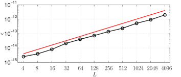
(a) Numerical accuracy of the wavelet transform

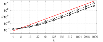
(b) Computation time of the wavelet transform

Figure 4: Numerical accuracy and computation time of the scale-discretised wavelet transform computed with S2LET. We consider $L=2^{i}$ with $i\in\{2,\ldots,10\}$, with parameters $\lambda=2$, $J_{0}=0$. These results are averaged over many realisations of random band-limited signals and were found to be very stable. The scale-discretised transform is either performed at full-resolution (solid lines) or with the multiresolution algorithm (dashed lines). Very good numerical accuracy is achieved by both the full-resolution and multiresolution algorithms (which achieve indistinguishable accuracy), with numerical errors comparable to floating-point precision, found empirically to scale as $\mathcal{O}(L)$ as shown by the red line in panel (a). Computation time scales as $\mathcal{O}(L^{3})$ for both algorithms as shown by the red line in panel (b), in agreement with theory. The multiresolution algorithm is four to five times faster than the full-resolution approach for the band-limits considered.

We first evaluate the performance of S2LET in terms of accuracy and complexity using the MW sampling theorem, for which all transforms are theoretically exact. We show that S2LET achieves floating-point precision and scales as detailed in the previous section.

We consider band-limits $L=2^{i}$ with $i\in\{2,\ldots,10\}$ and generate sets of spherical harmonic coefficients $f_{\ell m}$ following independent Gaussian distributions $\mathcal{N}(0,1)$. We then perform the wavelet decomposition and reconstruct the harmonic coefficients, denoted by $f_{\ell m}^{\textrm{rec}}$. We evaluate the accuracy of the transform using the error metric $\epsilon=\max|f_{\ell m}-f_{\ell m}^{\textrm{rec}}|$, which is theoretically zero since all signals are band-limited by construction. The complexity is quantified by observing how the computation time $t_{\rm c}=[t_{\textrm{synthesis}}+t_{\textrm{analysis}}]/2$ scales with band-limit, where the synthesis and analysis computation times are specified by $t_{\textrm{synthesis}}$ and $t_{\textrm{analysis}}$ respectively. Since we evaluate the wavelet transform in real space, a preliminary step is required to reconstruct the signal $f$ from the randomly generated $f_{\ell m}$. This step is not included in the computation time since its only purpose is to generate a valid band-limited test signal on the sphere. The analysis then denotes the decomposition of $f$ into wavelet coefficients $W^{{\Psi}^{j}}$ and scaling coefficients $W^{\Phi}$ on the sphere. The synthesis refers to recovering the signal $f^{\textrm{rec}}$ from these coefficients. The final step, which is not included in the computation time either, is to decompose $f^{\textrm{rec}}$ into harmonic coefficients $f^{\textrm{rec}}_{\ell m}$ in order to compare them with $f_{\ell m}$. The stability of both $\epsilon$ and $t_{\rm c}$ is checked by averaging over hundreds of realisations of $f_{\ell m}$ for $L=2^{i}$ with $i\in\{2,\ldots,8\}$ and a few realisations with $i\in\{9,10\}$. The results proved to be very stable, i.e. the variances of the error and timing metrics are lower than 5%. Recall that for given band-limit $L$ the number of samples on the sphere required by the exact quadrature is $(2L-1)(L-1)+1$. All tests were run on an Intel 2.0GHz Core i7 processor with 8GB of RAM. On this machine, precision of floating point numbers is of the order of $\sim 10^{-16}$, and errors are expected to add up and accumulate when considering linear operations such as the spherical harmonic and wavelet transforms. The accuracy and timing performance of the scale-discretised wavelet transform implemented in S2LET are presented in Figure 4. S2LET achieves very good numerical accuracy, with numerical errors comparable to accumulated floating-point errors only. Moreover, the full-resolution and multiresolution algorithms are indistinguishable in terms of accuracy. However, the latter is four to five times faster than the former for the band-limits considered since only the wavelet coefficients for $j\in\{J-1,J\}$ are computed at full-resolution. As shown in Figure 4, computation time scales as $\mathcal{O}({L^{3}})$ for both algorithms, in agreement with theory.

S2LET can also be used with HEALPix, in which case the accuracy of the spherical harmonic transform is critical to the accuracy of the wavelet transform (since HEALpix does not rely on a sampling theorem it does not exhibit theoretically exact harmonic transforms, unlike SSHT or GLESP). The performances of the spherical harmonic transforms in HEALPix and GLESP have been widely studied in the past (see, e.g., Reinecke 2011; Doroshkevich et al. 2011; Reinecke & Seljebotn 2013), and that of the MW sampling were presented in McEwen & Wiaux (2011). We do not compile the entirety of these results here, but we have reproduced the essential results on our machine; Table 1 summarises the orders of accuracy of the HEALPix iterative spherical harmonic transform. Using the same setup as previously, we calculated the maximum error on the spherical harmonic coefficients when performing the transform back and forth, averaged over the values of $N_{\rm side}$, since the results were found to be sensitive only to the ratio $L/N_{\rm side}$. Even with several iterations, which multiplies the number of transforms and thus computation time, the spherical harmonic transform in HEALPix remains at least an order of magnitude less accurate than the MW and GLESP counterparts (which, being both theoretically exact, achieve comparable performances, see Reinecke 2011; Reinecke & Seljebotn 2013; Doroshkevich et al. 2011; McEwen & Wiaux 2011). Since the wavelet transforms implemented in MRS and Needatool are also computed in harmonic space, their complexity and accuracy are dominated by that of the underlying spherical harmonic transforms. As a consequence, when adopting the HEALPix scheme, S2LET, MRS and Needatool achieve similar performances, resulting from the computation time and accumulated errors of $(J-J_{0}+1)$ HEALPix spherical harmonic transforms. In the multiresolution case, the results depend on the resolution chosen to reconstruct each wavelet scale.

$\max|f_{\ell m}-f_{\ell m}^{\textrm{rec}}|$	$L=N_{\rm side}/2$	$L=N_{\rm side}$	$L=2N_{\rm side}$	$L=3N_{\rm side}$
0 iteration	$\sim 10^{-6}$	$\sim 10^{-4}$	$\sim 10^{-2}$	$\sim 10^{-1}$
1 iterations	$\sim 10^{-10}$	$\sim 10^{-7}$	$\sim 10^{-3}$	$\sim 10^{-1}$
2 iterations	$\sim 10^{-14}$	$\sim 10^{-10}$	$\sim 10^{-5}$	$\sim 10^{-1}$
3 iterations	$\sim 10^{-14}$	$\sim 10^{-13}$	$\sim 10^{-6}$	$\sim 10^{-1}$
4 iterations	$\sim 10^{-14}$	$\sim 10^{-14}$	$\sim 10^{-7}$	$\sim 10^{-1}$

Table 1: Order of magnitude of the accuracy of the HEALPix spherical harmonic transform, averaged over the parameter $N_{\rm side}$.

3.4 Future extensions

In future work we plan to extend S2LET to support directional, steerable wavelets on the sphere (Wiaux et al. 2008). We also plan to exploit recent ideas leading to fast (spin) spherical harmonic transforms (McEwen & Wiaux 2011) to yield faster algorithms than those developed by Wiaux et al. (2008) and McEwen et al. (2013) to compute directional wavelet transforms on the sphere. Finally, we intend to add support to analyse spin signals on the sphere (c.f. Geller et al. 2008; Geller & Marinucci 2010; Starck et al. 2009). In a future release, the code will also be parallelised, which will lead to further speed improvements. The S2LET code will thus be under active development with future releases forthcoming. In any case, we hope this first version of the S2LET code will prove useful for axisymmetric scale-discretised wavelet analysis on the sphere. Indeed, the code has already been used as an integral part of the new exact flaglet wavelet transform on the ball (Leistedt & McEwen 2012), the spherical space constructed by augmenting the sphere with the radial line.

4 Examples

The S2LET code is extensively documented and ships with several examples in the four languages supported. In this section we present a subset of short examples, along with the code to execute them in order to demonstrate the ease of using S2LET to perform wavelet transforms. All examples were run with the scale-discretised wavelet generating functions.

4.1 Wavelet transform from the command line

S2LET includes ready-to-use high-level programs to directly decompose a real signal into wavelet coefficients. The inputs are a FITS file containing the signal of interest and the parameters for the transform. The program writes the output coefficients in FITS files in the same directory as the input file and with a consistent naming scheme. These commands are available for both HEALPix and MW sampling schemes. For the MW sampling case illustrated in Example 1, the wavelet transform is theoretically exact and the band limit corresponds to the resolution of the input map, which will be read automatically from the file. The transform may be performed in full-resolution or multiresolution by adjusting the multiresolution flag specified by the last parameter (respectively $0$ and $1$), and the output wavelet coefficients are computed at full and minimal resolution accordingly. For the case of a HEALPix map, as illustrated in Example 2, the band-limit must be supplied as the last parameter in the command. The output scaling and wavelet coefficients of a HEALPix map are reconstructed and stored in FITS files at the same resolution as the input map. For both MW and HEALPix samplings the output coefficients may be read and plotted using the Matlab or IDL routines.

⬇

>> ./bin/s2let_axisym_mw_analysis_real <inputFitsFile> <lambda> <J_0> <multiresFlag>

>> ./bin/s2let_axisym_mw_synthesis_real <outputRoot> <lambda> <J_0> <bandLimit>

Example 1: Performing the forward (analysis) and inverse (synthesis) wavelet transform of a real signal (MW sampling) from the command line.

⬇

>> ./bin/s2let_axisym_hpx_analysis_real <inputFitsFile> <lambda> <J_0> <bandLimit>

>> ./bin/s2let_axisym_hpx_synthesis_real <outputRoot> <lambda> <J_0> <bandLimit>

Example 2: Performing the forward (analysis) and inverse (synthesis) wavelet transform of a real signal (HEALPix sampling) from the command line.

4.2 Wavelet transform in Matlab and IDL

Examples 3 and 4 read real signals on the sphere from FITS files, calculate the wavelet coefficients and plot them using a Mollweide projection. The first case is a Matlab example where the input map is a simulation of the cosmic microwave background in the HEALPix sampling. The second case is a IDL example where the input map is a topography map of the Earth in MW sampling. S2LET ships with versions of these two examples in C, Matlab and IDL.

⬇

% Example: Wavelet transform in Matlab

lambda = 3; J0 = 2; L = 192;

Jmax = s2let_jmax(L, lambda);

% Read a real HEALPix map from a FITS file

inputfile = ’data/somecmbsimu_hpx_128.fits’;

[f, nside] = s2let_hpx_read_real_map(inputfile);

% Perform the wavelet transform

[f_wav, f_scal] = s2let_axisym_hpx_analysis (f,’B’,lambda,’L’,L,’J_min’,J0);

% Plot the map and the wavelet coefficients

figure; ns = ceil(sqrt(2+Jmax-J0+1));

subplot(ns, ns, 1);

s2let_hpx_plot_mollweide(f);

title(’Initial band-limited data’)

subplot(ns, ns, 2);

s2let_hpx_plot_mollweide(f_scal);

title(’Scaling fct’)

for j = J0:Jmax

subplot(ns, ns, j-J0+3);

s2let_hpx_plot_mollweide(f_wav{j-J0+1});

title([’Wavelet scale : ’,int2str(j)-J0+1])

end

Example 3: Performing the wavelet transform of a real signal (HEALPix sampling) using the Matlab interface.

⬇

; Example: Wavelet transform in IDL

lambda = 3

J0 = 2

; Read a real MW map from a FITS file

file = ’data/earth_tomo_mw_128.fits’

f = s2let_mw_read_real_map(file)

L = s2let_get_mw_bandlimit(f)

Jmax = s2let_j_max(L, lambda)

; Perform the wavelet transform

f_wav = s2let_axisym_mw_wav_analysis_real (f, lambda, J0)

f_rec = s2let_axisym_mw_wav_synthesis_real (f_wav)

; Plot the map and the wavelet coefficients

ns = ceil(sqrt(3+Jmax-J0))

!P.MULTI=[0,ns,ns]

s2let_mw_plot_mollweide, f_rec, title=’Band-limited map’

s2let_mw_plot_mollweide, f_wav.scal, title=’Scaling map’

for j=0, Jmax-J0 do begin

s2let_mw_plot_mollweide, f_wav.(j), title=’Wavelet map ’+strtrim(j+1,2)+’ on ’+strtrim(Jmax-J0+1,2)

endfor

!P.MULTI=0

Example 4: Performing the wavelet transform of a real signal (MW sampling) using the IDL interface.

4.3 Wavelet denoising in C

Example 5 illustrates the use of the wavelet transform to denoise a signal on the sphere. The input noisy map is a band-limited topography map of the Earth in MW sampling at resolution $L=128$. It is read from a FITS file, decomposed into wavelet coefficients (for given parameters $\lambda$ and $J_{0})$ which are then denoised by thresholding. The denoised signal is reconstructed from the denoised wavelet coefficients and written to a FITS file.

In this example we consider a noisy signal $y=s+n\in L^{2}(S^{2})$, where the signal of interest $s\in L^{2}(S^{2})$ is contaminated with noise $n\in L^{2}(S^{2})$. We consider zero-mean white Gaussian noise on the sphere, where the variance of the harmonic coefficients of the noise is specified by

$$\mathbb{E}\left(|{n}_{\ell m}|^{2}\right)\ =\ \sigma^{2},\quad\forall\ell,m.$$ (19)

A simple way to evaluate the fidelity of the observed signal $y$ is through the signal-to-noise ratio (SNR), define on the sphere by

$$\textrm{SNR}(y)\equiv 10\log_{10}\frac{\|s\|_{2}^{2}}{\|y-s\|_{2}^{2}},$$ (20)

where the signal energy is defined by

$$\|y\|_{2}^{2}\ \equiv\ \langle y|y\rangle=\ \int_{S^{2}}d\Omega(\omega)|y(\omega)|^{2}\ =\ \sum_{\ell m}|y_{\ell m}|^{2}.$$ (21)

We seek a denoised version of $y$, denoted by $d\in L^{2}(S^{2})$, with large ${\rm SNR}(d)$ so that $d$ isolates the informative signal $s$. When taking the wavelet transform of the noisy signal $y$, one expects the energy of the informative part to be concentrated in a small number of wavelet coefficients, whereas the noise energy should be spread over various wavelet scales. In this particular toy example, the signal has significant power on large scales, as shown in Figure 3, which are well described in the wavelet basis and less affected by the random white noise. Since the transform is linear, the wavelet coefficients of the $j$-th scale are simply given by the sum of the individual contributions:

$$Y^{j}(\omega)=S^{j}(\omega)+N^{j}(\omega),$$ (22)

where capital letters denote the wavelet coefficients, i.e. $Y^{{j}}\equiv y\star\Psi^{j}$, $S^{{j}}\equiv s\star\Psi^{j}$ and $N^{{j}}\equiv n\star\Psi^{j}$. For the zero-mean white Gaussian noise defined by Eqn. 19, the noise in wavelet space is also zero-mean and Gaussian, with variance

$$\mathbb{E}\left(|{N}^{j}(\omega)|^{2}\right)=\sigma^{2}\sum_{\ell}|{\Psi}^{j}_{\ell 0}|^{2}\ \ \equiv\left(\sigma^{j}\right)^{2}.$$

Denoising is performed by hard-thresholding the wavelet coefficients $Y^{j}$, where the threshold is taken as $T^{j}=3\sigma^{j}$. The denoised wavelet coefficients $D^{{j}}\equiv d\star\Psi^{j}$ are thus given by

$$D^{j}(\omega)=\left\{\begin{array}[]{ll}0,&\textrm{if }Y^{j}(\omega)<T^{j}(\omega)\\ Y^{j}(\omega),&\textrm{otherwise}\end{array}\right..$$ (23)

The denoised signal $d\in L^{2}(S^{2})$ is reconstructed from its wavelet coefficients $D^{j}$ and the scaling coefficients of $y$, which are not thresholded. The denoising procedure outlined above is particularly simple and more sophisticated denoising strategies can be developed; we adopt this simple denoising strategy merely to illustrate the use of the S2LET code. In this example we perform the wavelet transform with parameters $\lambda=2$ and $J_{0}=0$. For a noisy signal $y$ with $\textrm{SNR}(y)=11.78$dB, the scale-discretised wavelet denoising recovers a denoised signal $d$ with $\textrm{SNR}(d)=14.66$dB. The initial, noisy and denoised maps are shown in Figure 5. When switching to needlets and B-spline wavelets while keeping $\lambda$ and $J_{0}$ unchanged, the denoised signals have $\textrm{SNR}(d)=14.68$dB and $14.46$dB respectively.

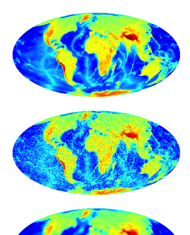
(a) Band-limited signal

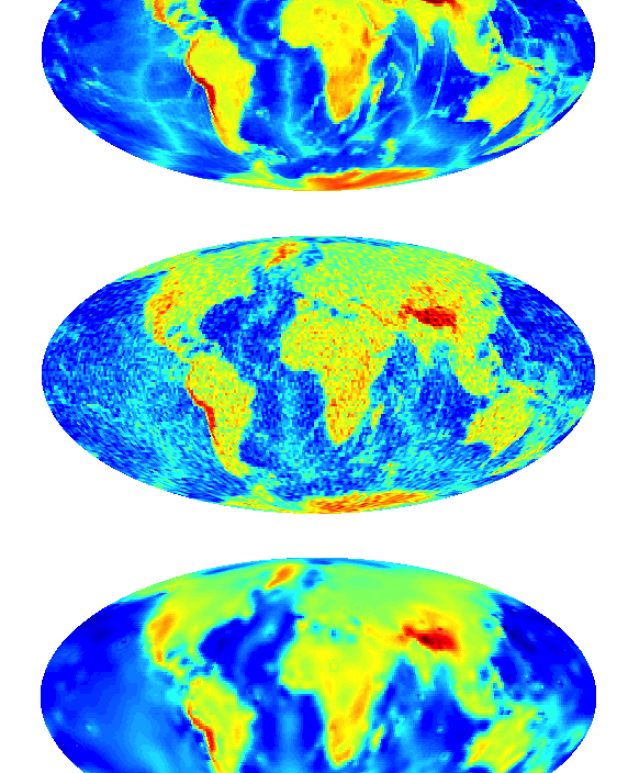
(b) Noisy signal with $\textrm{SNR}(y)=11.8$dB

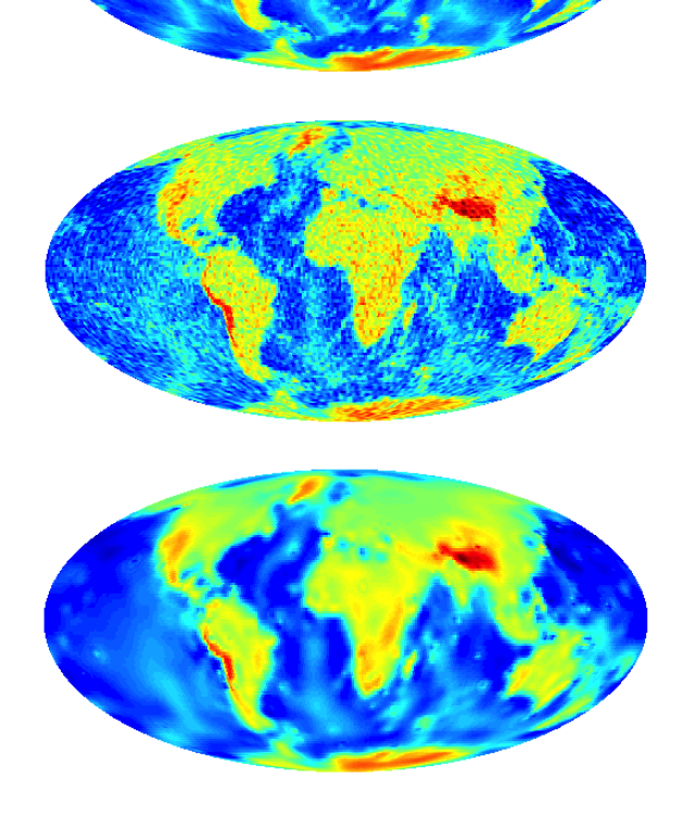
(c) Denoised signal with $\textrm{SNR}(d)=14.66$dB

Figure 5: Wavelet denoising by hard-thresholding, using parameters $\lambda=2$ and $J_{0}=0$ and scale-discretised generating functions.When using needlets and B-spline wavelets, the denoised signals have $\textrm{SNR}(d)=14.68$dB and $14.46$dB respectively. This example is included in S2LET as a documented demo program.

⬇

// Example: Wavelet denoising in C

int lambda = 2, J0 = 0;

// Read a real MW map from a FITS file

char inputfile[100] = "..."

double *f;

int L = s2let_fits_read_mw_bandlimit(file);

s2let_mw_allocate_real(&f, L);

s2let_fits_read_mw_map(f, file, L);

// Perform multiresolution wavelet analysis

double *f_wav, *f_scal;

s2let_axisym_mw_allocate_f_wav_multires_real (&f_wav, &f_scal, lambda, L, J0);

s2let_axisym_mw_wav_analysis_multires_real (f_wav, f_scal, g, lambda, L, J0);

// Threshold the wavelets with a noise model

s2let_axisym_wav_hardthreshold_multires_real (f_wav, threshold, lambda, L, J0);

// Reconstruct the denoised signal

double *f_denoised;

s2let_mw_allocate_real(&f_denoised, L);

s2let_axisym_mw_wav_synthesis_multires_real (f_denoised, f_wav, f_scal, lambda,L,J0);

// Write the denoised signal

char outputfile[100] = "..."

s2let_fits_write_mw_map(outfile,f_denoised,L);

Example 5: Denoising a real signal (MW sampling) in C through hard-thresholding of the wavelet coefficients.

5 Summary

In the era of precision astrophysics and cosmology, large and complex data-sets on the sphere must be analysed at high precision in order to confront accurate theoretical predictions. Scale-discretised wavelets are a powerful analysis technique where spatially localised, scale-dependent signal features of interest can be extracted and analysed. Combined with a sampling theorem, this framework leads to an exact multiresolution wavelet analysis, where signals on the sphere can be reconstructed from their scaling and wavelet coefficients exactly.

We have described S2LET, a fast and robust implementation of the scale-discretised wavelet transform. Although the first public release of S2LET is restricted to axisymmetric wavelets, the generalisation to directional, steerable wavelets will be made available in a future release. The core numerical routines of S2LET are written in C and have interfaces in Matlab, IDL and Java. Both MW and HEALPix pixelisation schemes are supported. In this article we have presented a number of examples to illustrate the ease of use of S2LET for performing wavelet transform of real signals stored as FITS files and to plot scaling and wavelet coefficients on Mollweide projections of the sphere. We have also detailed a denoising example where denoising is performed through simple hard-thresholding in wavelet space. Although only a simple denoising strategy was performed to illustrate the use of the S2LET code, it nevertheless performed very well, highlighting the effectiveness of the scale-discretised wavelet transform on the sphere.

References

- Antoine & Vandergheynst (1998) Antoine, J.-P. & Vandergheynst, P. 1998, J. Math. Phys., 39, 3987
- Antoine & Vandergheynst (1999) Antoine, J.-P. & Vandergheynst, P. 1999, Applied Comput. Harm. Anal., 7, 1
- Baldi et al. (2009) Baldi, P., Kerkyacharian, G., Marinucci, D., & Picard, D. 2009, Annals of Statistics, 37 No.3, 1150
- Barreiro et al. (2000) Barreiro, R. B., Hobson, M. P., Lasenby, A. N., et al. 2000, Mon. Not. Roy. Astron. Soc., 318, 475
- Basak & Delabrouille (2012) Basak, S. & Delabrouille, J. 2012, Mon. Not. Roy. Astron. Soc., 419, 1163
- Cayón et al. (2001) Cayón, L., Sanz, J. L., Martínez-González, E., et al. 2001, Mon. Not. Roy. Astron. Soc., 326, 1243
- Daubechies (1992) Daubechies, I. 1992, Ten Lectures on Wavelets (Society for Industrial and Applied Mathematics)
- Deriaz et al. (2012) Deriaz, E., Starck, J.-L., & Pires, S. 2012, Astron. & Astrophys., 540, A34
- Doroshkevich et al. (2005) Doroshkevich, A. G., Naselsky, P. D., Verkhodanov, O. V., et al. 2005, International Journal of Modern Physics D, 14, 275
- Doroshkevich et al. (2011) Doroshkevich, A. G., Verkhodanov, O. V., Naselsky, P. D., et al. 2011, International Journal of Modern Physics D, 20, 1053
- Driscoll & Healy (1994) Driscoll, J. R. & Healy, D. M. J. 1994, Advances in Applied Mathematics, 15, 202
- Geller et al. (2008) Geller, D., Hansen, F. K., Marinucci, D., Kerkyacharian, G., & Picard, D. 2008, Phys. Rev. D., 78, 123533
- Geller & Marinucci (2010) Geller, D. & Marinucci, D. 2010, ArXiv e-prints
- Górski et al. (2005) Górski, K. M., Hivon, E., Banday, A. J., et al. 2005, ApJ, 622, 759
- Healy et al. (1996) Healy, D., Jr., Rockmore, D., Kostelec, P. J., & Moore, S. S. B. 1996, The Journal of Fourier Analysis and Applications, 9, 341
- Labatie et al. (2012) Labatie, A., Starck, J. L., & Lachièze-Rey, M. 2012, Astron. J., 746, 172
- Lan & Marinucci (2008) Lan, X. & Marinucci, D. 2008, Electronic Journal of Statistics, 2, 332
- Leistedt & McEwen (2012) Leistedt, B. & McEwen, J. D. 2012, IEEE Trans. Sig. Proc., 60
- Marinucci et al. (2008) Marinucci, D., Pietrobon, D., Balbi, A., et al. 2008, Mon. Not. Roy. Astron. Soc., 383, 539
- McEwen et al. (2006) McEwen, J. D., Hobson, M. P., & Lasenby, A. N. 2006, Arxiv preprint astro-ph/0609159
- McEwen et al. (2006) McEwen, J. D., Hobson, M. P., Lasenby, A. N., & Mortlock, D. J. 2006, Mon. Not. Roy. Astron. Soc., 371, L50
- McEwen et al. (2013) McEwen, J. D., Vandergheynst, P., & Wiaux, Y. 2013, in Wavelets and Sparsity XIV, SPIE international symposium on optics and photonics, invited contribution
- McEwen et al. (2007a) McEwen, J. D., Vielva, P., Hobson, M. P., Martínez-González, E., & Lasenby, A. N. 2007a, Mon. Not. Roy. Astron. Soc., 376, 1211
- McEwen et al. (2007b) McEwen, J. D., Vielva, P., Wiaux, Y., et al. 2007b, J. Fourier Anal. and Appl., 13, 495
- McEwen & Wiaux (2011) McEwen, J. D. & Wiaux, Y. 2011, IEEE Trans. Sig. Proc., 59, 5876
- McEwen et al. (2008) McEwen, J. D., Wiaux, Y., Hobson, M. P., Vandergheynst, P., & Lasenby, A. N. 2008, Mon. Not. Roy. Astron. Soc., 384, 1289
- Narcowich et al. (2006) Narcowich, F. J., Petrushev, P., & Ward, J. D. 2006, SIAM J. Math. Anal., 38, 574
- Pietrobon et al. (2008) Pietrobon, D., Amblard, A., Balbi, A., et al. 2008, Phys. Rev. D., 78, 103504
- Pietrobon et al. (2010) Pietrobon, D., Balbi, A., Cabella, P., & Gorski, K. M. 2010, Astrophys. J., 723, 1
- Reinecke (2011) Reinecke, M. 2011, Astron. & Astrophys., 526, A108
- Reinecke & Seljebotn (2013) Reinecke, M. & Seljebotn, D. S. 2013, A&A, 554, A112
- Risbo (1996) Risbo, T. 1996, Journal of Geodesy, 70, 383
- Schmitt et al. (2010) Schmitt, J., Starck, J. L., Casandjian, J. M., Fadili, J., & Grenier, I. 2010, Astron. & Astrophys., 517, A26
- Schröder & Sweldens (1995) Schröder, P. & Sweldens, W. 1995, Computer Graphics Proceedings (SIGGRAPH 95), 161
- Starck et al. (2006a) Starck, J.-L., Moudden, Y., Abrial, P., & Nguyen, M. 2006a, Astron. & Astrophys., 446, 1191
- Starck et al. (2009) Starck, J.-L., Moudden, Y., & Bobin, J. 2009, Astron. & Astrophys., 497, 931
- Starck et al. (2006b) Starck, J.-L., Pires, S., & Réfrégier, A. 2006b, Astron. & Astrophys., 451, 1139
- Sweldens (1996) Sweldens, W. 1996, Appl. Comput. Harmon. Anal., 3, 186
- Sweldens (1997) Sweldens, W. 1997, SIAM J. Math. Anal., 29, 511
- Trapani & Navaza (2006) Trapani, S. & Navaza, J. 2006, Acta Crystallographica Section A, 62, 262
- Vielva et al. (2004) Vielva, P., Martínez-González, E., Barreiro, R. B., Sanz, J. L., & Cayón, L. 2004, Astrophys. J., 609, 22
- Vielva et al. (2006a) Vielva, P., Martínez-González, E., & Tucci, M. 2006a, Mon. Not. Roy. Astron. Soc., 365, 891
- Vielva et al. (2006b) Vielva, P., Wiaux, Y., Martínez-González, E., & Vandergheynst, P. 2006b, New A Rev., 50, 880
- Vielva et al. (2007) Vielva, P., Wiaux, Y., Martínez-González, E., & Vandergheynst, P. 2007, MNRAS, 381, 932
- Wiaux et al. (2005) Wiaux, Y., Jacques, L., & Vandergheynst, P. 2005, Astrophys. J., 632, 15
- Wiaux et al. (2006) Wiaux, Y., Jacques, L., Vielva, P., & Vandergheynst, P. 2006, Astrophys. J., 652, 820
- Wiaux et al. (2008) Wiaux, Y., McEwen, J. D., Vandergheynst, P., & Blanc, O. 2008, Mon. Not. Roy. Astron. Soc., 388, 770
- Wiaux et al. (2007) Wiaux, Y., McEwen, J. D., & Vielva, P. 2007, J. Fourier Anal. and Appl., 13, 477
- Wiaux et al. (2008) Wiaux, Y., Vielva, P., Barreiro, R. B., Martínez-González, E., & Vandergheynst, P. 2008, MNRAS, 385, 939
- Wiaux et al. (2006) Wiaux, Y., Vielva, P., Martínez-González, E., & Vandergheynst, P. 2006, Physical Review Letters, 96, 151303
- Yeo et al. (2008) Yeo, B., Ou, W., & Golland, P. 2008, IEEE Transactions on Image Processing, 17, 283