Solution of the Anderson impurity model via the functional renormalization group

Abstract

We show that the functional renormalization group is a numerically cheap method to obtain the low-energy behavior of the Anderson impurity model describing a localized impurity level coupled to a bath of conduction electrons. Our approach uses an external magnetic field as flow parameter, partial bosonization of the transverse spin fluctuations, and frequency-independent interaction vertices determined by Ward identities. The magnetic field serves also as a regulator for the bosonized spin fluctuations, which are suppressed at large field. We calculate the quasiparticle residue and spin susceptibility in the particle-hole symmetric case and obtain excellent agreement with the Bethe ansatz results for arbitrary coupling.

The Anderson impurity model (AIM) describes a localized impurity in contact with a bath of non-interacting electrons.Anderson61 The model was first introduced in the context of material science for describing the emergence of local moments in metals and has been studied for half a century by various methods.Hewson93 In the past decade, renewed attention has been drawn to the AIM because of its experimental realization in quantum dot systems. Moreover, the solution of the AIM is one of the fundamental steps in the so-called dynamical mean-field theory.Georges96 In practice, this step is often implemented using Wilson’s numerical renormalization group (NRG), which yields numerically controlled results for the thermodynamic and spectral properties.Wilson75 In the 1980s the thermodynamics of the AIM has also been obtained exactly via the Bethe ansatz (BA).Tsvelick83 For later reference, we quote here the BA results for the spin and charge susceptibilities in the particle-hole symmetric case,Zlatic83

$$\pi\Delta{\chi}_{s} = \sqrt{\frac{2}{\pi u}}e^{\pi^{2}u/8}\int_{0}^{\infty}dxe^{-x^{2}/(2u)}\frac{\cos(\pi x/2)}{1-x^{2}},$$ (1a)

$$\pi\Delta{\chi}_{c} = \sqrt{\frac{2}{\pi u}}e^{-\pi^{2}u/8}\int_{0}^{\infty}dxe^{-x^{2}/(2u)}\frac{\cosh(\pi x/2)}{1+x^{2}}.\hskip 14.22636pt$$ (1b)

Here $u=U/(\pi\Delta)$, where $U$ is the interaction between two impurity electrons with opposite spin, and $\Delta$ is the hybridization energy to the conduction bath, in the limit where the latter has infinite bandwidth and constant density of states. For $u\gtrsim 2$ the charge susceptibility ${\chi}_{c}$ becomes exponentially small, while the spin susceptibility ${\chi}_{s}=(2T_{K})^{-1}$ is proportional to the inverse Kondo temperature $T_{K}=\Delta(\pi u/2)^{1/2}e^{-\pi^{2}u/8+1/(2u)}$.

Although Eqs. (1a, 1b) can be confirmed numerically using the NRG, it would be useful to have a numerically cheap method to obtain the correct low-energy physics of the AIM at strong coupling, which is dominated by the exponentially small Kondo temperature. In this work we show that this can be achieved by means of the functional renormalization group (FRG) method.Pawlowski07 ; Kopietz10 ; Metzner12 In the past few years, many authors have studied the AIM using different versions of the FRG,Hedden04 ; Karrasch06 ; Karrasch08 ; Bartosch09 ; Isidori10 ; Jakobs10 ; Freire12 ; Kinza12 but failed in reproducing the correct strong coupling behavior of the AIM. We show that this problem can be solved using a simple truncation of the FRG hierarchy involving only frequency-independent interaction vertices which are fixed by Ward identities (WI), provided that the transverse spin fluctuations are properly bosonized and that the corresponding bosonic self-energy, obtained from a skeleton equation, fulfills the WI.

For simplicity, we focus on the particle-hole symmetric AIM. After integrating out the conduction electrons, we obtain the following Euclidean action for the Grassmann field $d_{\sigma}(\tau)$ describing the localized electron,

$$S=-\int_{\omega}\sum_{\sigma}G_{0,\sigma}^{-1}(i\omega)\bar{d}_{\omega\sigma}d_{\omega\sigma}+U\int_{0}^{1/T}\!\!d\tau\,n_{\uparrow}n_{\downarrow}.$$ (2)

Here $T$ is the temperature (we set $k_{B}=\hbar=1$ and focus on the zero temperature limit below), $\int_{\omega}=T\sum_{\omega}$ denotes summation over fermionic Matsubara frequencies $i\omega$, $n_{\sigma}=\bar{d}_{\sigma}(\tau)d_{\sigma}(\tau)$ represents the number of localized electrons with spin $\sigma=\uparrow,\downarrow$, and $d_{\omega\sigma}=\int_{0}^{1/T}\!d\tau\,e^{i\omega\tau}d_{\sigma}(\tau)$. In the particle-hole symmetric case the inverse bare Green function is $G_{0,\sigma}^{-1}(i\omega)=i\omega+U/2+\sigma H+i\Delta\mathop{\rm sgn}\omega$, where $H$ is the external magnetic field in units of energy.

Our strategy is inspired by the recent work by Edwards and Hewson,Edwards11 who developed a field-theoretical renormalization group approach which yields the correct low-energy physics of the AIM for arbitrary coupling. They noticed that for large magnetic fields the AIM can be studied perturbatively, even for $U\gg\Delta$, as long as $U/H$ is sufficiently small. Following Ref. Edwards11, , let us therefore use the external magnetic field $H$ as a flow parameter for the FRG. Unfortunately, using this cutoff scheme we could not reproduce the strong-coupling physics of the AIM if we formulated the FRG exclusively in terms of fermionic degrees of freedom. The problem is that the resulting fermionic vertices exhibit a rather strong frequency dependence which cannot be neglected. To avoid this problem, we partially bosonize the action (2) by decoupling the interaction in terms of a complex boson field $\chi$ representing transverse spin fluctuations. It turns out to be advantageous, however, to bosonize only a part of the interaction, while retaining a fermionic parametrization for the rest. The reason is that the partial bosonization removes the strong frequency dependence of the interaction vertices only in one particular scattering channel, while the other channels can potentially exhibit strongly frequency-dependent vertices. In order to avoid this phenomenon, one has to find a compromise and retain a part of the interaction in the original fermionic parametrization. Therefore, we write the interaction in Eq. (2) as $Un_{\uparrow}n_{\downarrow}=U_{\parallel}n_{\uparrow}n_{\downarrow}-U_{\bot}s_{+}s_{-}$, where $U=U_{\parallel}+U_{\bot}$, $s_{+}=\bar{d}_{\uparrow}d_{\downarrow}$, and $s_{-}=\bar{d}_{\downarrow}d_{\uparrow}$. Only the transverse part $-U_{\bot}s_{+}s_{-}$ is then bosonized by introducing a complex field $\chi$ via a usual Hubbard-Stratonovich transformation.Bartosch09 ; Isidori10 We choose $U_{\bot}$ such that it vanishes for $H\rightarrow\infty$, and that it reduces to the bare interaction $U$ for $H\rightarrow 0$. Therefore we set $U_{\bot}^{-1}=U^{-1}+R_{H}$ and require $R_{0}=0$ and $R_{\infty}=\infty$. Note that $R_{H}$ plays the role of a regulator for the bosonic sector of the theory which switches on the interaction mediated by transverse spin fluctuations. The proper choice of $R_{H}$ will be discussed in more detail below. In comparison to the renormalization group method developed in Ref. Edwards11, , our FRG approach does not require the introduction of ad hoc counter terms.

It is now straightforward to write down formally exact FRG flow equations for the irreducible vertices of our boson-fermion model.Kopietz10 ; Bartosch09 For our purpose, it is sufficient to neglect the frequency dependence of all vertices with more than two external legs. We also neglect the contribution from charge- and longitudinal spin fluctuations. The resulting flow equation for the fermionic self-energy $\Sigma_{\sigma}(i\omega)$ is shown graphically in Fig. 1; the corresponding analytic expression reads

$$\frac{\partial\Sigma_{\sigma}(i\omega)}{\partial H}=\int_{\omega^{\prime}}\sum_{\sigma^{\prime}}\dot{G}_{\sigma^{\prime}}(i\omega^{\prime}){\Gamma}_{4}^{\bar{d}_{\sigma}\bar{d}_{\sigma^{\prime}}d_{\sigma^{\prime}}d_{\sigma}}$$ (3)

$$+ \int_{\bar{\omega}}\dot{F}_{\bot}(i\bar{\omega})\Gamma_{4}^{\bar{d}_{\sigma}d_{\sigma}\bar{\chi}\chi}+\int_{\omega^{\prime}}\Bigl{[}\dot{G}_{-\sigma}(i\omega^{\prime})F_{\bot}(i\sigma(\omega-\omega^{\prime}))$$

$$\hskip 14.22636pt+\,{G}_{-\sigma}(i\omega^{\prime})\dot{F}_{\bot}(i\sigma(\omega-\omega^{\prime}))\Bigr{]}\Gamma_{3}^{\bar{d}_{\uparrow}d_{\downarrow}\chi}\Gamma_{3}^{\bar{d}_{\downarrow}d_{\uparrow}\bar{\chi}}.$$

The single-scale propagators in our cutoff scheme are

$$\dot{G}_{\sigma}(i\omega) = -\sigma G_{\sigma}^{2}(i\omega),\;\;\dot{F}_{\bot}(i\bar{\omega})=-F_{\bot}^{2}(i\bar{\omega})\partial R_{H}/\partial H,\hskip 8.53581pt$$ (4)

where $G_{\sigma}(i\omega)$ is the exact fermionic Green function and $F_{\bot}(i\bar{\omega})$ is the exact propagator of the spin fluctuation field $\chi$. These propagators can be expressed in terms of the corresponding self-energies $\Sigma_{\sigma}(i\omega)$ and $\Pi_{\bot}(i\bar{\omega})$ via the Dyson equations $G_{\sigma}^{-1}(i\omega)=G_{0,\sigma}^{-1}(i\omega)-\Sigma_{\sigma}(i\omega)$ and $F_{\bot}^{-1}(i\bar{\omega})=U_{\bot}^{-1}-\Pi_{\bot}(i\bar{\omega})$. We denote bosonic Matsubara frequencies by $i\bar{\omega}$. The right-hand side of Eq. (3) depends on the irreducible four-point vertices, ${\Gamma}_{4}^{\bar{d}_{\sigma}\bar{d}_{\sigma^{\prime}}d_{\sigma^{\prime}}d_{\sigma}}$ and $\Gamma_{4}^{\bar{d}_{\sigma}d_{\sigma}\bar{\chi}\chi}$, and on the three-point vertices $\Gamma_{3}^{\bar{d}_{\uparrow}d_{\downarrow}\chi}=\Gamma_{3}^{\bar{d}_{\downarrow}d_{\uparrow}\bar{\chi}}\equiv\gamma$. The superscripts indicate the types of legs attached to the vertices.

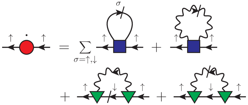
Figure 1: (Color online) FRG flow equation (3) for $\Sigma_{\uparrow}(i\omega)$ (shaded circle). Solid and wavy lines represent full fermion and boson propagators, respectively; slash insertions denote the corresponding single-scale propagators in Eq. (4). The dot on the left represents a derivative with respect to $H$.

Our goal is to derive flow equations for the quasiparticle residue $Z$ and the spin-dependent part $M$ of the fermionic self-energy, defined via the low-energy expansion

$$\Sigma_{\sigma}(i\omega)=U/2-\sigma M+(1-Z^{-1})i\omega+{\cal{O}}(\omega^{2}).$$ (5)

In order to obtain $M$ and $Z$ from the solution of the flow equation (3) we need to know the bosonic self-energy $\Pi_{\bot}(i\bar{\omega})$ and three different vertices: ${\Gamma}_{4}^{\bar{d}_{\sigma}\bar{d}_{\sigma^{\prime}}d_{\sigma^{\prime}}d_{\sigma}}$, $\Gamma_{4}^{\bar{d}_{\sigma}d_{\sigma}\bar{\chi}\chi}$, and $\gamma$. One could write down additional flow equations for these vertices, but these depend on higher order vertices and it is not clear how to truncate this infinite hierarchy. We shall therefore adopt a different strategy which uses WI and skeleton equations to obtain a closed system of flow equations for $M$ and $Z$.

First of all, we note that the three-point vertex can be related to $M$ via the WI

$$\Gamma_{3}^{\bar{d}_{\uparrow}d_{\downarrow}\chi}=\Gamma_{3}^{\bar{d}_{\downarrow}d_{\uparrow}\bar{\chi}}\equiv\gamma=b/(h+u_{\bot}\arctan b),$$ (6)

which can be derived following the work by Koyama and Tachiki.Koyama84 ; Streib13 Here $u_{\bot}=U_{\bot}/(\pi\Delta)$ and $b=h+m$, with $m=M/\Delta$ and $h=H/\Delta$.

Next, let us derive an alternative flow equation for $M$ which does not explicitly involve the four-point vertices. To this end we consider the longitudinal spin-susceptibility $\chi_{\parallel}=\partial s/\partial H$, where $s=\langle n_{\uparrow}-n_{\downarrow}\rangle/2$ is the local magnetic moment, normalized such that $s=1/2$ corresponds to a fully magnetized state. The local moment is then connected to $M$ via the Friedel sum rule,Hewson93

$$\pi s=\arctan(h+m)=\arctan b.$$ (7)

Taking the derivative with respect to $h$ we obtain

$$\partial m/\partial h=\chi_{\parallel}/\rho-1,$$ (8)

where $\rho=[\pi\Delta(1+b^{2})]^{-1}$ is the exact density of states at vanishing energy. To determine $\chi_{\parallel}$ we use the WIHewson93 ; Kopietz10a

$$\chi_{\parallel}/\rho=1/Z+\rho\Gamma_{\bot},$$ (9)

where $\Gamma_{\bot}$ is the exact interaction vertex between two electrons with opposite spin at vanishing frequencies. In our partially bosonized theory we have

$$\Gamma_{\bot}=\gamma^{2}U_{\bot}/[1-U_{\bot}\Pi_{\bot}(0)]+{\Gamma}_{4}^{\bar{d}_{\uparrow}\bar{d}_{\downarrow}d_{\downarrow}d_{\uparrow}}.$$ (10)

But the three-point vertex and the fermionic four-point vertex turn out to be mutually related via a skeleton equation. With the help of standard functional methodsKopietz10 it is straightforward to show that, at finite frequencies,

$$\Gamma_{3}^{\bar{d}_{\uparrow}d_{\downarrow}\chi}(\omega+\bar{\omega},\omega;\bar{\omega}) = 1-\int_{\omega^{\prime}}G_{\downarrow}(i\omega^{\prime})G_{\uparrow}(i\omega^{\prime}+i\bar{\omega})$$ (11)

$$\times{\Gamma}_{4}^{\bar{d}_{\uparrow}\bar{d}_{\downarrow}d_{\downarrow}d_{\uparrow}}(\omega+\bar{\omega},\omega^{\prime};\omega,\omega^{\prime}+\bar{\omega}).$$

Using the above relation to express ${\Gamma}_{4}^{\bar{d}_{\uparrow}\bar{d}_{\downarrow}d_{\downarrow}d_{\uparrow}}$ in terms of $\Gamma_{3}^{\bar{d}_{\uparrow}d_{\downarrow}\chi}\equiv\gamma$, we find for the longitudinal susceptibilityfootnoteskeleton

$$\frac{{\chi}_{\parallel}}{\rho}=\frac{1}{Z}+\frac{1}{1+b^{2}}\frac{b}{\arctan b}\left[\frac{b}{h}-\frac{1}{Z}\right],$$ (12)

where we have used the WI (6) to eliminate the vertex $\gamma$. Substituting the expression (12) into Eq. (8), we obtain a flow equation for $m$ which depends only on the self-energy parameters $m$ and $Z$.

Finally, to close our system of flow equations we approximate the bosonic self-energy $\Pi_{\bot}(i\bar{\omega})$, appearing implicitly in Eq. (3), by

$$\pi\Delta\Pi_{\bot}(i\bar{\omega})=\gamma P_{\bot}(|\bar{\omega}|/(Z\Delta),b\mathop{\rm sgn}\bar{\omega}),$$ (13)

where the dimensionless function

$$P_{\bot}(x,b)=\frac{\ln[1+x/(1-ib)]}{(x-2ib)(1+x/2-ib)}-\frac{2i\arctan b}{x-2ib}$$ (14)

is obtained from the skeleton equationBartosch09 for $\Pi_{\bot}(i\bar{\omega})$. The prefactor in Eq. (13) is determined by demanding that $\Pi_{\bot}(0)$ satisfy the WIKoyama84 ; Edwards11

$$\Pi_{\bot}(0)/[1-U_{\bot}\Pi_{\bot}(0)]\equiv\chi_{\bot}=s/H$$ (15)

relating the transverse spin-susceptibility $\chi_{\bot}$ to the local moment $s$. Using the Friedel sum rule (7) it is easy to see that our expression (12) for the longitudinal susceptibility is consistent with Eq. (15) for $\chi_{\bot}$, in the sense that for $H\rightarrow 0$ both susceptibilities approach the same limit $\chi_{s}$. We point out that Eqs. (6) and (15) imply that $a\equiv[1-U_{\bot}\Pi_{\bot}(0)]=h/(h+u_{\bot}\arctan b)>0$, which guarantees that there is no magnetic instability.

We have now obtained a closed system of flow equations for $m$ and $Z$. For simplicity, we also expand the function $P_{\bot}(x,b)$ in Eq. (13) to linear order in $x$, which is consistent with the low-energy expansion (5) in the fermionic sector. After straightforward algebra we arrive at the flow equation $h\partial Z/\partial h=\eta Z$ for the quasiparticle residue $Z$, with

$$\eta = hZ\gamma^{2}u_{\bot}{\rm Im}\int_{0}^{\infty}\frac{dx}{(1-ib+x)^{2}}\frac{c}{(a+cx)^{2}}$$ (16)

$$+ hZ\gamma^{2}u_{\bot}^{2}\frac{\partial r}{\partial h}{\rm Re}\int_{0}^{\infty}\frac{dx}{(1-ib+x)}\frac{2c}{(a+cx)^{3}}.$$

Here $r=\pi\Delta R_{H}$ is the dimensionless bosonic regulator, and

$$c=(u_{\bot}\gamma)(2ib)^{-1}\left[(1-ib)^{-2}-\arctan b/b\right].$$ (17)

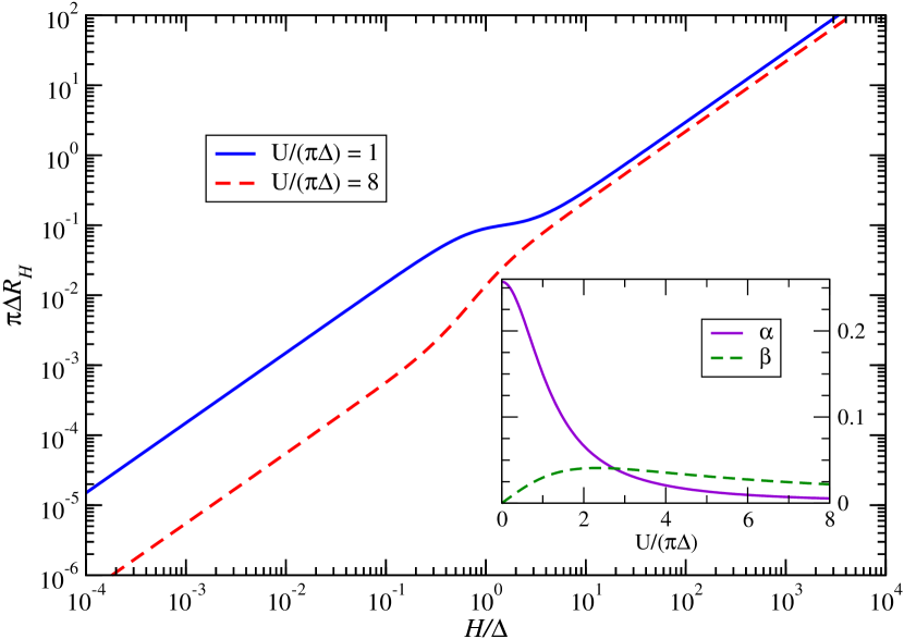
Figure 2: (Color online) Bosonic regulator $r=\pi\Delta R_{H}$ as a function of the magnetic field $h=H/\Delta$, for $U/(\pi\Delta)=1$ (solid line) and $U/(\pi\Delta)=8$ (dashed line). The regulator is linear in $h$ at small and large $h$, with a change in slope from $\alpha$ ($h\lesssim 1$) to $\beta$ ($h\gtrsim 1$). The inset shows the $U$-dependence of $\alpha$ and $\beta$.

The above system of flow equations can be easily solved numerically once the regulator $r=\pi\Delta R_{H}$ has been specified. The simplest choice of a linear magnetic field dependence of the bosonic regulator ($r\propto h$, in analogy with the regulator in the fermionic sector) does not lead to satisfactory results. Instead, we found that the best optimization is obtained with a regulator of the form

$$r=(\alpha-\beta)h/(1+h^{2})+\beta h,$$ (18)

which is linear in $h$ both for small and large $h$, but exhibits a change in slope from $\alpha$ to $\beta$ at $h\approx 1$, as shown in Fig. 2. The specific form of our regulator, in Eq. (18), is of course only one possible choice. Any other functional form which switches between two slopes as a function of the magnetic field yields practically identical results: We have checked this explicitly using the alternative function $r=(\alpha-\beta)\arctan h+\beta h$. Comparing our FRG results at weak coupling, $U\ll\Delta$, with the known perturbative expansion for $Z$ and $\chi_{s}$, we also realized that the coefficients $\alpha$ and $\beta$ are weakly dependent functions of the dimensionless bare interaction $u=U/(\pi\Delta)$. Their functional dependence is well described by rational functions of low degree. Hence, we introduce the following ansatz,

$$\alpha=\alpha_{0}/(\alpha_{2}+u^{2}),\;\;\;\beta=\beta_{1}u/(\beta_{2}+u^{2}),$$ (19)

where the four parameters $\alpha_{0}$, $\alpha_{2}$, $\beta_{1}$, and $\beta_{2}$ can be determined by matching the FRG results for $Z$ and $\chi_{s}$ at weak coupling (e.g., for $u=0.1$) with the corresponding values obtained in perturbation theory at ${\cal O}(u^{2})$, and by imposing that the Wilson ratio $R$ is equal to 2 for two values of $u$ in the Kondo regime (e.g., we impose $R=2$ for $u=4$ and $u=8$). Note that in the AIM the expression for the Wilson ratio reads

$$R\equiv\frac{{\chi}_{s}(U)/{\chi}_{s}(0)}{Z^{-1}(U)/Z^{-1}(0)}=\pi\Delta{\chi}_{s}Z=\frac{2{\chi}_{s}}{{\chi}_{s}+{\chi}_{c}},$$ (20)

where the last equality follows from the Yamada-Yosida WI.Kopietz10a ; Yamada75 At large $U$, charge fluctuations are strongly suppressed and the low-energy physics of the AIM is effectively the same as in the Kondo model. In this regime the charge susceptibility ${\chi}_{c}$ is then negligible and the Wilson ratio takes the Kondo-model value $R=2$. For the parametrization of $\alpha$ and $\beta$ in Eq. (19), we find $\alpha_{0}\approx 0.36$, $\alpha_{2}\approx 1.4$, $\beta_{1}\approx 0.19$, and $\beta_{2}\approx 5.4$. The $U$-dependence of $\alpha$ and $\beta$ is shown in the inset of Fig. 2. As a final remark, we note that in principle it should be possible to fix the interaction dependence of $\alpha$ and $\beta$ entirely from a fit to the weak coupling expansion, but we found that this fit is numerically unstable. Instead, the requirement that at strong coupling the Wilson ratio equals 2 for two (arbitrary) values of the interaction yields numerically stable constraints on the regulator. More complicated regulators, involving more parameters, are of course possible, but our four-parameter regulator defined in Eqs. (18) and (19) is the simplest one that is able to interpolate between some known weak- and strong-coupling behaviors: The perturbative weak-coupling expansion, and the asymptotic value of the Wilson ratio, which are both a priori accessible even in more complex models for which no exact solution is available.

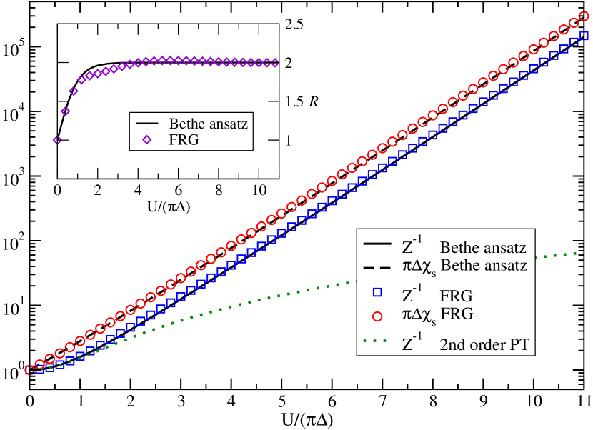
Figure 3: (Color online) Quasiparticle residue $Z^{-1}$ and spin susceptibility $\chi_{s}$ as functions of $U/(\pi\Delta)$ for $H=0$. The FRG results for $Z^{-1}$ (squares) and $\chi_{s}$ (circles) are compared with the corresponding BA results (solid and dashed lines, respectively). The dotted line represents $Z^{-1}$ within second-order perturbation theory. The inset shows the FRG (diamonds) and BA (solid line) results for the Wilson ratio $R$.

Having fixed the bosonic regulator, we can now solve the flow equations numerically, with minimal computational cost. Choosing the initial magnetic field $H_{0}$ sufficiently large, we may use as initial conditions for $M$ and $Z$ the Hartree-Fock values $M_{0}=U/2$ and $Z_{0}=1$, which are exact in the limit $H_{0}\to\infty$. The FRG results for $Z$ and $\chi_{s}$, at $H=0$, are shown in Fig. 3. The remarkable agreement of our approach with the BA results shows that the present FRG truncation, supplied with exact WI, is indeed able to capture the exponentially small Kondo scale.

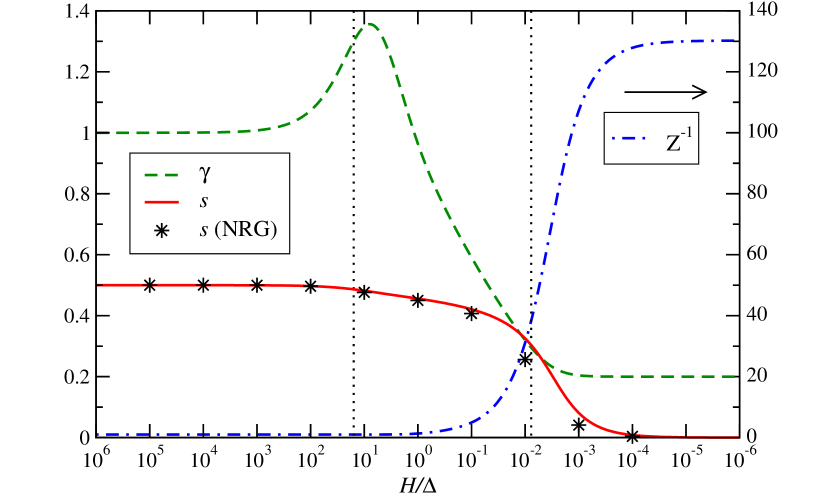
Figure 4: (Color online) Quasiparticle residue $Z^{-1}$ (dot-dashed line, right scale), magnetic moment $s$ (solid line), and three-point vertex $\gamma$ (dashed line) as functions of $H$ for $U/(\pi\Delta)=5$, calculated with FRG. The vertical dotted lines indicate the crossover scales $H=U$ and $H=Z\Delta\approx T_{K}$. Symbols denote the corresponding NRG results for $s$.

In Fig. 4 we show, for $u=U/(\pi\Delta)=5$, the magnetic field dependence of $Z$, $s$, and $\gamma$. In the magnetization curve $s(H)$ one can clearly identify the two energy scales characterizing the strong coupling regime of the AIM, namely the bare interaction $U$ and the width $Z\Delta\approx T_{K}$ of the Kondo resonance. Indeed, reducing the external magnetic field $H$ from a large initial value, at $H\approx U$ we observe a slow logarithmic decrease in the magnetic moment from the initial value $s=1/2$. This regime, where $U\gtrsim H\gtrsim T_{K}$, corresponds to the localized moment regime:Tsvelick83 Here $s(H)$ behaves as a rational function of $\ln(H/T_{K})$. The decrease in $s$ becomes then faster when $H\approx Z\Delta$ (Kondo regime), until the magnetization vanishes linearly, as $s(H)=\chi_{s}H$, for $H\ll Z\Delta$. The presence of two different energy scales is also reflected in the non-monotonic behavior of the three-point vertex $\gamma(H)$. Starting from the bare value $\gamma=1$ at large $H$, the vertex becomes initially larger than unity for $H\approx U$ and later decreases again, approaching (at strong coupling) the value $1/u<1$ for $H\lesssim Z\Delta$.

In summary, we have developed an FRG approach to the AIM which uses the external magnetic field $H$ as a physical flow parameter, and where the fermionic interaction $U$ is partially decoupled via a bosonic field describing transverse spin fluctuations. The latter are controlled by an $H$-dependent regulator, which suppresses the transverse spin fluctuations at large $H$. We have truncated the FRG flow equations keeping only frequency-independent vertices and expanding the fermionic and bosonic self-energies to linear order in frequency. With the help of WI we have expressed all the relevant vertices in terms of self-energy parameters, thereby avoiding further approximations in the flow equations for the vertices. Comparing our results with the BA solution, we have shown that the present approach is able to reproduce the exponential $U$-dependence of the Kondo scale. Moreover, the use of the magnetic field as a flow parameter gives access to the $H$-dependence of physical observables such as the local magnetization. Possible extensions of the present method include finite temperature calculations, the study of the non-symmetric AIM, and a generalization of our approach to non-equilibrium. In each of these cases, one needs to generalize the WI used in this paper to the relevant situation. At finite temperatures, and in the non-symmetric AIM, the modified WI can be derived using the same functional methods used here.Kopietz10 For systems out of equilibrium, instead, the work by OguriOguri01 shows that it is possible to generalize the WI for the AIM to non-equilibrium using the Keldysh diagrammatic formalism.

We thank A. C. Hewson for useful discussions and for making his unpublished notes on the AIM available to us. This work was supported by the DFG via FOR 723.

References

- (1) P. W. Anderson, Phys. Rev. 124, 41 (1961).
- (2) A. C. Hewson, The Kondo Problem to Heavy Fermions, (Cambridge University Press, Cambridge, 1993).
- (3) A. Georges, G. Kotliar, W. Krauth, and M. Rozenberg, Rev. Mod. Phys. 68, 13 (1996).
- (4) K. G. Wilson, Rev. Mod. Phys. 47, 773 (1975); R. Bulla, T. Costi, and T. Pruschke, ibid. 80, 395 (2008).
- (5) A. M. Tsvelick and P. B. Wiegmann, Adv. Phys. 32, 453 (1983).
- (6) V. Zlatić and B. Horvatić, Phys. Rev. B 28, 6904 (1983).
- (7) J. M. Pawlowski, Ann. Phys. 322, 2831 (2007).
- (8) P. Kopietz, L. Bartosch, and F. Schütz, Introduction to the Functional Renormalization Group, (Springer, Berlin, 2010).
- (9) W. Metzner, M. Salmhofer, C. Honerkamp, V. Meden, and K. Schönhammer, Rev. Mod. Phys. 84, 299 (2012).
- (10) R. Hedden, V. Meden, T. Pruschke, and K. Schönhammer, J. Phys.: Cond. Mat. 16, 5279 (2004).
- (11) C. Karrasch, T. Enss, and V. Meden, Phys. Rev. B 73, 235337 (2006).
- (12) C. Karrasch, R. Hedden, R. Peters, T. Pruschke, K. Schönhammer, and V. Meden, J. Phys.: Cond. Mat. 20, 345205 (2008).
- (13) L. Bartosch, H. Freire, J. J. R. Cardenas, and P. Kopietz, J. Phys.: Cond. Mat. 21, 305602 (2009).
- (14) A. Isidori, D. Roosen, L. Bartosch, W. Hofstetter, and P. Kopietz, Phys. Rev. B 81, 235120 (2010).
- (15) S. G. Jakobs, M. Pletyukhov, and H. Schoeller, Phys. Rev. B 81, 195109 (2010).
- (16) H. Freire and E. Corrêa, J. Low Temp. Phys. 166, 192 (2012).
- (17) M. Kinza, J. Ortloff, J. Bauer, and C. Honerkamp, arXiv:1210.0763.
- (18) K. Edwards and A. C. Hewson, J. Phys.: Condens. Matter 23, 045601 (2011).
- (19) T. Koyama and M. Tachiki, Prog. Theor. Phys. Supplement 80, 108 (1984).
- (20) S. Streib, A. Isidori, and P. Kopietz, unpublished.
- (21) P. Kopietz, L. Bartosch, L. Costa, A. Isidori, and A. Ferraz, J. Phys. A: Math. Theor. 43, 385004 (2010).
- (22) Since we are neglecting the frequency dependence of all vertices, we need to introduce a correction factor in Eq. (11). This can be fixed by demanding that, for , in Eq. (12) approach the same limit as in Eq. (15).
- (23) K. Yamada, Prog. Theor. Phys. 53, 970 (1975); K. Yosida and K. Yamada, ibid. 53, 1286 (1975); K. Yamada, ibid. 54, 316 (1975).
- (24) A. Oguri, Phys. Rev. B 64, 153305 (2001).