Numerical approximation of conditionally invariant measures via Maximum Entropy

Abstract

It is well known that open dynamical systems can admit an uncountable number of (absolutely continuous) conditionally invariant measures (ACCIMs) for each prescribed escape rate. We propose and illustrate a convex optimisation based selection scheme (essentially maximum entropy) for gaining numerical access to some of these measures. The work is similar to the Maximum Entropy (MAXENT) approach for calculating absolutely continuous invariant measures of nonsingular dynamical systems, but contains some interesting new twists, including: (i) the natural escape rate is not known in advance, which can destroy convex structure in the problem; (ii) exploitation of convex duality to solve each approximation step induces important (but dynamically relevant and not at first apparent) localisation of support; (iii) significant potential for application to the approximation of other dynamically interesting objects (for example, invariant manifolds).

1 Introduction

Classical dynamical systems concerns the existence and stability of invariant sets under the action of a transformation $T:X\to X$. Depending on the setting, $X$ may be a measure space, a topological space (with or without a metric structure), a differentiable manifold, a Banach space, and so on. In each case, orbits defined by iterative application of $T$ remain in $X$. For an open dynamical system, $T$ is defined only on a subset $A\subsetneq X$, and there are $x\in A$ for which $T(x)\notin A$. Such $x$ are said to escape.

Open dynamical systems may be studied in their own right (the paper of Demers and Young [12] gives a summary of important questions), or may be used to study metastable states in closed dynamical systems. In the latter case, a subset $A\subset X$ is metastable if $T(A)\setminus A$ is in some sense small relative to $A$. Work on making this precise dates at least to 1979, when Pianigiani & Yorke [22] introduced conditionally invariant measures (see Section 1.2 below) and used them to study metastability in expanding interval maps. More recently, Homburg and Young [19] made productive use of conditionally invariant measures to analyse intermittent behaviour near saddle-node and boundary crisis bifurcations in unimodal families. Many authors have continued to obtain results connecting escape rates and metastable behaviour of closed systems; see, for example, [1, 2, 13, 16, 18, 20].

One of the interesting challenges is to find conditionally invariant measures which model the escape statistics of orbits distibuted according to some “natural” initial measure $m$ on $A$. In closed dynamical systems there may exist a unique ergodic invariant measure $\mu$ which is absolutely continuous (AC) with respect to $m$. Via Birkhoff’s ergodic theorem, such $\mu$ describe the orbit distibution of large sets of initial conditions. By contrast, an open system may support uncountably many AC conditionally invariant measures (ACCIMs) [12, Theorem 3.1], so ascribing dynamical significance on the basis of absolutely continuity alone does not make sense. Recently, progress has been made in a variety of settings, identifying ACCIMs whose densities arise as eigenfunctions of certain quasicompact conditional transfer operators acting on suitable Banach spaces. Such ACCIMs may be considered “natural” (see [12] for discussion), giving a well-defined escape rate from $A$. See, for example, [6] for dynamics on Markov towers; [9, 10] for interval maps modelled by Young towers; [7, 8] for expanding circle maps and subshifts of finite type; [21] for interval maps with BV potentials. Extending these techniques to higher-dimensional settings such as billiards and Lorentz gas is an area of much current interest [11].

This chapter develops a new class of computational methods for the explicit approximation of conditionally invariant probability measures on $A$. Our ideas use convex optimisation: the criteria for conditional invariance are expressed as a sequence of moment conditions over $L^{1}$ (integration against a suitable set of $L^{\infty}$ test functions), and the principle of maximum entropy (MAXENT) is used to select (convergent) sequences of approximately conditionally invariant measures. The entropy maximisation is solved via standard convex duality techniques, although attainment in the dual problem may necessitate a non-obvious (but dynamically meaningful) reduction of the domain on which the maximisation is done. The required steps are achievable for piecewise constant test functions (similar in spirit to Ulam’s method [15] but with a completely different mathematical foundation). The chapter is structured as follows: first, we introduce notation for our study of open systems and formulate the ACCIM problem (and its uncountable multiplicity of solutions) via conditional transfer operators; next, the MAXENT problem is set up and analysed; the Ulam-style test functions are introduced in Section 3, and the domain reduction and some numerical examples are given to illustrate the method; we finish with some concluding remarks.

1.1 Nonsingular open dynamical systems

Let $(X,m)$ be a measure space. We consider the dynamics generated by a transformation on a subset of $X$ which fails to be forward invariant; such a dynamical system is called open and may or may not support any recurrent behaviour. Let $A\subsetneq X$ be measurable and let $T:A\rightarrow X$ be a measurable transformation where

• $H_{0}:=T(A)\setminus A$ is a measurable subset of $X$ (called the hole); and

• $m(A\cap T^{-1}H_{0})>0$; and

• $m(E)>0$ whenever $m(T^{-1}E)>0$ and $E$ is a measurable subset of $X$; and

• $T$ is locally finite-to-one (for each $x\in A$, $T^{-1}(x)=\{x_{-1}\in A~{}:~{}T(x_{-1})=x\}$ is either empty or finite).

Definition 1.

Let $m|_{A}$ denote the restriction of the measure $m$ to $A$. We call $(T,A,m|_{A})$ satisfying the above conditions a nonsingular open dynamical system.

Notice that $T(x)$ is defined only for $x\in A$, and the “hole” $H_{0}$ can be used to define a survival time for each $x\in A$:

$$\tau(x):=\left\{\begin{array}[]{ll}n&\mbox{if~{}}x,T(x),\ldots T^{n}(x)\in A~{}\mbox{and}~{}T^{n+1}(x)\in H_{0}\\ \infty&\mbox{if~{}}T^{k}(x)\in A\;\forall k\in\mathbb{Z}_{+}.\end{array}\right.$$

When $\tau(x)=n<\infty$, $T^{n}(x)\in H_{1}:=A\cap T^{-1}(H_{0})$ and such orbits of $T$ terminate at time $\tau(x)+1$. Only those $x$ for which $\tau(x)=\infty$ can exhibit recurrent behaviour.

For all that follows it is convenient to decompose $A$ into invariant and transient parts. Define:

• the $n$ step survivor set as

  $$A_{n}:=\{x\in A~{}:~{}\tau(x)\geq n\}=\left\{x~{}:~{}x,T(x),\ldots,T^{n}(x)\in A\right\}=\cap_{k=0}^{n}T^{-k}A.$$

• $A_{\infty}:=\cap_{n\geq 0}A_{n}$

• $H_{n}:=A_{n-1}\setminus A_{n}=\{x~{}:~{}\tau(x)=n-1\}$ for $1<n<\infty$

Notice that if $x\in H_{n}$ then $T^{k}(x)\in H_{n-k}$ for $0<k\leq n$. The orbit of $x$ “falls into the hole” at time $n$ (escapes) and is lost to the system thereafter. As well as escape from $A$, we need to account for the possibility that backwards orbits may not be defined ($T:A_{1}\rightarrow A$ may not be onto). Since some $x\in A$ may have no preimages in $A$, define the following subsets of $A$:

• $K_{0}:=\{x~{}:~{}A\cap T^{-1}x=\emptyset\}$

• $K_{n}:=\{x~{}:~{}\emptyset\neq(A\cap T^{-n}(x))\subset K_{0}\}=\{x~{}:~{}\min\{k~{}:~{}A\cap T^{-k}x=\emptyset\}=n+1\}$

• $K_{\infty}:=\{x_{0}~{}:~{}\mbox{there is no sequence $\{x_{-n}\}_{n=1}^{\infty}$ such that $T(x_{-n})=x_{-(n-1)}$, $n>0$}\}$

• $H_{\infty}:=\cup_{n>0}(H_{n}\setminus K_{\infty})$

Points in $K_{\infty}$ are ‘backward transient’, while points in $H_{\infty}$ are ‘forward transient’. Lemma 1 contains some facts about the action of $T$ on the various sets $H_{n},K_{n}$. The reader may easily verify that

• $A_{0}=A$ and $T(A_{n})\subseteq A_{n-1}$

• $H_{n}\cap H_{m}=\emptyset$ if $n\neq m$, $H_{n}\subseteq A_{n-1}$ and $H_{n}\cap A_{n}=\emptyset$

• $T(H_{n})\subseteq H_{n-1}$

• $A\cap T^{-1}(K_{n})\subseteq\cup_{m<n}K_{m}$ and $K_{n+1}\subseteq T(K_{n})$

• $\cup_{n=0}^{\infty}K_{n}\subseteq K_{\infty}$, and the union on the left may be finite or infinite (or even the emptyset if $T$ is onto $A$)

Any of the containments above may be strict. In order to avoid unduly messy formulas, from this point on we will generally assume the range of the map $T^{-1}$ is restricted to $A$.

Lemma 1.

Let $(T,A,m|_{A})$ be a nonsingular open dynamical system. If $\Omega:=A_{\infty}\setminus K_{\infty}$ then $A$ admits the disjoint decomposition $A=K_{\infty}\cup\Omega\cup H_{\infty}$ and

1. $T^{-1}(\cup_{n\geq 0}K_{n})\subseteq\cup_{n\geq 0}K_{n}\pmod{m|_{A}}$;

2. $T(\Omega)=\Omega$;

3. $T:(H_{n}\setminus K_{\infty})\to(H_{n-1}\setminus K_{\infty})$ is onto and nonsingular (with respect to the obvious restrictions of $m$);

4. $K_{\infty}=\cup_{n=0}^{\infty}K_{n}$.

Proof.

(a) Note that $T^{-1}K_{n}\subseteq\cup_{m<n}K_{m}$ (for each $n>0$) and $T^{-1}K_{0}=\emptyset$.
(b) If $x\in\Omega$ then $x\in A_{\infty}$ so $T^{n}(x)\in A_{\infty}$. Thus $\Omega$ is the set of points whose future orbit is contained in $A$ and has at least one backwards orbit in $A$.
(c) Let $x\in H_{n-1}\setminus K_{\infty}$. Then there is a sequence $\{x_{-k}\}_{k=1}^{\infty}$ such that $T(x_{-k})=x_{-(k-1)}$ and $T(x_{-1})=x$. Clearly $x_{-1}\in H_{n}\setminus K_{\infty}$.
(d) First, suppose that $x\notin\cup_{n\geq 0}K_{n}$. Then $x\notin K_{0}$ so $\emptyset\neq T^{-1}x$. If $T^{-1}x\subseteq\cup_{n\geq 0}K_{n}$ then there are $N_{1},\ldots,N_{j}$ such that $T^{-1}x\subseteq K_{N_{1}}\cup\cdots\cup K_{N_{j}}$. Putting $N=1+\max\{N_{1},\ldots,N_{j}\}$ one has $x\in K_{N}$, a contradiction. Thus, there is at least one $x_{-1}\in T^{-1}x$ such that $x_{-1}\notin\cup_{n\geq 0}K_{n}$. The proof is completed by induction. ∎

Example 1.

Let $X=\mathbb{R}^{2}$, $A=[0,1]^{2}$ and $T(x,y)=(2x,1/2y)$. Then $H_{n}=(2^{-n},2^{-(n-1)}]\times[0,1]$, $A_{\infty}=\{0\}\times[0,1]$. On the other hand, $K_{n}=[0,1]\times(2^{-(n+1)},2^{-n}]$, so $K_{\infty}=[0,1]\times(0,1]$. The “recurrent set” $A_{\infty}\setminus K_{\infty}=\{(0,0)\}$ is a fixed point (so genuinely recurrent), and $A_{\infty}\cap K_{\infty}=\{0\}\times(0,1]$ is part of the stable manifold to $(0,0)$. Notice that $H_{\infty}=(0,1]\times\{0\}$ is part of the unstable manifold to $(0,0)$.

1.2 Escape, conditionally invariant measures and their supports

We now make precise the notion of escape rates and establish some important connections with conditionally invariant measures.

Definition 2.

The escape rate of a probability measure $m_{0}$ on $A$ is

$$\rho_{m_{0}}:=\lim_{n\to\infty}-\frac{1}{n}\log m_{0}(A_{n})=\lim_{n\to\infty}-\frac{1}{n}\log m_{0}\{x~{}:~{}\tau(x)\geq n\}$$

(when such a limit exists). The open system $(T,A,m|_{A})$ will satisfy the escape hypothesis iff

$$m(A_{\infty})=0.$$ (1)

Clearly, if there is an escape rate $\rho_{m}>0$ then (1) holds.

Definition 3.

A probability measure $\mu$ on $A$ is a conditionally invariant measure (CIM) iff there is $\alpha\in(0,1)$ such that

$$\mu(T^{-1}E)=\alpha\,\mu(E)\qquad\forall\mbox{measurable~{}}E\subseteq A.$$

Note that if $\mu$ is a CIM then

$$\mu\{\tau\geq n\}=\mu(A_{n})=\mu(A\cap T^{-1}A_{n-1})=\alpha\,\mu(A_{n-1})=\cdots=\alpha^{n}\,\mu(A)=\alpha^{n}.$$

Thus $\rho_{\mu}=-\log\alpha$ and $\mu\{x~{}:~{}\tau(x)\geq n\}=\mu(A_{n})=e^{-\rho_{\mu}\,n}$, so that initial conditions distributed according to $\mu$ display geometric escape. Provided $H_{\infty}\neq\emptyset$, Lemma 1(c) implies the existence of at least one backwards semi-orbit $\{x_{-k}\}_{k\geq 0}$ (with $T(x_{-k})=x_{-(k-1)}$). Demers and Young [12] point out that a CIM can be obtained as $(1-\alpha)\sum_{k=0}^{\infty}\alpha^{k}\delta_{x_{-k}}$. However, such CIMs describe only a single orbit, and it remains an interesting challenge to find conditionally invariant measures which model the escape statistics of the “natural” initial measure $m|_{A}$.

The domain decomposition of Lemma 1 and the following Lemma 2 reveal that that $A$ decomposes into three pieces:

1. a backwards transient part $K_{\infty}$ which cannot support any CIMs, but includes any local basins of attraction (we will later identify numerically certain parts of $K_{\infty}$ and exclude them for computational reasons). The intuition behind this fact is that the lack of preimages of points in $K_{\infty}$ means there is no way to “replenish” mass which is lost to the hole;
   

2. an envelope $\Omega=A_{\infty}\setminus K_{\infty}$ for the “recurrent” piece which can support invariant measures, but not CIMs; and
   

3. a transient part $H_{\infty}$ which is the place to look for CIMs (and includes any local unstable manifolds).

Lemma 2.

Let $(T,A,m|_{A})$ be a nonsingular open dynamical system and let $\Omega$, $K_{\infty}$ and $H_{\infty}$ be as defined previously. Then

1. if $\mu$ is an invariant or conditionally invariant measure on $A$ then $\mu(K_{n})=0$ for all $n$ (and $\mu(K_{\infty})=0$);

2. if $\mu$ is an invariant measure then $\mu(H_{\infty})=0$;

3. if $\mu$ is a conditionally invariant measure then $\mu(\Omega)=0$.

Proof.

(a) Suppose that $\mu\circ T^{-1}=\alpha\,\mu$ for some $\alpha\in(0,1]$. Then

$$\alpha^{n+1}\,\mu(K_{n})=\mu\circ T^{-(n+1)}(K_{n})=\mu\circ T^{-1}(T^{-n}K_{n})\leq\mu(T^{-1}K_{0})=\mu(\emptyset)=0.$$

By part (d) of Lemma 1, $\mu(K_{\infty})=\mu(\cup_{n}K_{n})\leq\sum_{n}\mu(K_{n})=0$.
(b) If $\mu$ is an invariant measure and $\mu(H_{n})>0$ then by the Poincaré recurrence theorem almost every $x\in H_{n}$ recurs to $H_{n}$ infinitely often. But if $x\in H_{n}$ then $\{k>n~{}:~{}T^{k}x\in H_{n}\}=\emptyset$, so $\mu(H_{n})=0$. It follows that $\mu(\cup H_{n})=0$ and hence $\mu(H_{\infty})=0$.
(c) By Lemma 1 (b), $\Omega\subseteq T^{-1}(T(\Omega))\subseteq T^{-1}\Omega$ so that

$$\mu(\Omega)\leq\mu\circ T^{-1}(\Omega)=\alpha\,\mu(\Omega)<1\,\mu(\Omega).$$

Hence $\mu(\Omega)=0$. ∎

Example 1 revisited. Let $X=\mathbb{R}^{2}$, $A=[0,1]^{2}$ and $T(x,y)=(2x,1/2y)$. Since $\Omega=\{0\}$, $K_{\infty}=[0,1]\times(0,1]$ and $H_{\infty}=(0,1]\times\{0\}$, the only invariant measure is concentrated on the fixed point at $0$ and all CIMs are concentrated on $H_{\infty}$ (the unstable manifold to $(0,0)$).

Remark 1.

As suggested already, a discrete variant of the set $K_{\infty}$ arises naturally in the numerical methods described below. When $T$ is countable-to-one, it can occur that $K_{\infty}\neq\cup_{n}K_{n}=:K^{\prime}_{\infty}$, but this does not alter the result of Lemma 2(a).

1.3 Conditional transfer operators and the multiplicity of ACCIMs

We complete the introduction by characterising CIMs as eigenvectors of certain conditional transfer operators. This provides a concrete mathematical setting for the approximation algorithms, and gives a useful technical tool for establishing the existence of absolutely continuous CIMs.

For each $k\geq 0$ put $m_{k}=m|_{A_{k}}$ (so that $m_{0}=m|_{A}$). Then $T:(A_{k+1},m_{k+1})\to(A_{k},m_{k})$ is a nonsingular transformation, so that $m_{k+1}\circ T^{-1}\ll m_{k}$ and a conditional Frobenius–Perron operator $\mathcal{L}_{k}:L^{1}(A_{k+1};m_{k+1})\to L^{1}(A_{k};m_{k})$ can be defined in the usual manner:

$$\mathcal{L}_{k}f=\frac{d}{dm_{k}}([f\,m_{k+1}]\circ T^{-1}).$$

Dual to $\mathcal{L}_{k}$ is the (conditional) Koopman operator $U_{k}:L^{\infty}(A_{k};m_{k})\to L^{\infty}(A_{k+1};m_{k+1})$ with the action

$$U_{k}\psi=\psi\circ T.$$

The relation

$$\int_{A_{k}}(\mathcal{L}_{k}\,\varphi)\,\psi\,dm_{k}=\int_{A_{k+1}}\varphi\,U_{k}\psi\,dm_{k+1}$$ (2)

is automatic for $\varphi\in L^{1}(A_{k+1};m_{k+1}),\psi\in L^{\infty}(A_{k};m_{k})$. In particular, for any $\varphi\in L^{1}(A;m_{0})$ and $\psi\in L^{\infty}(A;m_{0})$,

$$\int_{A_{0}}\mathcal{L}_{0}(\varphi\,\mathbf{1}_{A_{1}})\,\psi\,dm=\int_{A_{1}}\varphi\,U_{0}\psi\,dm.$$ (3)

Lemma 3.

Let $(T,A,m|_{A})$ be a nonsingular open dynamical system and let $\mu\ll m$ be a measure such that $\mu(A_{0})=1$. Then is a CIM with escape rate $-\log\alpha$ if and only if $\mathcal{L}_{0}(\mathbf{1}_{A_{1}}\frac{d\mu}{dm})=\alpha\,\frac{d\mu}{dm}$.

Proof.

Let $\varphi=\frac{d\mu}{dm}$. Then for $E\subseteq A_{0}$, one has $T^{-1}E\subseteq A_{1}$ so that, using equation (3)

$$\int_{E}\mathcal{L}_{0}(\mathbf{1}_{A_{1}}\varphi)\,dm_{0}=\int_{A_{1}}\varphi\,U_{0}\mathbf{1}_{E}\,dm_{1}=\int\varphi\,\mathbf{1}_{T^{-1}E}\,dm=\mu(T^{-1}E).$$

Since $\alpha\int_{E}\varphi\,dm=\alpha\,\mu(E)=\mu(T^{-1}E)$. ∎

Lemma 3 characterises absolutely continuous conditionally invariant measures (ACCIMs) as those whose density functions solve a conditional transfer operator equation: $\mathcal{L}_{0}(\mathbf{1}_{A_{1}}\varphi)=\alpha\,\varphi$. However, in contrast to the typical situation for nonsingular dynamical systems, this equation may have an uncountable number of solutions for each $\alpha$ if no additional regularity is specified; see [12, Theorem 3.1] and discussion therein. We now give a version of this result.

Theorem 1.

Let $(T,A,m)$ be a nonsingular open dynamical system. If there is $\kappa>0$ such that $\mathcal{L}_{0}\mathbf{1}_{A_{1}}\geq\kappa\,\mathbf{1}_{H_{\infty}}$ and $m(H_{\infty})>0$ then for every $\alpha\in(0,1)$ there is a CIM which is AC with respect to $m$ and has escape rate $-\log\alpha$.

Proof.

There is at least one $N$ for which $m(H_{N}\setminus K_{\infty})>0$. By an inductive application of Lemma 1(c), $m(H_{1}\setminus K_{\infty})>0$. Now let $\mu_{1}\ll m|_{H_{1}\setminus K_{\infty}}$ be a finite measure and put $\varphi_{1}=\frac{d\mu_{1}}{dm}$. Note that $\mathbf{1}_{A_{1}}\,\varphi_{1}=0$. Next, we construct (inductively) a sequence of integrable functions $\varphi_{k}$, supported on $H_{k}\setminus K_{\infty}$ such that each $\mathcal{L}_{0}(\mathbf{1}_{A_{1}}\varphi_{k+1})=\mathcal{L}_{k}\varphi_{k+1}=\varphi_{k}$. Let $\varphi_{k}\in L^{1}(H_{k}\setminus K_{\infty};m_{k})$ be given. Assume that $\varphi_{k}$ is bounded (the general case follows from the bounded case by an approximation argument). On $H_{k+1}\setminus K_{\infty}$ put

$$\varphi_{k+1}:=\frac{\varphi_{k}\circ T}{U_{k}\mathcal{L}_{k}\mathbf{1}_{H_{k+1}\setminus K_{\infty}}}$$

(note that the denominator is bounded below by $\kappa\,\mathbf{1}_{H_{k+1}\setminus K_{\infty}}$). Let $\mu_{j}=\varphi_{j}\,m_{j}$ for $j=k,k+1$ and $E\subseteq H_{k}\setminus K_{\infty}$. Then

$$\mu_{k+1}\circ T^{-1}E =\int_{H_{k+1}\setminus K_{\infty}}\varphi_{k+1}\,U_{k}\mathbf{1}_{E}\,dm$$

$$=\int_{A_{k+1}}U_{k}(\varphi_{k}\,\mathbf{1}_{E}/\mathcal{L}_{k}\mathbf{1}_{H_{k+1}\setminus K_{\infty}})\,\mathbf{1}_{H_{k+1}\setminus K_{\infty}}\,dm=\int_{A_{k}}\,\varphi_{k}\,\mathbf{1}_{E}\,dm=\mu_{k}(E).$$

Thus, $\varphi_{k}=\frac{d}{dm_{k}}\mu_{k}=\frac{d}{dm_{k}}\mu_{k+1}\circ T^{-1}=\mathcal{L}_{k}\frac{d\mu_{k+1}}{dm_{k+1}}=\mathcal{L}_{k}\varphi_{k+1}$. Using $E=H_{k}\setminus K_{\infty}$ and Lemma 1(c), $\int\varphi_{k}\,dm=\int\varphi_{k+1}\,dm$. Finally, put $\varphi=\frac{1-\alpha}{\mu_{1}(A_{0})}\sum_{k=1}^{\infty}\alpha^{k-1}\varphi_{k}$. Then, $\int_{A_{0}}\varphi\,dm=1$ and $\mathcal{L}_{0}(\mathbf{1}_{A_{1}}\varphi)=\alpha\,\varphi$. The theorem follows from Lemma 3. ∎

Remark 2.

The proof given above is essentially the one from [12]; the different conditions are to account for the fact that we have not imposed any topological (or smoothness) restrictions on $T$. Note that each choice of finite AC measure on $H_{1}\setminus K_{\infty}$ gives a different ACCIM.

2 Convex optimisation for the ACCIM problem

We now describe a selection principle for ACCIMs based on the Shannon-Boltzmann entropy. The first idea is to encode the criteria for being a CIM into a sequence of moment conditions, and to search for approximate CIMs which locally resemble the measure $m$. This leads to the optimisation problems $(P_{n,\alpha})$, where the entropy maximising density is sought, subject to meeting the first $n$ moment conditions for conditional invariance (with escape rate $-\log\alpha$). Then, in Section 2.2, we recall some standard results from convex optimisation which allow the MAXENT problem $(P_{n,\alpha})$ to be recast in dual form. Theorem 2 identifies a condition which is both necessary and sufficient for solvability of the dual problem. Section 2.3 introduces a domain reduction technique which ensures that the conditions of Theorem 2 are met, revealing an interesting connection between the structure of the moment conditions and the backwards transient sets $K_{\infty}$. The main result is Theorem 3: an explicit formula for the solution of ($P_{n,\alpha}$).

2.1 Moment formulation of the ACCIM problem

By Lemma 3, if $\mu$ is an ACCIM and $\varphi=\frac{d\mu}{dm}$ then

$$\mathcal{L}_{0}(\mathbf{1}_{A_{1}}\varphi)=\alpha\,\varphi,\qquad\alpha=\int_{A_{1}}\varphi\,dm=\mu(A_{1}).$$

This is equivalent to

$$\int_{A_{0}}\left[\mathcal{L}_{0}(\mathbf{1}_{A_{1}}\varphi)-\alpha\,\varphi\right]\,\psi\,dm=0\qquad\forall\psi\in L^{\infty}(A;m),\qquad\int(\mathbf{1}_{A_{1}}\,\varphi)\,dm=\alpha$$

and hence, using equation (3),

$$\int_{A_{0}}\left[\mathbf{1}_{A_{1}}\psi\circ T-\alpha\,\psi\right]\varphi\,dm=0\qquad\forall\psi\in L^{\infty}(A;m),\qquad\int_{A_{1}}\varphi\,dm=\alpha.$$

To obtain a computationally tractable representation of these conditions, observe that it suffices to verify for all $\psi$ in a weak* dense subset of $L^{\infty}(A;m_{0})$.

Definition 4.

Let $\{\psi_{j}\}_{j=1}^{\infty}\subset L^{\infty}(A;m_{0})$ be a sequence whose span is weak* dense and put $\psi_{0}=\mathbf{1}_{A}$. Fix $\alpha\in(0,1]$. Then

$$\begin{split}\mathcal{F}_{n}:=\Bigl{\{}0\leq\varphi\in L^{1}(A;m_{0})~{}:~{}&\int_{A_{1}}\varphi\,dm=\alpha,\int_{A}\varphi\,\psi_{0}\,dm=1,\qquad\mbox{and}\\ &\int_{A}\left[\mathbf{1}_{A_{1}}\psi_{j}\circ T-\alpha\,\psi_{j}\right]\varphi\,dm=0,j=1,\ldots,n\Bigr{\}}.\end{split}$$ (4)

are approximately conditionally invariant densities with escape rate $-\log\alpha$.

Notice that each $\mathcal{F}_{n+1}\subset\mathcal{F}_{n}$. If a sequence $\{f_{n}\}$ is chosen such that each $f_{n}\in\mathcal{F}_{n}$ and $f_{n}\xrightarrow{weak}f_{\infty}$ then $f_{\infty}\in\cap_{n>0}\mathcal{F}_{n}$. Such an $f_{\infty}$ is the density of a CIM. Using arguments similar to those leading up to Theorem 5.2 in [4], one has weak (and indeed $L^{1}$) convergence of such a sequence when selecting $f_{n}$ to solve

$$\mbox{maximize~{}}H(f)\quad s.t.\quad f\in\mathcal{F}_{n} P_{n,\alpha}$$ ()

where $H$ is a suitably chosen functional. We use the Shannon-Boltzmann entropy

$$H(f):=-\int_{A}f(x)\,\log f(x)\,dm(x)$$

(where $t\,\log t$ is set to $0$ when $t=0$ and $\infty$ when $t<0$). If $T$ admits an ACCIM $\mu$ for which $H(\frac{d\mu}{dm})>-\infty$, then each problem ($P_{n,\alpha}$) has a unique solution $f_{n}$, and $\lim f_{n}$ exists both weakly and in $L^{1}$ (proofs can be adapted from [4]).

Each primal problem ($P_{n,\alpha}$) is concave, admitting a solution $f_{n,\alpha}$ depending on both $n$ and $\alpha$. As we illustrate with numerical examples (Section 3.3) the role of $\alpha$ is interesting, being a parameter that is tunable to produce a range of escape rates: for $\alpha$ near $0$, escape is rapid (with mass of the ACCIM tending to concentrate on the first few preimages of the hole); for $\alpha$ near $1$, escape is slow with mass concentrated nearer to $\Omega$.

In order to identify the entropy maximising ACCIM we propose a nested approach: at the outer level, for each fixed $n$, optimise $H(f_{n,\alpha})$ (over $\alpha$); as an ‘inner’ step, each $f_{n,\alpha}$ is computed to solve ($P_{n,\alpha}$).

Remark 3.

The optimisation problem ($P_{n,\alpha}$) can be reformulated to remove $\alpha$ as a variable. One simply replaces the $j$th moment condition in (4) with

$$\int_{A_{0}}\left[\mathbf{1}_{A_{1}}\psi_{j}\circ T-({\textstyle\int_{A_{1}}\varphi\,dm})\,\psi_{j}\right]\varphi\,dm=0$$

for each $\psi_{j}$. This destroys the linearity of the constraint, and potentially the convexity of the optimisation problem.

2.2 Convex duality for problem ($P_{n,\alpha}$)

Problems like $(P_{n,\alpha})$ are never solved directly. Instead, a ‘Lagrange multipliers’ approach converts the problem to an equivalent finite-dimensional unconstrained optimisation. For the benefit of readers not familiar with this type of argument, we outline the steps leading to this ‘dual formulation’. Let $n,\alpha$ and $\{\psi_{k}\}_{k=1}^{n}$ be fixed. To simplify matters we assume that the test functions form a partition of unity over $A$, so $\psi_{0}=\mathbf{1}_{A}=\sum_{k=1}^{n}\psi_{k}$ and

$$0=\int_{A_{0}}\left[\mathbf{1}_{A_{1}}\mathbf{1}_{A_{0}}\circ T-\alpha\,\mathbf{1}_{A_{0}}\right]\varphi\,dm=\int_{A_{1}}\varphi\,dm-\alpha\,\int_{A_{0}}\varphi\,dm$$

follows from the corresponding conditions for $\psi_{1},\ldots,\psi_{n}$. The normalisation $\int_{A_{0}}\varphi\,dm=1$ is thus a consequence of $\int_{A_{1}}\varphi\,dm=\alpha$, so only one of those conditions is needed.

Definition 5.

Define $\mathbb{M}:L^{1}(A;m_{0})\to\mathbb{R}^{n+1}$ by

$$(\mathbb{M}\varphi)_{0}=\int_{A_{1}}\varphi\,dm\qquad\mbox{and}\quad(\mathbb{M}\varphi)_{j}=\int_{A}\left[\mathbf{1}_{A_{1}}\psi_{j}\circ T-\alpha\,\psi_{j}\right]\varphi\,dm$$

for $j=1,\ldots,n$. Let $\mathbb{M}^{*}:\mathbb{R}^{n+1}\to L^{\infty}(A;m_{0})$ be defined by

$$\mathbb{M}^{*}\lambda=\lambda_{0}\,\mathbf{1}_{A_{1}}+\sum_{j=1}^{n}\lambda_{j}(\mathbf{1}_{A_{1}}\psi_{j}\circ T-\alpha\,\psi_{j}).$$

Let $\mathbf{e}=[1,0,\ldots,0]^{T}\in\mathbb{R}^{n+1}$, put $Q(\lambda):=\alpha\,\lambda^{T}\,\mathbf{e}-\int_{A}\exp(\mathbb{M}^{*}\lambda-1)\,dm$ and define a dual problem:

$$\mbox{maximise}~{}Q(\lambda)\qquad\mbox{s.t.~{}}\lambda\in\mathbb{R}^{n+1}. D_{n,\alpha}$$ ()

We now outline how $(D_{n,\alpha})$ is related to ($P_{n,\alpha}$). First, note that

$$f\in\mathcal{F}_{n}\Leftrightarrow\mathbb{M}f=\alpha\,\mathbf{e}\qquad\mbox{and}\qquad\lambda^{T}(\mathbb{M}f)=\int_{A}\mathbb{M}^{*}\lambda\,f\,dm\qquad\forall f\in L^{1}(A;m).$$

For every $\lambda\in\mathbb{R}^{n+1}$

$$\sup_{f\in\mathcal{F}_{n}}H(f) =\sup_{\{f~{}:~{}\mathbb{M}f=\alpha\,\mathbf{e}\}}H(f)$$

$$=\sup_{\{f~{}:~{}\mathbb{M}f=\alpha\,\mathbf{e}\}}[H(f)+\lambda^{T}(\mathbb{M}f-\alpha\,\mathbf{e})]$$

$$\leq\sup_{f\in L^{1}(A;m)}[H(f)+\lambda^{T}(\mathbb{M}f-\alpha\,\mathbf{e})]$$

$$=-\alpha\,\lambda^{T}\,\mathbf{e}+\sup_{f\in L^{1}(A_{0};m)}\left[\int_{A}\mathbb{M}^{*}\lambda\,f\,dm-(-H(f))\right]$$

$$=-\alpha\,\lambda^{T}\,\mathbf{e}+H^{*}(\mathbb{M}^{*}\lambda)$$

$$=-\alpha\,\lambda^{T}\,\mathbf{e}+\int_{A}\exp(\mathbb{M}^{*}\lambda-1)\,dm=-Q(\lambda)$$

where $H^{*}$ is the Fenchel conjugate of the convex functional $-H$, and the second to last equality is a nontrivial result in convex analysis (see Rockafellar [23] and Borwein and Lewis [3]). Observe that $-Q(\lambda)$ is an upper bound on $H(f)$ for all $f\in\mathcal{F}_{n}$ and $\lambda\in\mathbb{R}^{n+1}$ so that the (negative of) the solution to ($D_{n,\alpha}$) provides an upper bound on the solution to ($P_{n,\alpha}$). This is called the principle of weak duality. In fact, ($D_{n,\alpha}$) is a differentiable, unconstrained, concave maximisation problem, and our method involves solving it.

Theorem 2 (Dual attainment).

Let $\alpha,n$ be fixed.

1. $\lambda^{*}$ solves ($D_{n,\alpha}$) if and only if $f_{n}:=\exp(\mathbb{M}^{*}\lambda^{*}-1)\in\mathcal{F}_{n}$ and $H(f_{n})=-Q(\lambda^{*})$;

2. the problem ($D_{n,\alpha}$) attains its maximum if and only if

   $$0\neq\lambda\in\{\ker{\mathbb{M}^{*}}\oplus\mbox{span}(\mathbf{e})\}^{\perp}\quad\Rightarrow\quad[\mathbb{M}^{*}\lambda]^{+}\neq 0~{}m\mbox{-a.e.}.$$ (5)

Proof.

(a) This is a standard result in dual optimisation theory, and is a consequence of the fact that $\lambda^{*}$ solves ($D_{n,\alpha}$) iff $\alpha\,[\mathbf{e}]_{j}-[\mathbb{M}\exp(\mathbb{M}^{*}\lambda^{*}-1)]_{j}=\frac{\partial Q}{\partial\lambda_{j}}|_{\lambda^{*}}=0$ for $j=0,\ldots,n$.
(b) Sufficiency of (5) is established by minor modifications to the proof of Theorem 3.3 in [5]. For necessity, suppose that $\lambda^{T}\mathbf{e}=0$, $0\neq\lambda\in\{\ker{\mathbb{M}^{*}}\}^{\perp}$ and $M^{*}\lambda\leq 0$. Then there are $\kappa>0$ and $E\subseteq A$ such that $m(E)>0$ and $M^{*}\lambda\leq-\kappa\,\mathbf{1}_{E}$. Then, for any $\lambda^{\dagger}\in\mathbb{R}^{n+1}$ and $t>0$,

$$Q(\lambda^{\dagger}+t\,\lambda)\geq Q(\lambda^{\dagger})+(1-e^{-\kappa t})\int_{E}\exp(\mathbb{M}^{*}\lambda^{\dagger}-1)\,dm>Q(\lambda^{\dagger}).$$

Hence $Q$ cannot attain its maximum. ∎

2.3 Domain reduction and dual optimality conditions

The condition (5) incorporates some important facts about ACCIMs. First, by Theorem 1, there exist ACCIM. It follows from this that $\mathcal{F}_{n}\neq\emptyset$ and $\alpha\,\mathbf{e}\in{\mbox{Range}(\mathbb{M})}=\{\ker{\mathbb{M}^{*}}\}^{\perp}$ (this is the reason for separating out the direction $\mathbf{e}$). Second, the support of each ACCIM must be disjoint from subsets of $A$ associated with “bad functions”. (This is made precise in Lemma 4 below.) A function $\psi$ will be called a bad function if $\mathbf{1}_{A_{1}}\,\psi\circ T-\alpha\,\psi\leq 0$ (but not equal to $0$ $m$–a.e.). If $\lambda\in\mathbb{R}^{n+1}$ is such that $[\lambda]_{0}=0$ and $\mathbb{M}^{*}\lambda\leq 0$ (but nonzero), then $\psi=\sum_{j=1}^{n}[\lambda]_{j}\,\psi_{j}$ is a bad function. The condition (5) for solvability of ($D_{n,\alpha}$) is equivalent to there being no bad functions in $\mbox{span}\{\psi_{j}\}_{j=1}^{n}$. We are going to show that bad functions may exist (Example 2), but they are irrelevant to the ACCIMs (their supports are disjoint from $H_{\infty}$; see Lemma 2(c) and Lemma 4) and can be excised from the problems ($P_{n,\alpha}$) and ($D_{n,\alpha}$) (Lemma 5). We call this latter procedure domain reduction.

Example 2.

If $x\in\cup_{n\geq 0}K_{n}$ let $N(x):=\min\{k~{}:~{}T^{-k}(x)\cap A_{0}=\emptyset\}$. Note that $N(x)+1\leq N(T(x))$ (where $N(y)=\infty$ if $y\notin\cup_{n\geq 0}K_{n}$). Define $\psi(x)=(\alpha/2)^{N(x)}$. Then $-(\alpha/2)\psi=(\alpha/2)\psi-\alpha\psi\geq\psi\circ T-\alpha\psi$. Hence $\mathbf{1}_{A_{1}}\psi\circ T-\alpha\psi<0$ on $\cup_{n\geq 0}K_{n}$.

Lemma 4.

Let $\alpha\in(0,1)$ and suppose that $\psi\in L^{\infty}(A;m)$ satisfies $\mathbf{1}_{A_{1}}\psi\circ T\leq\alpha\,\psi$. Then $\psi|_{\cup_{k>0}H_{k}}\geq 0$ and $\psi|_{A\setminus K_{\infty}}\leq 0$. In particular, $m(H_{\infty}\cap\mbox{supp}(\psi))=0$.

Proof.

First, let $x\in H_{1}$. Then $\mathbf{1}_{A_{1}}(x)=0$ so $0=\mathbf{1}_{A_{1}}\psi\circ T(x)\leq\alpha\,\psi(x)$, so $\psi|_{H_{1}}\geq 0$. Now suppose that $x\in H_{k}$. Then $T^{k-1}(x)\in H_{1}$ so that

$$0\leq\psi(T^{k-1}(x))\leq\alpha\,\psi(T^{k-2}(x))\leq\cdots\leq\alpha^{k-1}\psi(x).$$

Thus, $\psi|_{H_{k}}\geq 0$. On the other hand, if $x\notin K_{\infty}$ then for each $k>0$ there is at least one $x_{-k}$ such that $T^{k}(x_{-k})=x$. Then $\psi(x)=\psi\circ T^{k}(x_{-k})\leq\alpha^{k}\,\psi(x_{-k})\leq\alpha^{k}\|\psi\|_{\infty}$. Letting $k\rightarrow\infty$, $\psi(x)\leq 0$. ∎

To apply Theorem 2 when $K_{\infty}\neq\emptyset$ we need to ensure that the chosen test functions $\{\psi_{j}\}_{j=1}^{n}$ are unable to detect bad functions. To do this, we exploit a basis specific domain reduction: remove from the domain $A$ the support of any function $h=\mathbb{M}^{*}\lambda$ where $h\leq 0$ and $\lambda\in{\mbox{Range}(\mathbb{M})}/\mbox{span}\{\mathbf{e}\}$. Let $\hat{A}$ denote this reduced domain.

Lemma 5.

In the notation of this section, suppose that $\hat{A}$ is measurable and $f\in\mathcal{F}_{n}$. Then $f=f\,\mathbf{1}_{\hat{A}}$ $m$–a.e.

Proof.

Suppose that $m(\mbox{supp}(f)\setminus\hat{A})>0$ and let $\lambda$ be such that $\lambda^{T}\mathbf{e}=0$, $\mathbb{M}^{*}\lambda\leq 0$ and $\mbox{supp}(\mathbb{M}^{*}\lambda)\cap\mbox{supp}(f)\subseteq A_{0}\setminus\hat{A}$ has positive measure. Then, $\mathbb{M}f=\alpha\,\mathbf{e}$ so that $0=\lambda^{T}(\mathbb{M}f)=\int_{A_{0}}\mathbb{M}^{*}\lambda\,f\,dm<0$, an obvious contradiction. ∎

In view of Lemma 5, $m$ can be replaced with $\hat{m}=m|_{\hat{A}}$ in the definition of the problem ($P_{n,\alpha}$) without any change to the set $\mathcal{F}_{n}$. The value of the problem is also unchanged, since there is no contribution to $H(f)$ from those places where $f$ takes the value $0$. The duality theory is now applied to the measure space $(A_{0},\hat{m})$, and the corresponding dual problem is

$$\mbox{maximise~{}}\hat{Q}(\lambda):=\alpha\,\lambda^{T}\,\mathbf{e}-\int_{\hat{A}}\exp(\mathbb{M}^{*}\lambda-1)\,dm\qquad\mbox{s.t.~{}}\lambda\in\mathbb{R}^{n+1}. \hat{D}_{n,\alpha}$$ ()

Notice that if $\mathbb{M}^{*}\lambda\leq 0$ $m$–almost everywhere, then the domain reduction ensures that $\mathbb{M}^{*}\lambda=0$ $\hat{m}$–a.e. Thus, all potentially problematic $\lambda$ have been pushed into $\ker{\mathbb{M}^{*}}$ (modulo $\hat{m}$). In particular, condition (5) is satisfied for the reduced domain. The previous results can be collected in our main theorem.

Theorem 3.

Let $\alpha,n$ be fixed and suppose that $\hat{A}$ is measurable. Then ($\hat{D}_{n,\alpha}$) attains its maximum at finite $\lambda^{*}$ and $f_{n}=\mathbf{1}_{\hat{A}}\exp(\mathbb{M}^{*}\lambda^{*}-1)$ solves ($P_{n,\alpha}$).

We note that $\mathbb{M}^{*}$ may have nontrivial kernel (modulo $\hat{m}$), so the optimising $\lambda^{*}$ can be non-unique. We also make the following observations:

• the reduced domain $\hat{A}$ depends on $n$, possibly $\alpha$ and may be very difficult to determine for general test functions;

• assuming the escape hypothesis (1) we have $A\setminus\hat{A}\subseteq K_{\infty}\pmod{m}$ [$m(A_{\infty})=0$ by (1) which together with Lemma 4 shows that $\mbox{supp}(\psi)\subseteq K_{\infty}\pmod{m}$ for any bad function $\psi$; the observation follows];

• if $\hat{A}$ is overestimated then condition (5) fails and the dual optimisation problem does not have a solution for finite $\lambda$. Nevertheless it would be a simple matter to set up the dual formulation $(D_{n,\alpha})$ and seek a numerical ‘solution’ of this infeasible optimization problem without first verifying the optimality condition in equation (5); such a numerical approach is bound to be both unstable and misleading. See Borwein and Lewis [3] for further discussion of this and related issues.

Nothwithstanding these warnings, in Section 3 we show how to compute $\hat{A}$ for piecewise constant test functions based on a measurable partition of $A$.

3 A MAXENT procedure for approximating ACCIMs

Under the conditions of Theorem 1 there are many ACCIMs for each escape rate. If at least one of these has a density with finite Shannon-Boltzmann entropy then the solutions of a sequence of problems ($P_{n,\alpha}$) will converge (in $L^{1}$) as $n\to\infty$ to the density of an ACCIM. This, in principle, allows one to select an “entropy maximising” ACCIM; the entropy maximisation spreads mass as uniformly as possible, given the condition of being a CIM. Solutions to each problem ($P_{n,\alpha}$) can be calculated via convex duality, provided there are no “bad functions” ($\mathbb{M}^{*}\lambda$ which fail the condition (5) in Theorem 2). This condition can be ensured by a basis dependent domain reduction (Lemma 5 and Theorem 3), leading to a domain reduced dual problem ($\hat{D}_{n,\alpha}$). We now make a specific choice of test functions, reminiscent of Ulam’s method [24, 15, 14]. We identify the reduced domain $\hat{A}$ (Lemma 6), derive the relevant optimality equations (Lemma 7) and present a convergent fixed point method for their solution.

3.1 Piecewise constant test functions and domain reduction

Let $\{\psi_{j}\}$ be obtained from a sequence of increasingly fine partitions of $A$. In particular, let $\mathcal{B}_{n}$ be a partition of $A$ into measurable subsets $\{B_{1},\ldots,B_{n}\}$ and put $\psi_{j}=\mathbf{1}_{B_{j}}$. Notice that $\mathbf{1}_{A}=\sum_{j=1}^{n}\psi_{j}$ so the partition of unity assumption is satisfied (c.f. Section 2.2). To derive and solve the optimality equations for ($\hat{D}_{n,\alpha}$), notice that $\mathbb{M}^{*}\lambda$ is a piecewise constant function, on elements of $\mathcal{B}_{n}\vee\{T^{-1}\mathcal{B}_{n},H_{1}\}$:

$$\mathbb{M}^{*}\lambda =\mathbf{1}_{A_{1}}\sum_{j,k=1}^{n}(\lambda_{0}+\lambda_{j}-\alpha\,\lambda_{k})\mathbf{1}_{B_{j}}\circ T\mathbf{1}_{B_{k}}+\mathbf{1}_{H_{1}}\sum_{k=1}^{n}(-\alpha\,\lambda_{k})\,\mathbf{1}_{B_{k}}$$

$$=\sum_{j,k=1}^{n}(\lambda_{0}+\lambda_{j}-\alpha\,\lambda_{k})\mathbf{1}_{B_{k}\cap T^{-1}B_{j}}-\alpha\,\sum_{k=1}^{n}\lambda_{k}\,\mathbf{1}_{H_{1}\cap B_{k}}$$ (6)

(note that $\mathbf{1}_{A_{1}}=\mathbf{1}_{A\cap T^{-1}A}=\sum_{jk}\mathbf{1}_{B_{k}\cap T^{-1}B_{j}}$).

Definition 6.

For the partition $\mathcal{B}_{n}$, form a matrix $C$ and vector $\mathbf{c}$ by putting

$$C_{kj}=m(B_{k}\cap T^{-1}B_{j})\qquad\mbox{and}\qquad c_{k}=m(H_{1}\cap B_{k})\qquad j,k=1,\ldots,n.$$

A set $B_{j}$ is reachable from $B_{k}$ if there is $n>0$ such that $(C^{n})_{kj}>0$; write $k\leadsto j$.

Remark 4.

The entries of the matrix $C$ are the same data needed to compute the (sub)stochastic transition matrices used by Ulam’s method.

Lemma 6.

Suppose that $(T,A,m)$ is a nonsingular open dynamical system and that $m(A_{\infty})=0$. Fix $\alpha,n$ and let $\hat{A}$ be the reduced domain when $\mathbb{M}^{*}$ is constructed from the partition $\mathcal{B}_{n}$. Then $\hat{A}$ is the union of those $B_{k}$ where either $k\leadsto k$ or there is at least one $i$ for which $i\leadsto i\leadsto k$; in particular, $\hat{A}$ is measurable.

Proof.

Let $\lambda^{T}\,\mathbf{e}=0$ and suppose that $\mathbb{M}^{*}\lambda\leq 0$. From equation (3.1), we immediately have

$$\lambda_{j}\leq\alpha\lambda_{k}\quad\mbox{when~{}}C_{kj}>0\qquad\mbox{and}\qquad\lambda_{k}\geq 0\quad\mbox{when~{}}c_{k}>0.$$

Since $C$ is a non-negative matrix, $i\leadsto k$ iff there is a string $i=i_{0},i_{1}\ldots,i_{n}=k$ such that each $C_{i_{l}i_{l+1}}>0$. Thus, by induction, if $i\leadsto k$ then there is an $n>0$ such that $\lambda_{k}\leq\alpha^{n}\,\lambda_{i}$. First, if $c_{k}>0$ and $i\leadsto k$ we infer that $\lambda_{i}\geq 0$. Next, since $m(A_{\infty})=0$, for every $B_{i}$ there is an $n$ for which $m(B_{i}\cap H_{n})>0$. Then, since $T$ is nonsingular, there is $B_{l}$ such that $C_{il}>0$ and $m(B_{l}\cap H_{n-1})>0$. By induction, there is a $k$ for which $i\leadsto k$ and $c_{k}>0$. Hence, $\lambda_{i}\geq 0$ for all $i$. Now, if $k\leadsto k$, again use the inequality $\lambda_{k}\leq\alpha^{n}\lambda_{k}$ to infer that $\lambda_{k}\leq 0$ and hence $\lambda_{k}=0$. Similarly, if $i\leadsto i\leadsto k$, $\lambda_{k}\leq\alpha^{n}\,\lambda_{i}=0$, so also $\lambda_{k}=0$. Suppose that $k$ is one of the indices identified in the statement of the lemma. Then (3.1) implies that $\mathbf{1}_{B_{k}}\mathbb{M}^{*}\lambda=\sum_{j}\lambda_{j}\mathbf{1}_{B_{k}\cap T^{-1}B_{j}}\geq 0$; since $M^{*}\lambda\leq 0$, $B_{k}\cap\mbox{supp}(\mathbb{M}^{*}\lambda)=\emptyset$. To complete the proof, let $\mathcal{K}$ denote those $\hat{k}$ which fail the condition in the statement. For each such $\hat{k}$, let $N(\hat{k})=\max\{N~{}:~{}(C^{N})_{i\hat{k}}>0~{}\exists i\}$; $N(\hat{k})$ may be $0$. (Note that if $(C^{N})_{i{k}}>0$ for $N>n$ then there is a sequence $i=i_{0},i_{1},\ldots,i_{n}={k}$ for which $C_{i_{l}i_{l+1}}>0$; this list must contain at least one repeat, implying ${k}\notin\mathcal{K}$.) Note that if $C_{i\hat{k}}>0$ then $N(i)+1\leq N(\hat{k})$. Finally, for each $\hat{k}\in\mathcal{K}$ put $\lambda_{\hat{k}}=(\alpha/2)^{N(\hat{k})}$, with $\lambda_{k}=0$ for $k\notin\mathcal{K}$. Then, $C_{i\hat{k}}>0$ implies $\lambda_{i}(\alpha/2)\geq\lambda_{\hat{k}}$. Hence $\lambda_{\hat{k}}-\alpha\,\lambda_{i}\leq-\lambda_{\hat{k}}<0$. It follows that $\mbox{supp}(\mathbb{M}^{*}\lambda)=\cup_{\hat{k}\in\mathcal{K}}B_{\hat{k}}$. ∎

Remark 5.

The set $\hat{A}$ identified by the lemma is the union of all $B_{k}$ which are reachable from the strongly connected components of the directed graph implied by the non-zero elements of the matrix $C$. This can be found quickly and easily.

Now, form the matrix $\hat{C}$ and vector $\hat{\mathbf{c}}$ by retaining those entries where $B_{k}$ is identified as belonging to $\hat{A}$, and setting the rest to $0$. These ingredients can be used to obtain explicit formulae for the optimality conditions for ($\hat{D}_{n,\alpha}$). Using equation (3.1),

$$\hat{Q}(\lambda)=\alpha\lambda_{0}-\sum_{jk}\exp(\lambda_{0}-1+\lambda_{j}-\alpha\,\lambda_{k})\hat{C}_{kj}-\sum_{k}\exp(-1-\alpha\,\lambda_{k})\,\hat{c}_{k}.$$

Because $\hat{Q}$ is differentiable and concave, the maximising $\lambda^{*}$ is found by solving the first order conditions $\frac{\partial\hat{Q}}{\partial\lambda_{i}}=0$. The following lemma writes these conditions in a more convenient form.

Lemma 7.

Assume the conditions of Lemma 6 and let $\hat{A}$ be as given there. Let $\hat{C},\hat{\mathbf{c}}$ be obtained similarly to Definition 6, but using $\hat{m}=m|_{\hat{A}}$ in place of $m$. If $\{x_{i}\}_{i=1}^{n}$ are positive numbers solving

$$x_{i}^{1+\alpha}=\alpha\,\frac{\sum_{j}\hat{C}_{ij}x_{j}+\hat{c}_{i}}{\sum_{k}\hat{C}_{ki}x_{k}^{-\alpha}}$$

and $\lambda_{0}^{*}$ satisfies $e^{\alpha\,\lambda_{0}^{*}-1}\sum_{j}\hat{C}_{ij}x_{j}x_{i}^{-\alpha}=\alpha$ then $\lambda_{i}^{*}:=\log(x_{i})-\lambda_{0}^{*}$ give the solution to ($\hat{D}_{n,\alpha}$).

Proof.

By differentiation, the optimality equations for ($\hat{D}_{n,\alpha}$) are

$$\begin{array}[]{rcrlr}0&=&\alpha-\sum_{jk}\exp(\lambda_{0}-1+\lambda_{j}-\alpha\,\lambda_{k})\hat{C}_{kj}&&(i=0)\phantom{.}\\[5.0pt] 0&=&\alpha\sum_{j}\exp(\lambda_{0}-1+\lambda_{j}-\alpha\,\lambda_{i})\hat{C}_{ij}&-\sum_{k}\exp(\lambda_{0}-1+\lambda_{i}-\alpha\,\lambda_{k})\hat{C}_{ki}\\ &&&+\alpha\,\exp(-1-\alpha\,\lambda_{i})\,\hat{c}_{i}&(1\leq i\leq n).\end{array}$$

The $i=0$ equation is a normalisation. By putting $x_{i}=e^{\lambda_{i}+\lambda_{0}}$ for $1\leq i\leq n$ the latter equations are equivalent to

$$0=\alpha\,\sum_{j}\hat{C}_{ij}x_{j}x_{i}^{-\alpha}-\sum_{k}\hat{C}_{ki}x_{i}x_{k}^{-\alpha}+\alpha\,\hat{c}_{i}x_{i}^{-\alpha}.$$

Multiplying by $x_{i}^{\alpha}$ and rearranging gives the equations in the statement of the lemma. ∎

3.2 Iterative solution of the optimality equations

We now summarise the numerical method.

1. Specify $\alpha$ ($=e^{-\rho}$ where $\rho$ is the preferred escape rate).

2. Fix a measurable partition $\mathcal{B}_{n}=\{B_{j}\}_{j=1}^{n}$ of $A$.

3. Obtain the matrix $C$ and vector $\mathbf{c}$ of partition overlap masses (as specified in Definition 6).

4. Use Lemma 6 to identify $\hat{A}$ and thus form the dual problem ($\hat{D}_{n,\alpha}$).

5. Solve the optimality equations via Lemma 7. This can be accomplished with a fixed point iteration: set $\mathbf{x}_{0}=[1,\ldots,1]^{T}$ and iterate

   $$\mathbf{x}_{t+1}=\Psi(\mathbf{x}_{t})\qquad\mbox{where}\qquad[\Psi(\mathbf{x})]_{i}=\left(\alpha\,\frac{\sum_{j}\hat{C}_{ij}x_{j}+\hat{c}_{i}}{\sum_{k}\hat{C}_{ki}x_{k}^{-\alpha}}\right)^{1/(1+\alpha)}$$

   until desired accuracy is achieved.

6. Recover the optimal $\lambda^{*}$ via Lemma 7 and solution $f_{n,\alpha}$ to ($P_{n,\alpha}$) from Theorem 3.

7. (Optional) Calculate $H(f_{n,\alpha})$.

Sketch proof of convergence of the fixed point iteration

Assume the escape hypothesis (1).

Without loss of generality, assume that all sums in the definition of $\Psi$ are nonempty. Because ($\hat{D}_{n,\alpha}$) actually has a solution, there is $\mathbf{y}^{*}$ for which $\Psi(\mathbf{y}^{*})=\mathbf{y}^{*}$. For any $\mathbf{x}\in\mathbb{R}_{+}^{n}$ let

$$V(\mathbf{x})=\min\left\{R~{}:~{}\frac{1}{R}\leq\frac{x_{i}}{y_{i}^{*}}\leq R,1\leq i\leq n\right\}.$$

Clearly $V(\mathbf{x})\geq 1$ and $V(\mathbf{x})=1$ iff $\mathbf{x}=\mathbf{y}^{*}$. Moreover,

$$[\Psi(\mathbf{x})]_{i}\leq\left(\alpha\,\frac{V(\mathbf{x})\sum_{j}\hat{C}_{ij}y_{j}^{*}+\hat{c}_{i}}{V(\mathbf{x})^{-\alpha}\sum_{k}\hat{C}_{ki}(y^{*}_{k})^{-\alpha}}\right)^{1/(1+\alpha)}\leq V(\mathbf{x})\,[\Psi(\mathbf{y}^{*})]_{i}=V(\mathbf{x})\,{y}^{*}_{i}.$$ (7)

Together with a similar inequality involving $1/V$, one has $V\circ\Psi\leq V$. Thus $\{V\circ\Psi^{t}(\mathbf{x}_{0})\}$ is a decreasing sequence, bounded below by $1$. Because $V(\mathbf{x}_{0})<\infty$, all $\{\mathbf{x}_{t}\}$ are confined to a closed, bounded rectangle in $\mathbb{R}^{n}$; let $\mathbf{x}_{*}$ be a limit point of $\{\mathbf{x}_{t}\}$. Then $V\circ\Psi(\mathbf{x}_{*})=V(\mathbf{x}_{*})$.

Suppose that $i$ is such that $[\Psi(\mathbf{x}_{*})]_{i}=V(\mathbf{x}_{*})y^{*}_{i}$. An inductive argument (using the equality form of (7)) shows that $[\mathbf{x_{*}}]_{k}=V(\mathbf{x}_{*})y^{*}_{k}$ and $\hat{c}_{k}=V(\mathbf{x}_{*})\hat{c}_{k}$ whenever $i\leadsto k$. Since there is at least one $k$ with $\hat{c}_{k}>0$ reachable from $i$, $V(\mathbf{x}_{*})=1$. Thus $\mathbf{x}_{*}=\mathbf{y}^{*}$ and $\mathbf{x}_{t}\to\mathbf{y}^{*}$.

3.3 Examples

We present two simple examples to demonstrate the effectiveness of the method; each implementation takes only a few dozen lines of Matlab code.

Example 3 (Tent-map with slope 3).

Let $X=\mathbb{R}$, $A=[0,1]$ and put

$$T(x)=\left\{\begin{array}[]{ll}3\,x&x<0.5\\ 3\,(1-x)&x>0.5\end{array}\right.$$

Then, $A_{1}=[0,1/3]\cup[2/3,1]$ and $H_{1}=(1/3,2/3)$. The “natural” ACCIM is Lebesgue measure with density $f_{*}=1$, and corresponding value of $\alpha=2/3$. In this case, $K_{n}=\emptyset=K_{\infty}$ (for all $n$) and the survivor set $\Omega=A_{\infty}$ is the usual middle thirds Cantor set. At a selection of values of $\alpha\in(0,1)$ we applied the MAXENT method using the partition based test functions $\{\psi_{j}=\mathbf{1}_{[(j-1)/1000,j/1000)}\}_{j=1}^{1000}$. The results are depicted in Figure 1. As expected, for small values of $\alpha$, escape is rapid and the ACCIMs are strongly concentrated on the hole $H_{1}$ and its first few preimages. For $\alpha$ near 1, escape is slow and the ACCIMs are more strongly concentrated around the repelling Cantor set $A_{\infty}$; see Figure 2. The MAXENT method can be tuned to produce a “most uniform” approximate ACCIM, and the maximal entropy solution is in fact the constant density function, appearing at $\alpha=2/3$.

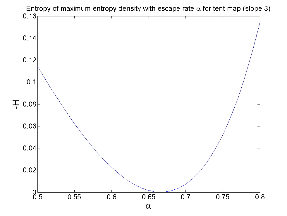
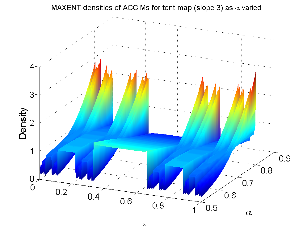
Figure 1: Example 3. Above: (neg)entropy $-H(f_{n,\alpha})$ of slope $3$ tent map ACCIMs, depending on $\alpha$ computed via MAXENT with uniform $n=1000$ subinterval partition of $[0,1]$. Below: densities of the computed ACCIMs as a function of $x\in[0,1]$ and $\alpha$.

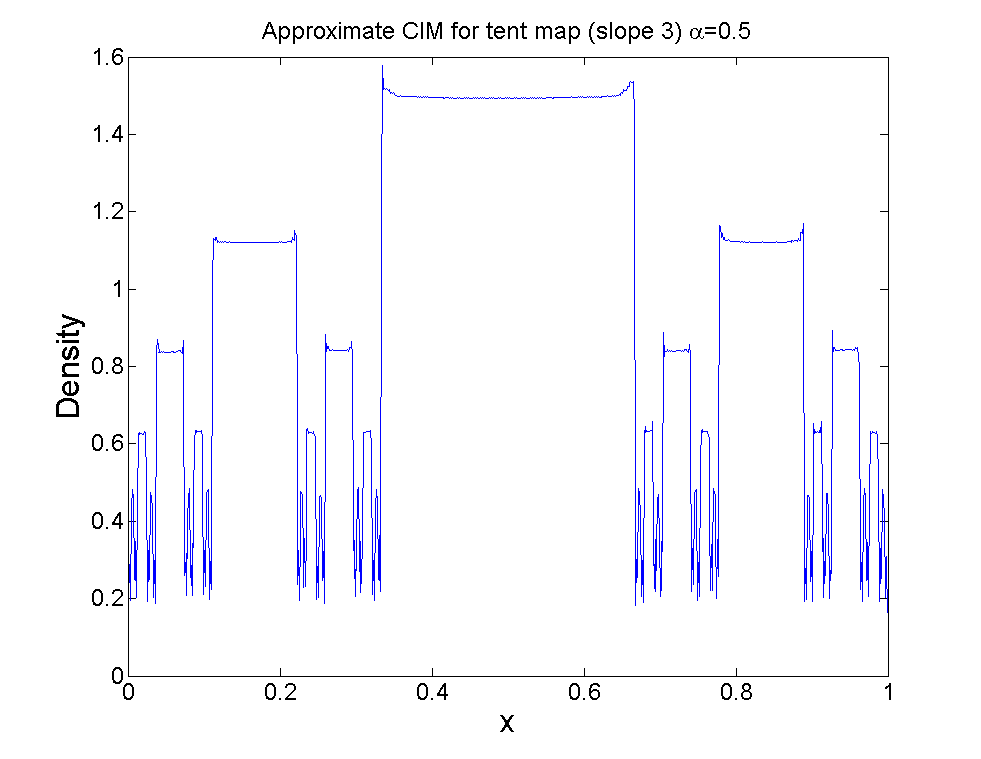
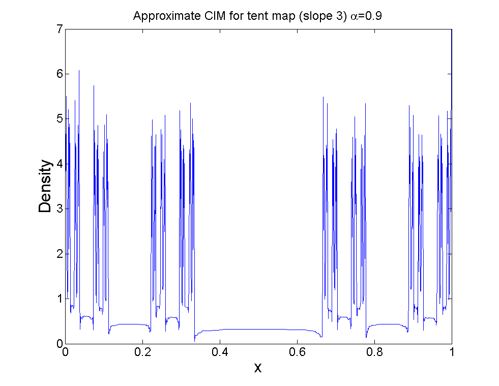
Figure 2: Example 3 (compare Figure 1). Above: approximate density $f_{1000,0.5}$ of slope $3$ tent map; note the concentration of mass on $H_{1}=[1/3,2/3]$ and its preimages. Below: approximate density $f_{1000,0.9}$ of slope $3$ tent map; note the concentration of mass on the survivor Cantor set $A_{\infty}$.

Example 4 (A linear saddle).

Let $A=[-1,1]^{2}$ and $m$ Lebesgue measure on $X=\mathbb{R}^{2}$; put $T(x,y)=(2\,x,0.8\,y)$. Then $K_{n}=[-1,1]\times\pm(0.8^{(n+1)},0.8^{n}]$, $A_{\infty}=\{0\}\times[-1,1]$ and $H_{\infty}=[-1,1]\times\{0\}\setminus(0,0)$. This linear map has a saddle-type fixed point at $(0,0)$. The only invariant measure is the delta measure at $0$. All conditionally invariant measures are supported on the local unstable manifold to the origin; in this case, the segment of the $x$–axis contained in $A$. Indeed, $m(H_{\infty})=0$ and there are no ACCIMs. There are, however, many CIMs which are AC with respect to the one-dimensional Lebesgue measure on the $x$-axis, and these are detected by the numerical method. The domain reduction to $\hat{A}$ is nontrivial here, leading to a localisation in support of the MAXENT approximations. Calculations were performed for several $\alpha$, with $10000$ test functions being the characteristic functions of a $100\times 100$ subdivision of $A$; in this case the set $\hat{A}=[-1,1]\times[-0.08,0.08]$. Some CIM estimates are presented in Figures 3 and 4.

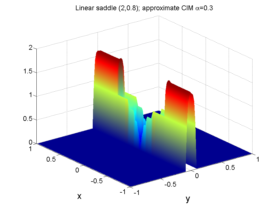
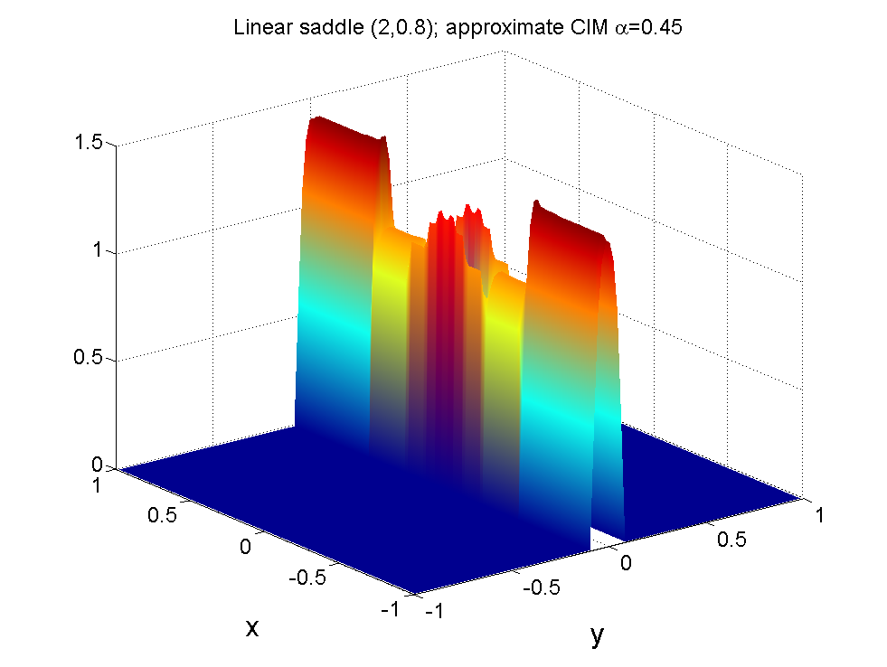
Figure 3: Example 4. MAXENT approximations of CIMs for for $\alpha=0.3$ (above) and $\alpha=0.45$ (below) for an open system with a simple saddle.

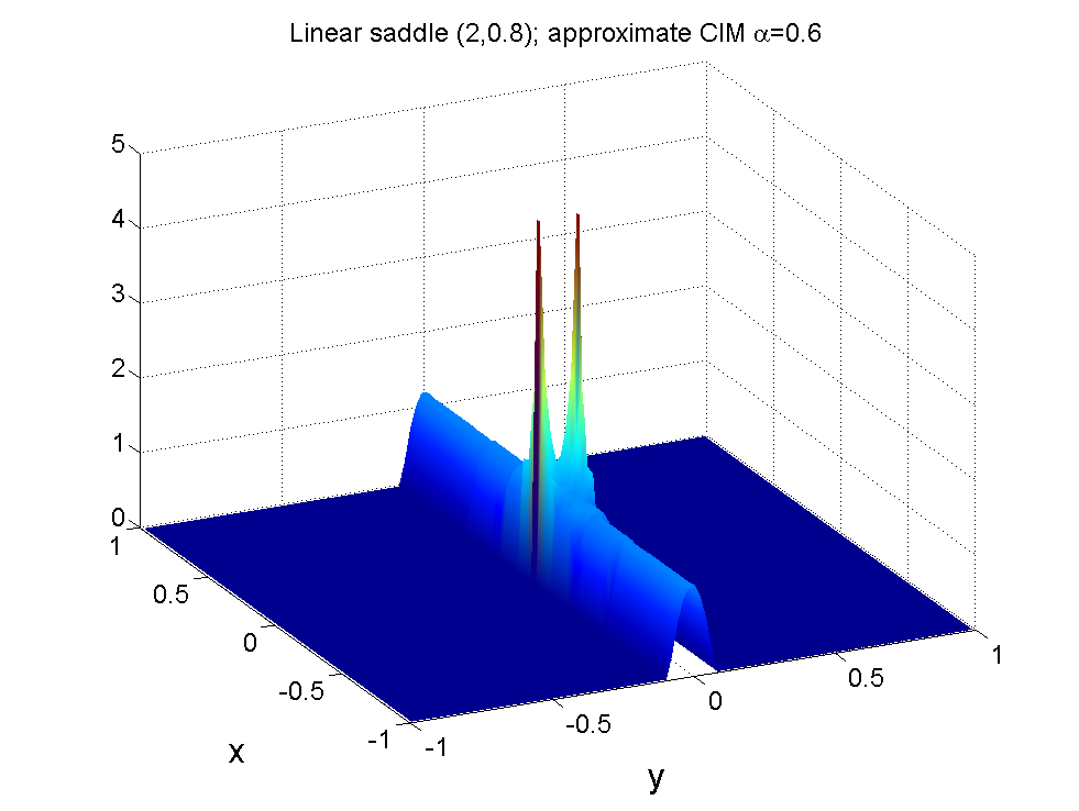
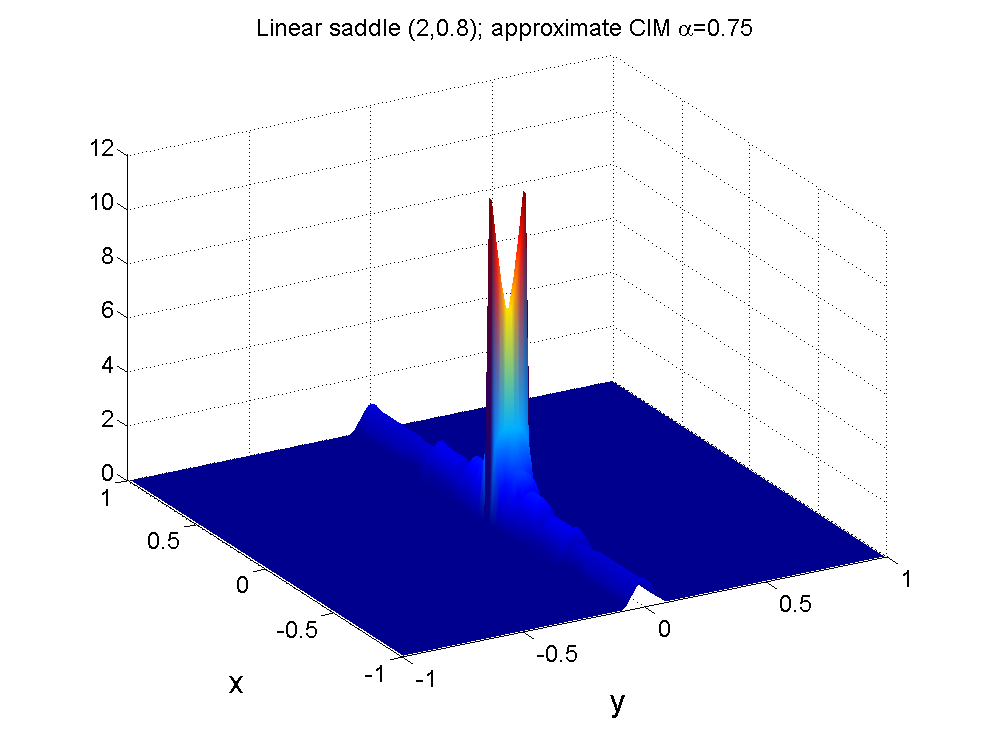
Figure 4: Example 4. MAXENT approximations of CIMs for for $\alpha=0.6$ (above) and $\alpha=0.75$ (below) for an open system with a simple saddle.

4 Concluding remarks

The MAXENT approach to calculating approximate ACCIMs has a sound analytical basis (from optimisation theory), and is easy to implement. With test functions $\{\psi_{j}\}$ derived from a partition of phase space, the basic dynamical inputs to the computational scheme are the integrals $\int\psi_{j}\circ T\,\psi_{i}\,dm$ (which could be estimated from trajectory data). For each choice of test functions, feasibility of the dual optimisation problem depends on reducing the domain of the problem to exclude certain ‘backwards transient’ parts of the phase space. With test functions derived from a partition, the resulting ‘reduced domain’ covers any recurrent set, and local unstable manifolds.

The work reported in this chapter suggests a number of avenues of future enquiry:

• are entropy-maximising ACCIMs of any particular dynamical relevance?

• given that the analysis and computation of the variational approach is similar with convex functionals other than $H(\cdot)$, are other choices of objective more appropriate?

• how is the quality of approximation affected by the choice of test functions $\{\psi_{k}\}$?

• how does the functional $H(f_{n,\alpha})$ depend on $\alpha$ (and $n$)?

• can dynamically interesting measures on unstable manifolds be recovered from this approach?

References

- [1] Afraimovich, V.S., Bunimovich, L.A.: Which hole is leaking the most: a topological approach to study open systems. Nonlinearity 23(3), 643–656 (2010). DOI 10.1088/0951-7715/23/3/012. URL http://dx.doi.org/10.1088/0951-7715/23/3/012
- [2] Bahsoun, W., Vaienti, S.: Metastability of certain intermittent maps. Nonlinearity 25(1), 107–124 (2012). DOI 10.1088/0951-7715/25/1/107. URL http://dx.doi.org/10.1088/0951-7715/25/1/107
- [3] Borwein, J., Lewis, A.: Duality relationships for entropy-like minimization problems. SIAM J. Control. Optim. 26, 325–338 (1991)
- [4] Bose, C.J., Murray, R.: Minimum ‘energy’ approximations of invariant measures for nonsingular transformations. Discrete Contin. Dyn. Syst. 14(3), 597–615 (2006)
- [5] Bose, C.J., Murray, R.: Duality and the computation of approximate invariant densities for nonsingular transformations. SIAM J. Optim. 18(2), 691–709 (electronic) (2007). DOI 10.1137/060658163. URL http://dx.doi.org/10.1137/060658163
- [6] Bruin, H., Demers, M., Melbourne, I.: Existence and convergence properties of physical measures for certain dynamical systems with holes. Ergod. Th. & Dynam. Sys. 30, 687–728 (2010)
- [7] Collett, P., Martínez, S., Schmitt, B.: The Yorke–Pianigiani measure and the asymptotic law on the limit cantor set of expanding systems. Nonlinearity 7, 1437–1443 (1994)
- [8] Collett, P., Martínez, S., Schmitt, B.: The Pianigiani–Yorke measure for topological markov chains. Israel J. Math. 97, 61–70 (1997)
- [9] Demers, M.: Markov extensions and conditionally invariant measures for certain logistic maps with small holes. Ergod. Th. & Dynam. Sys. 25, 1139–1171 (2005)
- [10] Demers, M.: Markov extensions for dynamical systems with holes: an application to expanding maps of the interval. Israel J. Math. 146, 189–221 (2005)
- [11] Demers, M.: Dispersing billiards with small holes (2013). Preprint.
- [12] Demers, M., Young, L.S.: Escape rates and conditionally invariant measures. Nonlinearity 19, 377–397 (2006). DOI 10.1088/0951-7715/19/2/008
- [13] Dolgopyat, D., Wright, P.: The diffusion coefficient for piecewise expanding maps of the interval with metastable states. Stoch. Dyn. 12(1), 1150,005, 13 (2012). DOI 10.1142/S0219493712003547. URL http://dx.doi.org/10.1142/S0219493712003547
- [14] Froyland, G.: Extracting dynamical behavior via Markov models. In: Nonlinear dynamics and statistics (Cambridge, 1998), pp. 281–321. Birkhäuser Boston, Boston, MA (2001)
- [15] Froyland, G., Dellnitz, M.: Detecting and locating near-optimal almost-invariant sets and cycles. SIAM J. Sci. Comput. 24(6), 1839–1863 (electronic) (2003). DOI 10.1137/S106482750238911X. URL http://dx.doi.org/10.1137/S106482750238911X
- [16] Froyland, G., Murray, R., Stancevic, O.: Spectral degeneracy and escape dynamics for intermittent maps with a hole. Nonlinearity 24(9), 2435–2463 (2011). DOI 10.1088/0951-7715/24/9/003. URL http://dx.doi.org/10.1088/0951-7715/24/9/003
- [17] Froyland, G., Murray, R., Terhesiu, D.: Efficient computation of topological entropy, pressure, conformal measures, and equilibrium states in one dimension. Phys. Rev. E 76(3), 036702 (2007). DOI 10.1103/PhysRevE.76.036702
- [18] González-Tokman, C., Hunt, B.R., Wright, P.: Approximating invariant densities of metastable systems. Ergodic Theory Dynam. Systems 31(5), 1345–1361 (2011). DOI 10.1017/S0143385710000337. URL http://dx.doi.org/10.1017/S0143385710000337
- [19] Homburg, A.J., Young, T.: Intermittency in families of unimodal maps. Ergodic Theory Dynam. Systems 22(1), 203–225 (2002). DOI 10.1017/S0143385702000093. URL http://dx.doi.org/10.1017/S0143385702000093
- [20] Keller, G., Liverani, C.: Rare events, escape rates and quasistationarity: some exact formulae. J. Stat. Phys. 135(3), 519–534 (2009). DOI 10.1007/s10955-009-9747-8. URL http://dx.doi.org/10.1007/s10955-009-9747-8
- [21] Liverani, C., Maume-Deschamps, V.: Lasota-Yorke maps with holes: conditionally invariant probability measures and invariant probability measures on the survivor set. Ann. Inst. H. Poincaré Probab. Statist. 39, 385–412 (2003)
- [22] Pianigiani, G., Yorke, J.: Expanding maps on sets which are almost invariant: decay and chaos. Trans. Amer. Math. Soc. 252, 351–366 (1979)
- [23] Rockafellar, R.T.: Convex analysis. Princeton University Press (1970)
- [24] Ulam, S.: A collection of mathematical problems. Interscience Publ. (1960)