Quantum and classical dissipation of charged particles

Abstract

A Hamiltonian approach is presented to study the two dimensional motion of damped electric charges in time dependent electromagnetic fields. The classical and the corresponding quantum mechanical problems are solved for particular cases using canonical transformations applied to Hamiltonians for a particle with variable mass. The Green’s function is constructed and, from it, the motion of a Gaussian wave packet is studied in detail.

1 Introduction

The motion of particles in vacuum and diverse media with dissipation has been studied in classical and quantum physics since long time. An important class of such problems are those of free electric charge carriers in a material under external time dependent electromagnetic fields. Of particular interest is the dissipation of energy through the interaction of charged carriers with the lattice ions (phonons) of the material, the carrier to carrier interaction through a Coulombian potential and, eventually, through radiation.

In classical systems damping is often described by including a velocity dependent drag term in Newton’s second law. However, the inclusion of dissipation phenomena in quantum mechanics requires special care since its building blocks, time independent Hamiltonians, lead to energy conservation. This shortcoming is remedied in the heat bath approach [1, 2] by coupling the single particle Hamiltonian with an infinite degrees of freedom system, e.g., an infinite collection of harmonic oscillators, to which the energy of the single particle is transferred. Even though the energy is conserved given that the single particle, heat bath and coupling Hamiltonians are time-independent it is difficult to handle calculations with the many degrees of freedom of the heat bath[3]. The dynamics of an open quantum system[4] is often formulated in terms of a master equation for the density matrix, that allows to work only with the single particle degrees of freedom by adding extra terms to the Von Neumann equation. Notwithstanding, the change over time of the open quantum system, in general, can not be presented in terms of a unitary time evolution[3]. Other approaches to quantum dissipation include the use of effective Schrödinger equations [5, 6] and functional integration [7, 8].

In this work, we treat the problem of energy dissipation by means of a single charged particle time dependent Hamiltonian [9, 10, 11]. In contrast to time independent Hamiltonians, in the time dependent ones the energy is no longer a conserved quantity and therefore they allow for the possibility of energy loss. In particular, we study the Hamiltonian of a charged particle with minimal coupling under a time dependent electromagnetic field with a variable mass term that accounts for energy loss. Eventhough it has been shown that the use of minimal coupling procedure to switch on electromagnetic interactions in phenomenological quantum equations of damped motion leads to incorrect equations in the classical limit[6] we show that the standard Schrödinger equation with minimal coupling and a variable mass produce correct results for the stationary state of the particles motion and allow for the modeling of the transient state by means of the time dependence of the mass.

In classical mechanics friction is usually analyzed introducing an opposing velocity-proportional force. The equation of motion of the particle can be usually built without difficulties from Newton’s second law of motion. For a one dimensional particle with mass $m$ subject to a potential $U$ one has

$$m\ddot{x}+\frac{m}{\tau}\dot{x}+\frac{\partial U}{\partial x}=0,$$ (1)

where $x$ is the position of the particle and $\tau$ is the collision time.

A deeper dynamical analysis is reached when the Hamiltonian formalism is applied. In the special case of one dimensional movement described by Eq. (1) the dynamics of a particle may be expressed by the Kanai-Caldirola (KC) Hamiltonian[9, 10, 11]

$$H=\frac{p^{2}}{2m}{\rm e}^{-t/\tau}+U\left(x\right){\rm e}^{t/\tau}.$$ (2)

This Hamiltonian even allows for analytical treatment in some simple quantum mechanical systems as a free particle[12] ($U=0$) and the harmonic oscillator[13, 14, 15, 16, 17, 18].

A great deal of effort has been focused on the modeling of dissipation phenomena for a charged particle through time dependent Hamiltonians [19, 20]. However, obtaining a Hamiltonian for a dissipative charged particle under electric and magnetic fields is not as straightforward as for the KC Hamiltonian (2). The assumption of a damping force proportional to the velocity does not lead to a Hamiltonian formulation, i.e., the Newton’s equations of motion

$$m\ddot{x}+\frac{m}{\tau}\dot{x}+qB\dot{y}-qE_{x} = 0,$$ (3)

$$m\ddot{y}+\frac{m}{\tau}\dot{y}-qB\dot{x}-qE_{y} = 0,$$ (4)

of a particle in perpendicular electric and magnetic fields $E_{x}\boldsymbol{\hat{\i}}+E_{y}\boldsymbol{\hat{\j}}$ and $B\boldsymbol{\hat{k}}$ respectively can not be obtained from a Hamiltonian approach. From here on we call this the Newtonian model.

Nevertheless, as we shall demonstrate below, it is possible to model dissipation by introducing a time-dependent mass in the Hamiltonian for a charged particle

$${H}=\frac{1}{2m\left(t\right)}\left(\boldsymbol{p}-q\boldsymbol{A}\right)^{2}+q\phi+V.$$ (5)

The aim of this work is to study the dynamics of a damped charged particle in the presence of time dependent perpendicular electric and magnetic fields by means of a time dependent Hamiltonian. We obtain the general solutions for the equations of motion for the classical, as well as for the quantum problem, via the reduction of the Hamiltonian to zero by means of a series of linear canonical transformations in the classical case and corresponding unitary transformations in the quantum mechanical one. Here it is important to stress that, in general, in a large kind of dynamical systems the number of constants of motions is not enough to reduce the Hamiltonian to zero[21]. In this work, it is assumed that the Hamiltonian is at most quadratic in the canonical coordinates, so that $\boldsymbol{A}$ is at most linear in the generalized positions, but the scalar potentials can be quadratic.

The well known classical and quantum dynamics for a constant or a variable mass charged-particle in constant perpendicular electric and magnetic fields are recovered from our analysis.

This paper is organized as follows. In Sec. 2 we review the role of time dependent masses in the Hamiltonian of charged particles interacting with electromagnetic fields. In Sec. 3 we address the solution of the classical Hamiltonian via canonical transformations. The quantum mechanical problem is introduced in Sec. 4. Unitary transformations are applied to reduce the quantum mechanical Hamiltonian in Subsec. 4.1. With the resulting time evolution unitary operator, the Green’s function is derived in Subsec. 4.2. As an example we study the dynamics of a Gaussian wave packet under the action of the Hamiltonian solved in this paper in Subsec. 4.3. We conclude in Sec. 5 with a summary of the results.

2 Hamiltonian with a variable mass.

To study the above physical problems a geometric setting is adopted. Let the kinetic energy $T$ be given by a smoothly varying family of Riemannian metrics $\langle\dot{\boldsymbol{r}},g\dot{\boldsymbol{r}}\rangle=\sum_{ij}g_{ij}(x,t)\dot{x}_{i}\dot{x}_{j}$, parametrized by time $t$ on a $n$-dimensional manifold. The Lagrangian is then

$$L=T-q\phi+q\boldsymbol{A}\cdot\dot{\boldsymbol{r}},$$ (6)

in terms of the vector potential $\boldsymbol{A}$ and the scalar potential $\phi$. The Hamiltonian is given by the Legendre transformation of the generalized velocities,

$$H = \sum_{i}p_{i}\dot{x}_{i}-L=T+q\phi-q\boldsymbol{A}\cdot\dot{\boldsymbol{r}},$$ (7)

$$p_{j} = \frac{\partial L}{\partial\dot{x}_{j}}=\sum_{k}g_{jk}\dot{x}_{k}+qA_{j},$$ (8)

and leads to a kinetic energy given in terms of the momenta as

$$T=\frac{1}{2}\left\langle\boldsymbol{p}-q\boldsymbol{A},g^{-1}\left(\boldsymbol{p}-q\boldsymbol{A}\right)\right\rangle=\frac{1}{2}\sum_{ij}(g^{-1})_{ij}\left(p_{i}-qA_{i}\right)\left(p_{j}-qA_{j}\right).$$ (9)

In this approach it is assumed then, that the media acts on the particle by means of an alteration of the metric corresponding to replace the constant mass of the particle by a time dependent effective mass. Only the flat diagonal case $g_{ij}=\delta_{ij}m(t)$, with a time dependent mass, shall be studied in here. However, more general metrics could be introduced in this manner, for example to include space inhomogeneities[22], but they shall not be considered in this work.

Let us here start with the classical Hamiltonian for a charged particle

$${H}=\frac{1}{2m}\left(\boldsymbol{p}-q\boldsymbol{A}\right)^{2}+q\phi,$$ (10)

with a time dependent mass $m$. The equations of motion obtained from (10) are

$$\dot{x}_{i}=\frac{\partial{H}}{\partial p_{i}} = \frac{p_{i}}{m}-\frac{qA_{i}}{m},$$ (11)

$$\dot{p}_{i}=-\frac{\partial{H}}{\partial x_{i}} = -\frac{q}{m}\sum_{j}\frac{\partial A_{j}}{\partial x_{i}}\left(p_{j}-qA_{j}\right)-q\frac{\partial\phi}{\partial x_{i}},$$ (12)

written as the Newton’s second law they take the following form

$$\frac{d}{dt}(m\dot{\boldsymbol{r}})=q(\boldsymbol{E}+\dot{\boldsymbol{r}}\times\boldsymbol{B}).$$ (13)

with $\boldsymbol{B}=\boldsymbol{\nabla}\times\boldsymbol{A}$ and $\boldsymbol{E}=-\boldsymbol{\nabla}\phi-\partial_{t}\boldsymbol{A}$. It must be emphasized that this equation is obtained from a Hamiltonian variational principle.

In order to illustrate how to model dissipation through a time dependent mass let us consider a charged particle in uniform perpendicular magnetic and electric fields

$$\boldsymbol{B} = B\boldsymbol{\hat{k}},$$ (14)

$$\boldsymbol{E} = E_{x}\boldsymbol{\hat{\i}}+E_{y}\boldsymbol{\hat{\j}}.$$ (15)

Separating the two components of Eq. (13) we obtain the following equations of motion for the particle

$$m\ddot{x}+\dot{m}\dot{x}+m\omega\dot{y}-qE_{x} = 0,$$ (16)

$$m\ddot{y}+\dot{m}\dot{y}-m\omega\dot{x}-qE_{y} = 0,$$ (17)

where

$$\omega=\frac{qB}{m},$$ (18)

is, in general, time dependent. Notice that for an electron ($q=-e$) for constant magnetic field and mass $\left|\omega\right|=\omega_{c}=eB/m$ is the cyclotron frequency. In stationary state ($m\ddot{x}=m\ddot{y}=0$), the solution for these equations is

$$\dot{x} = \frac{q}{\dot{m}}\frac{E_{x}+(qB/\dot{m})E_{y}}{1+(q^{2}B^{2}/\dot{m}^{2})},$$ (19)

$$\dot{y} = \frac{q}{\dot{m}}\frac{E_{y}-(qB/\dot{m})E_{x}}{1+(q^{2}B^{2}/\dot{m}^{2})}.$$ (20)

In order to test the time dependent mass model equations, specially the ones that describe the stationary state, let us try two different time dependent mass models. First we consider a KC-like mass [19, 20]

$$m=m_{0}{\rm e}^{t/\tau},$$ (21)

where, for example, $m_{0}$ and $\tau$ may be related to the effective mass and collision time in a semiconductor with mobility $\mu_{e}=nq^{2}\tau/m_{0}$ and charge carrier density $n$. Dislike the Newtonian model, in this case, the time dependent mass model yields vanishing velocity components even in the presence of an electric field. Well known results, as the magneto conductivity tensor in semiconductors [23], are contradicted by this calculation.

As a second example let us consider the following convenient choice of the mass’ time dependence

$$m=m_{0}\left(\frac{t}{\tau}+k\right),$$ (22)

where $k$ is a dimensionless positive parameter. We shall call this the linear time dependent mass model (LTDMM, for ”short”). Eq. (13) can be conveniently recast as

$$m\ddot{\boldsymbol{r}}=q(\boldsymbol{E}+\dot{\boldsymbol{r}}\times\boldsymbol{B})-\dot{m}\dot{\boldsymbol{r}}.$$ (23)

The two first terms in the right hand side of this equation correspond to the Lorentz force whereas the last term accounts for damping. Indeed, for the LTDMM

$$\dot{m}\dot{\boldsymbol{r}}=\frac{m_{0}}{\tau}\dot{\boldsymbol{r}}.$$ (24)

Here it is important to keep in mind that, despite the resemblance between Eq. (23) and the Newtonian model in Eqs. (3) and (4), in the former the mass is time dependent. Despite this difference, the stationary state for both models is the same. For the LTDMM the stationary state solution for the velocity components is in fact

$$\dot{x} = \frac{q\tau}{m_{0}}\frac{E_{x}+\omega_{0}\tau E_{y}}{1+\omega_{0}^{2}\tau^{2}},$$ (25)

$$\dot{y} = \frac{q\tau}{m_{0}}\frac{E_{y}-\omega_{0}\tau E_{x}}{1+\omega_{0}^{2}\tau^{2}}$$ (26)

where $\omega_{0}=\omega\left(t=0\right)$. Thus, our LTDMM approach and the Newtonian model given by Eqs. (3) and (4) yield the same non vanishing stationary state solution even-though their transient states might be slightly different.

However similar to the Newtonian approach, the LTDMM is only physically meaningful for $t>-k$ given that for $t\leq-k$ the mass becomes zero or even negative. One can overcome this limitation by proposing more complex models as

$$m\left(t\right)=m_{0}\ln\left(1+{\rm e}^{t/\tau}\right),$$ (27)

that yield positive non vanishing masses for all finite times and, regardless of its complexity, the same stationary state as the Newtonian and LTDMM models. Notice that this model interpolates between the KC model for $t\rightarrow-\infty$ and the LTDMM for $t\rightarrow\infty$.

To provide with a numerical example we have chosen a charged particle, e.g., an electron, in a GaAs sample with mobility $\mu_{e}=nq^{2}\tau/m_{0}=148m^{2}/Vs$, that yields a collision time $\tau=56ps$. The effective mass and charge will be set to $m_{0}=0.067m_{e}$ and $q=-e$, respectively, with $e$ the electric charge of the electron. The magnetic and electric fields are $B=40mT$ and $\boldsymbol{E}=100V/m\boldsymbol{\hat{\j}}$. The initial position and velocity of the particle are set to the origin and to $\boldsymbol{\dot{r}}=\dot{x}\left(0\right)\boldsymbol{\hat{\i}}+\dot{y}\left(0\right)\boldsymbol{\hat{\j}}=3.7Km/s\boldsymbol{\hat{\j}}$, respectively.

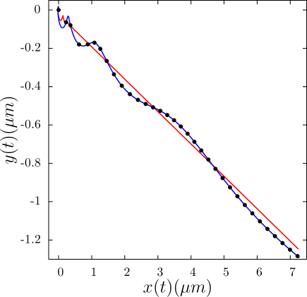
Fig. 1 shows a comparison between the parametric plots of $\boldsymbol{r}\left(t\right)=x\left(t\right)\boldsymbol{\hat{\i}}+y\left(t\right)\boldsymbol{\hat{\j}}$ for the Newtonian model (red) and the LTDMM (blue). We observe that even-though both models present different trajectories for the transient state in $t\rightarrow\infty$ they have the same overall behavior.

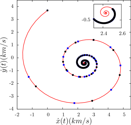
In Fig. 2 we can see a parametric plot of the velocity vector $\boldsymbol{\dot{r}}\left(t\right)=\dot{x}\left(t\right)\boldsymbol{\hat{\i}}+\dot{y}\left(t\right)\boldsymbol{\hat{\j}}$, for the LTDMM (blue dots) given by (22) and the Newtonian model (red solid line). Surprisingly both models plots are clearly over the same curve. Nevertheless we can not say that both examples behave exactly the same since the Newtonian model reaches the terminal velocity faster than the LTDMM. 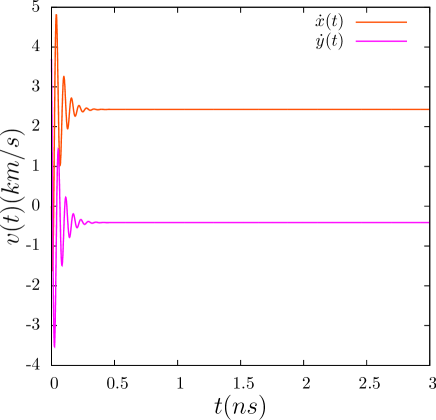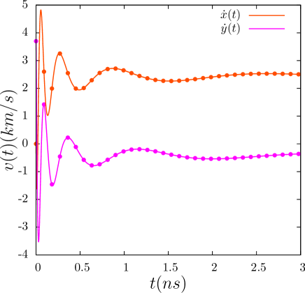This is shown in Figs. 3 and 4 where we can observe $\dot{x}$ and $\dot{y}$ plots for both models. We appreciate that the Newtonian model saturates after $t=1$ ns meanwhile the LTDMM saturates after $t=2.5$ ns.

Since the LTDMM yields similar results as the Newtonian one, and both reach the same stationary state, we shall use it through out the rest of the work for the numerical examples. Notwithstanding, all the calculations in next sections do not rely on a specific mass model.

Figure 1: (color online). Trajectory of a charged particle for the Newtonian model (red solid line) given by Eqs.(3) and (4), the linear time dependent mass model (LTDMM) defined in Eq. (22) (blue solid line) and governed by Eqs.(16) and (17) and the center of the quantum mechanical Gaussian wave packet given by Eqs. (169)-172) (black dots).

Figure 2: (color online). Parametric plot of the velocity components for a charged particle for the Newtonian model (red solid line) and the LTDMM for the classical case (blue dots) and the center of a quantum mechanical Gaussian wave packet (black points) as calculated in Subsec. 4.3.

Figure 3: (color online). Velocity components, $\dot{x}$ (blue solid line) and $\dot{y}$ (red solid line), as functions of time for the Newtonian model.

Figure 4: (color online). Velocity components, $\dot{x}$ and $\dot{y}$, as functions of time for the LTDMM and for the center of the quantum mechanical Gaussian wave packet $\dot{\zeta}_{x}^{R}$ and $\dot{\zeta}_{y}^{R}$ (points) as well.

3 The classical problem: canonical transformations

A possible procedure to solve analytically the previously depicted problem is to perform a set of canonical transformations [24]. Equivalently, also the proposal of a function of the canonical coordinates at most quadratic in the momenta, has been successful in similar problems [25]. We chose this approach for the classical problem in order to establish a connection between the canonical and the unitary quantum transformation.

The reduction of the Hamiltonian (5) is accomplished by applying canonical transformations of a certain sub-group of the affine group, namely, translations, dilatations, shears, and rotations in phase space $\xi=(x,p)^{t}$,

$$\xi\mapsto\mathbf{M}\xi+\mu,$$ (28)

with time dependent vector $\mu$, and time dependent non-singular symplectic matrix $\mathbf{M}$.

The study of a charged particle’s motion under homogeneous electric and magnetic time dependent fields, is of utmost importance in the experimental and theoretical analysis of solid state devices. The building block of any theory explaining the integer and fractional quantum Hall effects [26, 27], Shuvnikov-de Haas oscillations [28], microwave induced resistance oscillations [29], Hall induced resistance oscillations, amongst others, is the 2D electron in crossed electromagnetic fields. Therefore, we shall consider a 2D charge particle under perpendicular magnetic field

$$\boldsymbol{B}=B\boldsymbol{\hat{k}},$$ (29)

with a vector potential given by

$$\boldsymbol{A}=-\frac{B}{2}y\boldsymbol{\hat{\i}}+\frac{B}{2}x\boldsymbol{\hat{\j}}.$$ (30)

The in-plane electric field is

$$\boldsymbol{E}=\left(\frac{\dot{B}}{2}y+E_{x}\right)\boldsymbol{\hat{\i}}-\left(\frac{\dot{B}}{2}x-E_{y}\right)\boldsymbol{\hat{\j}}.$$ (31)

with a scalar potential

$$\phi=-E_{x}x-E_{y}y.$$ (32)

Here $B$, $E_{x}$ and $E_{y}$ are functions only of time.

For the sake of simplicity and without any loss of generality, we have considered the simplest gauge transformation to write down the scalar and the vector potentials.

The resulting quadratic time dependent Hamiltonian for the mentioned fields is

$$H=\frac{1}{2m}\left(p_{x}^{2}+p_{y}^{2}\right)+\frac{1}{8}\left(m\omega^{2}+\kappa\right)\left(x^{2}+y^{2}\right)\\ -\frac{\omega}{2}(xp_{y}-yp_{x})-qE_{x}x-qE_{y}y,$$ (33)

where $\omega$ is in general a time dependent parameter given by (18). In order to generalize the problem we have added a confining potential $V=\kappa\left(t\right)(x^{2}+y^{2})/8$. Since $z$ is cyclic, the momentum associated with it has been dropped but not forgotten. Here all coefficients are given smooth functions of time.

Our aim now is to reduce the Hamiltonian (33) to zero using canonical transformations (see for example [30]) of a certain sub-group of the affine group. The procedure can be summarized as follows: 1) The third term in $H$, corresponding to the coupling $z$ component of the angular momentum, can be eliminated by a rotation leaving the first two terms invariant. The result is a Hamiltonian for two uncoupled one dimensional harmonic oscillators with variable masses and frequencies, as those considered in the literature; 2) a time dependent translation is performed to eliminate the linear contributions leading to an harmonic oscillator Hamiltonian with time dependent coefficients; 3) and, finally a dilatation and two shears are applied to reduce the Hamiltonian to zero; hence, the final generalized momenta and positions are simultaneously constants of the motion and the original initial conditions, $(p_{0},q_{0})$, of our problem.

For the first step in our program we require the generating function of a rotation $R$ for a finite angle $\theta(t)$ given by

$$F_{1}=q^{t}R^{t}p_{1}=xp_{x_{1}}\cos\theta+yp_{x_{1}}\sin\theta-xp_{y_{1}}\sin\theta+yp_{y_{1}}\cos\theta,$$ (34)

with the column vectors $q=(x,y)^{t}$ and $p_{1}=(p_{x_{1}},p_{y_{1}})^{t}$, being $p_{1}=Rp$ and $q_{1}=Rq$ the rotated coordinates. By means of this generating function we obtain the following transformation rules

$$x_{1} = \frac{\partial F_{1}}{\partial p_{x_{1}}}=x\cos\theta+y\sin\theta,$$ (35)

$$y_{1} = \frac{\partial F_{1}}{\partial p_{y_{1}}}=-x\sin\theta+y\cos\theta,$$ (36)

and

$$p_{x} = \frac{\partial F_{1}}{\partial x}=p_{x_{1}}\cos\theta-p_{y_{1}}\sin\theta,$$ (37)

$$p_{y} = \frac{\partial F_{1}}{\partial y}=p_{x_{1}}\sin\theta+p_{y_{1}}\cos\theta.$$ (38)

Notice that we directly obtain the canonical transformations for $p_{x_{1}}$ and $p_{y_{1}}$, given by the previous expressions, (37) and (38), but we need to solve equations (35) and (36) to obtain the corresponding ones for $x$ and $y$

$$x = {x_{1}}\cos\theta-y_{1}\sin\theta,$$ (39)

$$y = x_{1}\sin\theta+y_{1}\cos\theta.$$ (40)

Hence, the first transformed Hamiltonian is

$$H_{1}={H}^{R}+\frac{\partial F_{1}}{\partial t}=\frac{1}{2m}\left(p_{x_{1}}^{2}+p_{y_{1}}^{2}\right)-\left(\frac{\omega}{2}+\dot{\theta}\right)\left(y_{1}p_{x_{1}}-x_{1}p_{y_{2}}\right)\\ +\frac{1}{8}\left(m\omega^{2}+\kappa\right)\left(x_{1}^{2}+y_{1}^{2}\right)-qE_{x}^{R}x_{1}-qE_{y}^{R}y_{1}.$$ (41)

Here ${H}^{R}$ is the original function, but now expressed in terms of the transformed coordinates and the rotated electric field

$$E_{x}^{R} = E_{x}\cos\theta+E_{y}\sin\theta,$$ (42)

$$E_{y}^{R} = -E_{x}\sin\theta+E_{y}\cos\theta.$$ (43)

In order to reduce the angular momentum term in Eq. (41), we set

$$\dot{\theta}=-\frac{\omega}{2},$$ (44)

and we obtain the direct sum of two one dimensional harmonic oscillator-like Hamiltonians

$${H}_{1}=\frac{1}{2m}\left(p_{x_{1}}^{2}+p_{y_{1}}^{2}\right)+\frac{1}{8}\left(m\omega^{2}+\kappa\right)\left(x_{1}^{2}+y_{1}^{2}\right)-qE_{x}^{R}x_{1}-qE_{y}^{R}y_{1}.$$ (45)

All linear terms can now be reduced via space and momentum translations with the generating function

$$F_{2}=\left(x_{1}-\lambda_{x}\right)\left(p_{x_{2}}-\pi_{x}\right)+\left(y_{1}-\lambda_{y}\right)\left(p_{y_{2}}-\pi_{y}\right)-S,$$ (46)

that yields the following transformation rules

$$x_{2} = \frac{\partial F_{2}}{\partial p_{x_{2}}}=x_{1}-\lambda_{x},$$ (47)

$$y_{2} = \frac{\partial F_{2}}{\partial p_{y_{2}}}=y_{1}-\lambda_{y},$$ (48)

$$p_{x_{1}} = \frac{\partial F_{2}}{\partial x_{1}}=p_{x_{2}}-\pi_{x},$$ (49)

$$p_{y_{1}} = \frac{\partial F_{2}}{\partial y_{1}}=p_{y_{2}}-\pi_{y},$$ (50)

where $x_{2}$, $y_{2}$, $p_{x_{2}}$ and $p_{y_{2}}$ are the new variables and $S$ is the action. Here, $\lambda_{x}$ and $\lambda_{y}$ are time dependent parameters for the translation in coordinates, meanwhile $\pi_{x}$ and $\pi_{y}$ are the corresponding ones for the momentum space. In order to obtain the canonical transformations for $x_{1}$ and $y_{1}$, we solve (47) and (48)

$$x_{1} = x_{2}+\lambda_{x},$$ (51)

$$y_{1} = y_{2}+\lambda_{y}.$$ (52)

After transforming via $F_{2}$ the resulting Hamiltonian is

$$H_{2}=\frac{1}{2m}\left(p_{x_{2}}^{2}+p_{y_{2}}^{2}\right)+\frac{1}{8}\left(m\omega^{2}+\kappa\right)\left(x_{2}^{2}+y_{2}^{2}\right)\\ -\left(\frac{\pi_{x}}{m}+\dot{\lambda}_{x}\right)p_{x_{2}}-\left(\frac{\pi_{y}}{m}+\dot{\lambda}_{y}\right)p_{y_{2}}\\ +\left[\frac{1}{4}\left(m\omega^{2}+\kappa\right)\lambda_{x}-qE_{x}^{R}-\dot{\pi}_{x}\right]x_{2}+\left[\frac{1}{4}\left(m\omega^{2}+\kappa\right)\lambda_{y}-qE_{y}^{R}-\dot{\pi}_{y}\right]y_{2}\\ +\frac{1}{2m}\left(\pi_{x}^{2}+\pi_{y}^{2}\right)+\frac{1}{8}\left(m\omega^{2}+\kappa\right)\left(\lambda_{x}^{2}+\lambda_{y}^{2}\right)\\ -qE_{x}^{R}\lambda_{x}-qE_{y}^{R}\lambda_{y}+\dot{\lambda}_{x}\pi_{x}+\dot{\lambda}_{y}\pi_{y}-\dot{S}.$$ (53)

In Hamiltonian $H_{2}$ the coefficients of $x_{2}$, $y_{2}$, $p_{x2}$ and $p_{y2}$ correspond to the Euler equations of the classical Lagrangian

$$L_{1}=\frac{1}{2m}\left(\pi_{x}^{2}+\pi_{y}^{2}\right)+\frac{1}{8}\left(m\omega^{2}+\kappa\right)\left(\lambda_{x}^{2}+\lambda_{y}^{2}\right)\\ -qE_{x}^{R}\lambda_{x}-qE_{y}^{R}\lambda_{y}+\dot{\lambda}_{x}\pi_{x}+\dot{\lambda}_{y}\pi_{y}$$ (54)

for the translation parameters $\lambda_{x}$,$\lambda_{y}$, $\pi_{x}$ and $\pi_{y}$. In order for all the linear coefficients to vanish we require that this Lagrangian be the solution of the Euler equations for the translation parameters:

$$\frac{d}{dt}\frac{\partial L_{1}}{\partial\dot{\pi}_{x}}-\frac{\partial L_{1}}{\partial\pi_{x}} = -\left(\frac{\pi_{x}}{m}+\dot{\lambda}_{x}\right)=0,$$ (55)

$$\frac{d}{dt}\frac{\partial L_{1}}{\partial\dot{\pi}_{y}}-\frac{\partial L_{1}}{\partial\pi_{y}} = -\left(\frac{\pi_{y}}{m}+\dot{\lambda}_{y}\right)=0,$$ (56)

$$\frac{d}{dt}\frac{\partial L_{1}}{\partial\dot{\lambda}_{x}}-\frac{\partial L_{1}}{\partial\lambda_{x}} = \frac{m\omega^{2}+\kappa}{4}\lambda_{x}-qE_{x}^{R}-\dot{\pi}_{x}=0,$$ (57)

$$\frac{d}{dt}\frac{\partial L_{1}}{\partial\dot{\lambda}_{y}}-\frac{\partial L_{1}}{\partial\lambda_{y}} = \frac{m\omega^{2}+\kappa}{4}\lambda_{y}-qE_{y}^{R}-\dot{\pi}_{y}=0.$$ (58)

Additionally, to remove the Lagrangian part, $L_{1}-\dot{S}=0$ must be fulfilled and consequently $\dot{S}$ can be associated with the time derivative of the corresponding action.

The transformed Hamiltonian $H_{2}$ is thus simplified into

$$H_{2}=\frac{1}{2m}\left(p_{x_{2}}^{2}+p_{y_{2}}^{2}\right)+\frac{1}{8}\left(m\omega^{2}+\kappa\right)\left(x_{2}^{2}+y_{2}^{2}\right).$$ (59)

The harmonic oscillator coefficient $m\omega^{2}+\kappa$ can be expressed in terms of new parameters as

$$m\omega^{2}+\kappa=m_{0}\omega_{0}^{2}{\rm e}^{2\beta-\alpha},$$ (60)

where ${\rm e}^{2\beta}=f^{2}(t)+\kappa_{0}e^{\alpha}g(t)/m_{0}\omega_{0}^{2}$ contains the explicit time dependence of the given magnetic field $B=B_{0}f(t)$, the confining potential $\kappa=\kappa_{0}g(t)$ and

$$m\left(t\right)=m_{0}{\rm e}^{\alpha\left(t\right)}.$$ (61)

In terms of this variables, the Hamiltonian is rewritten as [31]

$$H_{2}=\frac{e^{-\alpha}}{2m_{0}}\left(p_{x_{2}}^{2}+p_{y_{2}}^{2}\right)+\frac{1}{8}m_{0}\omega_{0}^{2}e^{2\beta-\alpha}\left(x_{2}^{2}+y_{2}^{2}\right).$$ (62)

As a next step we consider a dilatation and two shears. The generating function for such a transformation is

$$F_{3}=\frac{e^{\frac{1}{2}\gamma}}{\cos\delta}\left(x_{2}p_{x_{3}}+y_{2}p_{y_{3}}\right)-\frac{e^{\gamma}\tan\delta}{2\Delta}\left(p_{x_{3}}^{2}+p_{y_{3}}^{2}\right)-\frac{\Delta\tan\delta}{2}\left(x_{2}^{2}+y_{2}^{2}\right)$$ (63)

with time dependent functions $\gamma$, $\delta$ and $\Delta$. $F_{3}$ produces the following transformation rules

$$x_{3} = \frac{\partial F_{3}}{\partial p_{x_{3}}}=\frac{e^{\frac{1}{2}\gamma}}{\cos\delta}x_{2}-\frac{e^{\gamma}\tan\delta}{\Delta}p_{x_{3}},$$ (64)

$$y_{3} = \frac{\partial F_{3}}{\partial p_{y_{3}}}=\frac{e^{\frac{1}{2}\gamma}}{\cos\delta}y_{2}-\frac{e^{\gamma}\tan\delta}{\Delta}p_{y_{3}},$$ (65)

$$p_{x_{2}} = \frac{\partial F_{3}}{\partial x_{2}}=\frac{e^{\frac{1}{2}\gamma}}{\cos\delta}p_{x_{3}}-\Delta\tan\delta\ x_{2},$$ (66)

$$p_{y_{2}} = \frac{\partial F_{3}}{\partial y_{2}}=\frac{e^{\frac{1}{2}\gamma}}{\cos\delta}p_{y_{3}}-\Delta\tan\delta\ y_{2}.$$ (67)

We can obtain the corresponding canonical transformations by solving $x_{2}$, $y_{2}$, $p_{x_{2}}$ and $p_{y_{2}}$ from the previous equations

$$x_{2} = e^{-\frac{1}{2}\gamma}x_{3}\cos\delta+\frac{e^{\frac{1}{2}\gamma}}{\Delta}p_{x_{3}}\sin\delta$$ (68)

$$p_{x_{2}} = e^{\frac{1}{2}\gamma}p_{x_{3}}\cos\delta-e^{-\frac{1}{2}\gamma}\Delta\ x_{3}\sin\delta$$ (69)

$$y_{2} = e^{-\frac{1}{2}\gamma}y_{3}\cos\delta+\frac{e^{\frac{1}{2}\gamma}}{\Delta}p_{y_{3}}\sin\delta$$ (70)

$$p_{y_{2}} = e^{\frac{1}{2}\gamma}p_{y_{3}}\cos\delta-e^{-\frac{1}{2}\gamma}\Delta\ y_{3}\sin\delta.$$ (71)

Notice that even though the generating function $F_{3}$ in Eq. (63) and (64)-(67) have multiple divergences when $\delta=(2n-1)\pi/2$, its corresponding canonical transformation rules (68)-(71) have non. These are the well known Arnold transformations[32, 33]. It is possible to show that they comply with condition necessary to preserve the value of the Wronskian

$$\det\left(\begin{array}[]{cc}{\rm e}^{-\frac{1}{2}\gamma}\cos\delta&\frac{e^{\frac{1}{2}\gamma}}{\Delta}\sin\delta\\ -{\rm e}^{-\frac{1}{2}\gamma}\Delta\sin\delta&e^{\frac{1}{2}\gamma}\cos\delta\end{array}\right)=1$$ (72)

and for the transformation matrix to be symplectic.

Under $F_{3}$, the new transformed Hamiltonian is

$$H_{3}=\left[e^{-\alpha}\left(\frac{\Delta}{m_{0}}\cos^{2}\delta+\frac{m_{0}\omega_{0}^{2}e^{2\beta}}{4\Delta}\sin^{2}\delta\right)-\dot{\delta}+\sin\delta\cos\delta\frac{\dot{\Delta}}{\Delta}\right]\frac{e^{\gamma}}{2\Delta}\left(p_{x_{3}}^{2}+p_{y_{3}}^{2}\right)\\ +\left[e^{-\alpha}\left(\frac{\Delta}{m_{0}}\sin^{2}\delta+\frac{m_{0}\omega_{0}^{2}e^{2\beta}}{4\Delta}\cos^{2}\delta\right)-\dot{\delta}-\sin\delta\cos\delta\frac{\dot{\Delta}}{\Delta}\right]\frac{\Delta e^{-\gamma}}{2}\left(x_{3}^{2}+y_{3}^{2}\right)\\ +\left[e^{-\alpha}\left(-\frac{\Delta}{m_{0}}+\frac{m_{0}\omega_{0}^{2}e^{2\beta}}{4\Delta}\right)\sin\delta\cos\delta+\frac{\dot{\gamma}}{2}-\sin^{2}\delta\frac{\dot{\Delta}}{\Delta}\right]\left(x_{3}p_{x_{3}}+y_{3}p_{y_{3}}\right).$$ (73)

In order to obtain a null Hamiltonian we set the coefficients of $\left(p_{x_{3}}^{2}+p_{y_{3}}^{2}\right)$, $\left(x_{3}^{2}+y_{3}^{2}\right)$ and $\left(x_{3}p_{x_{3}}+y_{3}p_{y_{3}}\right)$ to zero. We, thus, obtain the following system of coupled differential equations for the transformation parameters

$$0 = e^{-\alpha}\left(\frac{\Delta}{m_{0}}\cos^{2}\delta+\frac{m_{0}\omega_{0}^{2}e^{2\beta}}{4\Delta}\sin^{2}\delta\right)-\dot{\delta}+\sin\delta\cos\delta\frac{\dot{\Delta}}{\Delta},$$ (74)

$$0 = e^{-\alpha}\left(\frac{\Delta}{m_{0}}\sin^{2}\delta+\frac{m_{0}\omega_{0}^{2}e^{2\beta}}{4\Delta}\cos^{2}\delta\right)-\dot{\delta}-\sin\delta\cos\delta\frac{\dot{\Delta}}{\Delta},$$ (75)

$$0 = e^{-\alpha}\left(-\frac{\Delta}{m_{0}}+\frac{m_{0}\omega_{0}^{2}e^{2\beta}}{4\Delta}\right)\sin\delta\cos\delta+\frac{\dot{\gamma}}{2}-\sin^{2}\delta\frac{\dot{\Delta}}{\Delta}.$$ (76)

The solutions to this differential equations cancel the whole Hamiltonian $H_{3}$. In such a case $x_{3}$, $y_{3}$, $p_{x_{3}}$ and $p_{y_{3}}$ are constant in time and, therefore, they are constants of the motion. To simplify the structure of the differential equations and their solutions we propose

$$\Delta=\frac{1}{2}m_{0}\omega_{0}e^{\beta+\eta},$$ (77)

where $\eta$ is a time dependent function, yielding a simplification of the previous coupled equations

$$\dot{\delta} = \frac{1}{2}\omega_{0}e^{\beta-\alpha}\cosh\eta,$$ (78)

$$\dot{\eta}+\dot{\beta} = \frac{1}{2}\omega_{0}e^{\beta-\alpha}\sinh\eta\left(\tan\delta-\cot\delta\right),$$ (79)

$$\dot{\gamma} = \omega_{0}e^{\beta-\alpha}\sinh\eta\tan\delta.$$ (80)

For practical purposes the solutions of these equations, in the most general case, can be obtained by numerical methods. Nevertheless, it is possible to extract information from (78)-(80) by grouping the last three equations in a single hyperbolic one

$$\frac{\dot{\delta}^{2}}{a^{2}}-\frac{\left(\dot{\gamma}-\dot{\beta}-\dot{\eta}\right)^{2}}{b^{2}}=1,$$ (81)

here $a=\omega_{0}e^{\beta-\alpha}/2$ and $b=\omega_{0}e^{\beta-\alpha}/\sin 2\delta$. If we use the $\eta$ function as a parameter, we can rewrite the hyperbola with the parametric functions (78) and

$$\dot{\gamma}-\dot{\beta}-\dot{\eta}=\frac{\omega_{0}e^{\beta-\alpha}}{\sin 2\delta}\sinh\eta.$$ (82)

For a given problem with no parabolic potential, $\kappa_{0}=0$, only one of the branches contains the physical solution. Each branch is associated with a given rotating direction of the charged particle.

In particular, the vertices of the hyperbola correspond to the constant magnetic field case. If we set ourselves in one of the vertices $\dot{\delta}=\omega_{0}e^{\beta-\alpha}/2$ and by comparing with (78) we obtain that $\eta=0$ and, consequently, $\dot{\beta}=0$ and $\dot{\gamma}=0$. This is indeed the case when the magnetic field is a constant, i. e. $\beta=0$ and $\gamma=0$. In this manner we find that with an appropriate time dependent mass model and the initial condition $\delta(0)=0$ we can integrate $\dot{\delta}=\omega_{0}e^{-\alpha}/2$ and obtain $\delta$, the only relevant parameter under the conditions described above.

It is well-known that the time reversal symmetry is broken by a constant magnetic field, even though we have a frictionless problem, this symmetry breaking is the cause of the existence two vertices. More generally, for a problem where the magnetic field is a function of time, the solution is given by another region at the hyperbola branch. In other words, the hyperbolic behavior of Eqs. (78)-(80) is a consequence of the magnetic field’s time reversal asymmetry.

The last transformation gives the solution to the initial problem describing the motion of a charged particle under the influence of the potentials (32) and (30) where the electric and magnetic fields are only time-dependent functions. Under the previous three transformations, we find that $x_{3}$, $y_{3}$, $p_{x_{3}}$ and $p_{y_{3}}$ are constants along the classical orbit followed by the particle. In other words, $x_{3}$, $y_{3}$, $p_{x_{3}}$ and $p_{y_{3}}$ are the initial conditions and we shall rename them as $x_{3}=x_{0}$, $y_{3}=y_{0}$, $p_{x_{3}}=p_{x_{0}}$ and $p_{y_{3}}=p_{y_{0}}$.

It is also possible to figure out a single canonical transformation after adequately collecting all the above contributions into the following form

$$\xi={\bf M}\xi_{0}+\mu,$$ (83)

where ${\bf M}$ is a symplectic matrix given by

$${\bf M}=\left[\begin{array}[]{cc}{\bf a}&{\bf b}\\ {\bf c}&{\bf d}\end{array}\right]=\left[\begin{array}[]{cc}e^{-\frac{\gamma}{2}}\cos\theta\cos\delta&-e^{-\frac{\gamma}{2}}\sin\theta\cos\delta\\ \frac{e^{\frac{\gamma}{2}}}{\Delta}\sin\theta\sin\delta&\frac{e^{\frac{\gamma}{2}}}{\Delta}\cos\theta\sin\delta\\ e^{\frac{\gamma}{2}}\cos\theta\cos\delta&-e^{\frac{\gamma}{2}}\sin\theta\cos\delta\\ e^{\frac{\gamma}{2}}\sin\theta\cos\delta&e^{\frac{\gamma}{2}}\cos\theta\cos\delta\\ \end{array}\right.\\ \left.\begin{array}[]{cc}\frac{e^{\frac{\gamma}{2}}}{\Delta}\cos\theta\sin\delta&-\frac{e^{\frac{\gamma}{2}}}{\Delta}\sin\theta\sin\delta\\ \frac{e^{\frac{\gamma}{2}}}{\Delta}\sin\theta\sin\delta&\frac{e^{\frac{\gamma}{2}}}{\Delta}\cos\theta\sin\delta\\ e^{\frac{\gamma}{2}}\cos\theta\cos\delta&-e^{\frac{\gamma}{2}}\sin\theta\cos\delta\\ e^{\frac{\gamma}{2}}\sin\theta\cos\delta&e^{\frac{\gamma}{2}}\cos\theta\cos\delta\\ \end{array}\right]$$ (84)

and

$$\mu=\left[\begin{array}[]{cccc}\cos\theta&-\sin\theta&0&0\\ \sin\theta&\cos\theta&0&0\\ 0&0&\cos\theta&-\sin\theta\\ 0&0&\sin\theta&\cos\theta\\ \end{array}\right]\left[\begin{array}[]{c}\lambda_{x}\\ \lambda_{y}\\ -\pi_{x}\\ -\pi_{y}\end{array}\right].$$ (85)

As an example, we consider the simplest case when the magnetic field and the mass are constants, meanwhile both the confining potential and the electric field are absent. In such a case $\delta=-\theta=\omega_{0}/2t$, $\Delta=m_{0}\omega_{0}/2$ and there is no dilatation, hence $\gamma=0$ and $\eta=0$. By using equation (83) all the position and the momentum variables can be expressed as a function of time and the initial conditions

$$\left[\begin{array}[]{c}x\\ y\\ p_{x}\\ p_{y}\end{array}\right]=\left[\begin{array}[]{cc}\frac{1}{2}\left(1+\cos\omega_{0}t\right)&\frac{1}{2}\sin\omega_{0}t\\ -\frac{1}{2}\sin\omega_{0}t&\frac{1}{2}\left(1+\cos\omega_{0}t\right)\\ -\frac{1}{4}m_{0}\omega_{0}\sin\omega_{0}t&\frac{1}{4}m_{0}\omega_{0}\left(\cos\omega_{0}t-1\right)\\ \frac{1}{4}m_{0}\omega_{0}\left(1-\cos\omega_{0}t\right)&-\frac{1}{4}m_{0}\omega_{0}\sin\omega_{0}t\end{array}\right.\\ \left.\begin{array}[]{cc}\frac{\sin\omega_{0}t}{m_{0}\omega_{0}}&\frac{1-\cos\omega_{0}t}{m_{0}\omega_{0}}\\ \frac{\cos\omega_{0}t-1}{m_{0}\omega_{0}}&\frac{\sin\omega_{0}t}{m_{0}\omega_{0}}\\ \frac{1}{2}\left(1+\cos\omega_{0}t\right)&\frac{1}{2}\sin\omega_{0}t\\ -\frac{1}{2}\sin\omega_{0}t&\frac{1}{2}\left(1+\cos\omega_{0}t\right)\end{array}\right]\left[\begin{array}[]{c}x_{0}\\ y_{0}\\ p_{x_{0}}\\ p_{y_{0}}\end{array}\right].$$ (86)

This last result is consistent with the solution obtained directly from the Hamilton equations of motion. The motion described in the previous equations is periodic, with period $T=2\pi/\omega_{0}$ and $\omega_{0}$ is the Larmor frequency. The periodicity can be deduced from the behavior of the block matrices ${\bf a}$ and ${\bf d}$ in (84) since they become unit matrices for $t=T$, meanwhile ${\bf b}$ and ${\bf c}$ become zero. The charged particle is moving around a circular orbit in the plane $xy$ with radius $r=\sqrt{p_{x_{0}}^{2}+p_{y_{0}}^{2}}/m_{0}\omega_{0}$. Physically, the trajectories of the particles are curved due to the Lorentz force, nevertheless, when the magnetic field $B_{0}$ is small, the motion of the particles is almost linear ($r$ grows). For larger values of $B_{0}$, the particle’s motion is highly curved ($r$ decreases). The last feature is given by the off-diagonal block matrices ${\bf b}$ and ${\bf c}$.

It is important to notice that in the Hamiltonian $H_{3}$ we can set the two first coefficients to $\omega_{0}/2$ instead of zero as in Eqs.(74) and (75), meanwhile we keep the null equation (76). In this case we obtain a KC-like Hamiltonian, but the equations that must be satisfied in order to obtain a solution are much more complex.

4 The quantum problem: unitary transformations

The classical calculations presented in the previous section allow to set a framework for a quantum mechanical analog of (33) through the Schrödinger’s equation

$$\hat{H}\left|\psi\left(t\right)\right\rangle=\hat{p}_{t}\left|\psi\left(t\right)\right\rangle,$$ (87)

where, the quantum mechanical Hamiltonian is given by

$$\hat{H}=\frac{1}{2m}\left(\boldsymbol{\hat{p}}-q\boldsymbol{\hat{A}}\right)^{2}+q\phi+\frac{\kappa}{8}\left(\hat{x}^{2}+\hat{y}^{2}\right).$$ (88)

Here, $\hat{p}_{t}$ is the energy operator, i.e., $\hat{p}_{t}\rightarrow i\hbar\partial_{t}$ and $\hat{x}$, $\hat{y}$, $\hat{p}_{x}$ and $\hat{p}_{y}$ are the space and momentum operators such that

$$\hat{x}\left|x,y\right\rangle = x\left|x,y\right\rangle,$$ (89)

$$\hat{y}\left|x,y\right\rangle = y\left|x,y\right\rangle,$$ (90)

$$\hat{p}_{x}\left|p_{x},p_{y}\right\rangle = p_{x}\left|p_{x},p_{y}\right\rangle,$$ (91)

$$\hat{p}_{y}\left|p_{x},p_{y}\right\rangle = p_{x}\left|p_{x},p_{y}\right\rangle,$$ (92)

where $\left|x,y\right\rangle$ and $\left|p_{x},p_{y}\right\rangle$ are the space and momentum eigenstates respectively. The space and momentum operators follow the usual commutation relations

$$\left[\hat{x}_{i},\hat{p}_{j}\right]=i\hbar\delta_{i,j},$$ (93)

as well as the energy operator and time

$$\left[\hat{p}_{t},t\right]=i\hbar.$$ (94)

The physical electric and magnetic fields $\boldsymbol{E}$ and $\boldsymbol{B}$, respectively, are obtained as usual from the scalar and vector potentials $\phi$ and $\boldsymbol{A}$ by the relations (29) and (31) as we discussed in Sec. 2.

The integration of the quantum mechanical problem follows the same path as the classical problem. The reduction of the Hamiltonian is now easily achieved by unitary transformations [34, 35, 36, 37], each one associated to one of the three classical canonical transformations applied in Sec. 3. Each reduction step has the following structure

$$U\hat{H}U^{{\dagger}}U\left|\psi\left(t\right)\right\rangle=U\hat{p}_{t}U^{{\dagger}}U\left|\psi\left(t\right)\right\rangle\Rightarrow\hat{H}^{\prime}\left|\psi^{\prime}\left(t\right)\right\rangle=\hat{p}_{t}\left|\psi^{\prime}\left(t\right)\right\rangle$$ (95)

with $\hat{H}^{\prime}=U\hat{H}U^{{\dagger}}-U\left[\hat{p}_{t},U^{{\dagger}}\right]$, and $\left|\psi^{\prime}\left(t\right)\right\rangle=U\left|\psi\left(t\right)\right\rangle$.

The Floquet operator is thus given by

$$\hat{\mathcal{H}}=\hat{H}-\hat{p}_{t},$$ (96)

and the Schrödinger’s equation takes the compact form

$$\hat{\mathcal{H}}\left|\psi\left(t\right)\right\rangle=\left(\hat{H}-\hat{p}_{t}\right)\left|\psi\left(t\right)\right\rangle=0.$$ (97)

Our aim now is to study the Hamiltonian in Eq. (88) for the particular case analyzed in Sec. 3 of a magnetic and a perpendicular electric fields of Eqs. (29) and (31). Such fields can be obtained from the potentials in (30) and (32). The quantum mechanical potentials are thus given by

$$\boldsymbol{A} = \frac{B}{2}\left(-\hat{y}\boldsymbol{\hat{\i}}+\hat{x}\boldsymbol{\hat{\j}}\right),$$ (98)

$$\phi = -E_{x}\left(t\right)\hat{x}-E_{y}\left(t\right)\hat{y}.$$ (99)

In this gauge, the Floquet operator takes the following form

$$\hat{\mathcal{H}}=\frac{1}{2m}\left[\left(\hat{p}_{x}+\frac{qB}{2}\hat{y}\right)^{2}+\left(\hat{p}_{y}-\frac{qB}{2}\hat{x}\right)^{2}\right]\\ -q\left[E_{x}\left(t\right)\hat{x}+E_{y}\left(t\right)\hat{y}\right]+\frac{\kappa}{8}\left(\hat{x}^{2}+\hat{y}^{2}\right)-\hat{p}_{t}.$$ (100)

4.1 Evolution operator

To obtain the evolution operator for the Hamiltonian in (88) in the presence of the magnetic and electric fields given by Eqs. (29) and (31), respectively, we proceed in a similar fashion to the classical case in Sec. 3. We apply a series of unitary transformations, each corresponding to a canonical transformation of the classical case.

The first unitary transformation, a rotation around the $z$ axis [34], corresponds to the canonical transformation in Eq. (34) and is given by

$$U_{1}=\exp\left(i\frac{\theta\hat{L}_{z}}{\hbar}\right),$$ (101)

where $\hat{L}_{z}=\hat{x}\hat{p}_{y}-\hat{y}\hat{p}_{x}$ is the angular momentum along the $z$ axis. It has the following effect on the position, momentum and energy operators

$$U_{1}\hat{x}U_{1}^{{\dagger}} = \hat{x}\cos\theta-\hat{y}\sin\theta,$$ (102)

$$U_{1}\hat{y}U_{1}^{{\dagger}} = \hat{x}\sin\theta+\hat{y}\cos\theta,$$ (103)

$$U_{1}\hat{p}_{x}U_{1}^{{\dagger}} = \hat{p}_{x}\cos\theta-\hat{p}_{y}\sin\theta,$$ (104)

$$U_{1}\hat{p}_{y}U_{1}^{{\dagger}} = \hat{p}_{x}\sin\theta+\hat{p}_{y}\cos\theta,$$ (105)

$$U_{1}\hat{p}_{t}U_{1}^{{\dagger}} = \hat{p}_{t}+\dot{\theta}\hat{L}_{z}.$$ (106)

Note that $U_{1}$ leaves invariant the quadratic forms $\hat{x}^{2}+\hat{y}^{2}$ and $\hat{p}_{x}^{2}+\hat{p}_{y}^{2}$, yielding the transformed Floquet operator

$$U_{1}HU_{1}^{{\dagger}}=\frac{1}{2m}\left(\hat{p}_{x}^{2}+\hat{p}_{y}^{2}\right)+\frac{1}{8}\left(m\omega^{2}+\kappa\right)\left(\hat{x}^{2}+\hat{y}^{2}\right)\\ -q\left(E_{x}^{R}\hat{x}+E_{y}^{R}\hat{y}\right)-\left(\dot{\theta}+\frac{qB}{2m}\right)\hat{L}_{z}-\hat{p}_{t},$$ (107)

where $E_{x}^{R}$ and $E_{y}^{R}$ are the rotated components of the electric field given in Eqs. (42) and (43). If the time dependent parameter $\theta$ of the $U_{1}$ transformation follows Eq. (44) it is possible to reduce the term proportional to the angular momentum $\hat{L}_{z}$. The Floquet operator is thus completely separated into the $x$ and $y$ parts. Now the Schrödinger equation takes the shape of two uncoupled one dimensional harmonic oscillators. Here it is important to set $\theta\left(0\right)=0$ as the initial condition for the parameter in order that $U_{1}$ goes to unity as $t\rightarrow 0$. We will set this initial condition for all the transformations’ parameters. Once the Floquet operator is separated we can proceed to reduce each part with the unitary transformations. We note that if $m$ is time independent then $\theta=-\omega_{0}t/2$ with $\omega_{0}=qB_{0}/m_{0}$, the cyclotron frequency. In this case, the charged particle motion is taken to a reference system that turns at half the cyclotron angular frequency.

The next unitary transformation corresponds to displacements in space, momentum and energy and is associated with the canonical transformation (46). It is given by

$$U_{2}=U_{2t}U_{2x}U_{2y},$$ (108)

where

$$U_{2t} = \exp\left[\frac{i}{\hbar}S\left(t\right)\right],$$ (109)

$$U_{2x} = \exp\left[\frac{i}{\hbar}\pi_{x}\left(t\right)\hat{x}\right]\exp\left[\frac{i}{\hbar}\lambda_{x}\left(t\right)\hat{p}_{x}\right],$$ (110)

$$U_{2y} = \exp\left[\frac{i}{\hbar}\pi_{y}\left(t\right)\hat{y}\right]\exp\left[\frac{i}{\hbar}\lambda_{y}\left(t\right)\hat{p}_{y}\right],$$ (111)

with time dependent transformation parameters $S\left(t\right)$, $\lambda_{x}\left(t\right)$, $\pi_{x}\left(t\right)$, $\lambda_{y}\left(t\right)$ and $\pi_{y}\left(t\right)$. This unitary operator (108) yields the following transformation rules

$$U_{2}\hat{x}U_{2}^{{\dagger}} = \hat{x}+\lambda_{x}\left(t\right),$$ (112)

$$U_{2}\hat{p}_{x}U_{2}^{{\dagger}} = \hat{p}_{x}-\pi_{x}\left(t\right),$$ (113)

$$U_{2}\hat{y}U_{2}^{{\dagger}} = \hat{y}+\lambda_{y}\left(t\right),$$ (114)

$$U_{2}\hat{p}_{y}U_{2}^{{\dagger}} = \hat{p}_{y}-\pi_{y}\left(t\right),$$ (115)

$$U_{2}\hat{p}_{t}U_{2}^{{\dagger}} = \hat{p}_{t}+\dot{S}-\dot{\lambda}_{x}\pi_{x}-\dot{\lambda}_{y}\pi_{y}$$ (116)

$$+\dot{\pi}_{x}\hat{x}+\dot{\lambda}_{x}\hat{p}_{x}+\dot{\pi}_{y}\hat{y}+\dot{\lambda}_{y}\hat{p}_{y}.$$

Now we apply successively transformations $U_{1}$ and $U_{2}$ to the Floquet operator (96) obtaining

$$U_{2}U_{1}\mathcal{H}U_{1}^{{\dagger}}U_{2}^{{\dagger}}=\frac{1}{2m}\left[\left(\hat{p}_{x}-\pi_{x}\right)^{2}+\left(\hat{p}_{y}-\pi_{y}\right)^{2}\right]\\ +\frac{1}{8}\left(m\omega^{2}+\kappa\right)\left(\hat{x}+\lambda_{x}\right)^{2}+\frac{1}{8}\left(m\omega^{2}+\kappa\right)\left(\hat{y}+\lambda_{y}\right)^{2}\\ -q\left[E_{x}^{R}\left(\hat{x}+\lambda_{x}\right)+E_{y}^{R}\left(\hat{y}+\lambda_{y}\right)\right]-\hat{p}_{t}-\dot{S}\left(t\right)\\ +\dot{\lambda}_{x}\pi_{x}+\dot{\lambda}_{y}\pi_{y}-\dot{\pi}_{x}\hat{x}-\dot{\pi}_{y}\hat{y}-\dot{\lambda}_{x}\hat{p}_{x}-\dot{\lambda}_{y}\hat{p}_{y}.$$ (117)

In the previous transformed Floquet operator, as in the classical Hamiltonian, we identify the Lagrangian $L_{1}$ of the transformation parameters and the corresponding Euler equations (55)-(58). Eq. (117) can be recast in the following form

$$U_{1}U_{2}\mathcal{H}U_{1}^{{\dagger}}U_{2}^{{\dagger}}=\frac{1}{2m}\left(\hat{p}_{x}^{2}+\hat{p}_{y}^{2}\right)+\frac{1}{8}\left(m\omega^{2}+\kappa\right)\left(\hat{x}^{2}+\hat{y}^{2}\right)\\ -\left[\frac{d}{dt}\frac{\partial L_{1}}{\partial\dot{\lambda}_{x}}-\frac{\partial L_{1}}{\partial\lambda_{x}}\right]\hat{x}+\left[\frac{d}{dt}\frac{\partial L_{1}}{\partial\dot{\pi}_{x}}-\frac{\partial L_{1}}{\partial\pi_{x}}\right]\hat{p}_{x}\\ -\left[\frac{d}{dt}\frac{\partial L_{1}}{\partial\dot{\lambda}_{y}}-\frac{\partial L_{1}}{\partial\lambda_{y}}\right]\hat{y}+\left[\frac{d}{dt}\frac{\partial L_{1}}{\partial\dot{\pi}_{y}}-\frac{\partial L_{1}}{\partial\pi_{y}}\right]\hat{p}_{y}\\ -p_{t}+L-\dot{S}.$$ (118)

In order to reduce the linear terms and simplify the Floquet operator, we assume that the Euler equations (55)-(58) are met for the parameters $\lambda_{x}$, $\lambda_{y}$, $\pi_{x}$, $\pi_{y}$ and $S$. The transformed Floquet operator (117) is thus simplified into

$$U_{1}U_{2}\mathcal{H}U_{1}^{{\dagger}}U_{2}^{{\dagger}}=\frac{1}{2m}\left(\hat{p}_{x}^{2}+\hat{p}_{y}^{2}\right)\\ +\frac{1}{8}\left(m\omega^{2}+\kappa\right)\left(\hat{x}^{2}+\hat{y}^{2}\right)-\hat{p}_{t}.$$ (119)

Corresponding to the $F_{3}$ canonical transformation in Eq. (63), the last unitary transformation can be split into the $x$ and $y$ parts as shown below

$$U_{3}=U_{3x}U_{3y}.$$ (120)

The first unitary transformations in the right hand side is devoted to reducing the quadratic terms in the $x$ part of the Floquet operator and correspondingly the second term reduce the $y$ part of the Hamiltonian.

The first transformation corresponds to a shear and is given by

$$U_{3x}=\exp\left[-i\frac{\gamma}{4\hbar}\left(\hat{x}\hat{p}_{x}+\hat{p}_{x}\hat{x}\right)\right]\exp\left[i\frac{\delta}{2\hbar}\left(\Delta\hat{x}^{2}+\frac{1}{\Delta}\hat{p}_{x}^{2}\right)\right],$$ (121)

and yields the following transformation rules

$$U_{3x}\hat{x}U_{3x}^{\dagger} = {\rm e}^{-\frac{\gamma}{2}}\hat{x}\cos\delta+\frac{{\rm e}^{\frac{\gamma}{2}}}{\Delta}\hat{p}_{x}\sin\delta,$$ (122)

$$U_{3x}\hat{p}_{x}U_{3x}^{\dagger} = {\rm e}^{\frac{\gamma}{2}}\hat{p}_{x}\cos\delta-{\rm e}^{-\frac{\gamma}{2}}\Delta\hat{x}\sin\delta,$$ (123)

$$U_{3x}\hat{p}_{t}U_{3x}^{\dagger} = \hat{p}_{t}+\left(\frac{\dot{\Delta}}{2\Delta}\sin^{2}\delta-\frac{\dot{\gamma}}{4}\right)\left(\hat{x}\hat{p}_{x}+\hat{p}_{x}\hat{x}\right)$$ (124)

$$+\frac{{\rm e}^{\gamma}}{2\Delta}\left(\dot{\delta}-\frac{\dot{\Delta}}{2\Delta}\sin 2\delta\right)\hat{p}_{x}^{2}$$

$$+\frac{\Delta{\rm e}^{-\gamma}}{2}\left(\dot{\delta}+\frac{\dot{\Delta}}{2\Delta}\sin 2\delta\right)\hat{x}^{2}.$$

The first two equations are in fact the quantum version of the Arnold transformation[32, 33] as pointed out in Sec. 3. In order to compute Eq. (124) it is necessary to obtain the time derivative of the unitary transformation. One way to perform this derivative would be to use the Magnus formula [38, 39] since it can not be computed by direct derivation because the generator of (121) does not necessarily commute with its time derivative. Nevertheless we follow an alternative method by separating the transformation (121) into a shear and a dilatation

$$U_{3x}=\exp\left[-\frac{i\gamma}{4\hbar}\left(\hat{x}\hat{p}_{x}+\hat{p}_{x}\hat{x}\right)\right]\exp\left[\frac{i\mu}{2\hbar}\left(\hat{x}\hat{p}_{x}+\hat{p}_{x}\hat{x}\right)\right]\\ \times\exp\left[\frac{i\delta}{2\hbar}\left(\Delta_{0}\hat{x}^{2}+\frac{1}{\Delta_{0}}\hat{p}_{x}^{2}\right)\right]\exp\left[-\frac{i\mu}{2\hbar}\left(\hat{x}\hat{p}_{x}+\hat{p}_{x}\hat{x}\right)\right],$$ (125)

where $\Delta=\Delta_{0}e^{2\mu}$ and $\Delta_{0}$ is a constant. Here it is convenient to set the time dependence of the mass, magnetic field and confining potential by means of (60) and (61). Applying this transformation to the Floquet operator we readily obtain

$$U_{3x}U_{2}U_{1}\mathcal{H}U_{1}^{{\dagger}}U_{2}^{{\dagger}}U_{3x}^{\dagger}\\ =\left[{\rm e}^{-\alpha}\left(\frac{\Delta}{m_{0}}\cos^{2}\delta+\frac{m_{0}\omega_{0}^{2}{\rm e}^{2\beta}}{4\Delta}\sin^{2}\delta\right)-\dot{\delta}+\frac{\dot{\Delta}}{\Delta}\sin\delta\cos\delta\right]\frac{{\rm e}^{\gamma}}{2\Delta}\hat{p}_{x}^{2}\\ +\left[{\rm e}^{-\alpha}\left(\frac{\Delta}{m_{0}}\sin^{2}\delta+\frac{m_{0}\omega_{0}^{2}{\rm e}^{2\beta}}{4\Delta}\cos^{2}\delta\right)-\dot{\delta}-\frac{\dot{\Delta}}{\Delta}\sin\delta\cos\delta\right]\frac{\Delta{\rm e}^{-\gamma}}{2}\hat{x}^{2}\\ +\left[{\rm e}^{-\alpha}\left(-\frac{\Delta}{m}+\frac{m\omega_{0}^{2}{\rm e}^{2\beta}}{4\Delta}\right)\sin\delta\cos\delta-\frac{\dot{\Delta}}{\Delta}\sin^{2}\delta+\frac{\dot{\gamma}}{2}\right]\frac{1}{2}\left(\hat{x}\hat{p}_{x}+\hat{p}_{x}\hat{x}\right)\\ +\frac{1}{2m}\hat{p}_{y}^{2}+\frac{1}{8}\left(m\omega^{2}+\kappa\right)\hat{y}^{2}-\hat{p}_{t}.$$ (126)

In order to vanish the terms proportional to $\hat{x}\hat{p}_{x}+\hat{p}_{x}\hat{x}$, $\hat{p}_{x}^{2}$ and $\hat{x}^{2}$, the differential equations for the $\gamma$, $\Delta$ and $\delta$ parameters between parenthesis should vanish. Notice that this equations are the same as Eqs. (74)-(75) and consequently to Eqs. (78)-(80). Lastly the Floquet operator reduces to

$$U_{3x}U_{2}U_{1}\mathcal{H}U_{1}^{{\dagger}}U_{2}^{{\dagger}}U_{3x}^{\dagger}=\frac{1}{2m}\hat{p}_{y}^{2}+\frac{1}{8}\left(m\omega^{2}+\kappa\right)\hat{y}^{2}-\hat{p}_{t}.$$ (127)

The $y$ part of the Hamiltonian can be eliminated by a transformation similar to Eq. (121) given by

$$U_{3y}=\exp\left[-i\frac{\gamma}{4\hbar}\left(\hat{y}\hat{p}_{y}+\hat{p}_{y}\hat{y}\right)\right]\exp\left[i\frac{\delta}{2\hbar}\left(\Delta\hat{y}^{2}+\frac{1}{\Delta}\hat{p}_{y}^{2}\right)\right].$$ (128)

In this transformation the parameters $\gamma$, $\Delta$ and $\delta$ are the same as those from Eq. (121) since the $x$ and $y$ parts of the Hamiltonian are symmetrical. By applying this transformation we finally obtain

$$\tilde{\mathcal{H}}=U_{3}U_{2}U_{1}\mathcal{H}U_{1}^{{\dagger}}U_{2}^{{\dagger}}U_{3}^{\dagger}=-\hat{p}_{t}.$$ (129)

In Eq. (129), the Floquet operator was reduced to the energy operator $\hat{p}_{t}$ implying that any ket applied to the right of $\tilde{\mathcal{H}}$ as

$$\tilde{\mathcal{H}}U_{3}U_{2}U_{1}\left|\psi\left(t\right)\right\rangle=-\hat{p}_{t}U_{3}U_{2}U_{1}\left|\psi\left(t\right)\right\rangle=0,$$ (130)

should be a constant one, according with Schrödinger’s equation (97), e.g.,

$$U_{3}U_{2}U_{1}\left|\psi\left(t\right)\right\rangle=\left|\psi\left(0\right)\right\rangle.$$ (131)

As a consequence, the state of the system at any time $\left|\psi\left(t\right)\right\rangle$ is connected to the state in $t=0$, $\left|\psi\left(0\right)\right\rangle$, by

$$\left|\psi\left(t\right)\right\rangle=U_{1}^{{\dagger}}U_{2}^{{\dagger}}U_{3}^{\dagger}\left|\psi\left(0\right)\right\rangle.$$ (132)

The time evolution operator is thus easily obtained as

$$\mathcal{U}\left(t_{1},t_{0}\right)=U_{1}^{{\dagger}}\left(t_{1},t_{0}\right)U_{2}^{{\dagger}}\left(t_{1},t_{0}\right)U_{3}^{\dagger}\left(t_{1},t_{0}\right).$$ (133)

and the state of the system at any given time $t_{1}$ evolves from $t_{0}$ according with

$$\left|\psi\left(t_{1}\right)\right\rangle=\mathcal{U}\left(t_{1},t_{0}\right)\left|\psi\left(t_{0}\right)\right\rangle.$$ (134)

Notice that time enters the evolution operator $\mathcal{U}$ through the parameters $\theta$, $\lambda_{x}$, $\pi_{x}$, $\lambda_{y}$, $\pi_{y}$, $\gamma$, $\delta$ and $\Delta$ in each of the unitary transformations.

It is easy to verify that the obtained unitary transformation $\mathcal{U}$ corresponds to the Magnus expansion[38, 39] of the Dyson series at first order

$$\mathcal{U}\equiv 1-\frac{i}{\hbar}\int_{t_{0}}^{t_{1}}dtH\left(t\right).$$ (135)

We can calculate the position and momentum operators in the Heisenberg representation by performing the three transformations on Schrödinger representation of the space an momentum operators

$$\hat{x}_{H}\left(t\right) = \mathcal{U}^{{\dagger}}\hat{x}\mathcal{U}=U_{3}U_{2}U_{1}\hat{x}U_{1}^{{\dagger}}U_{2}^{{\dagger}}U_{3}^{\dagger},$$ (136)

$$\hat{y}_{H}\left(t\right) = \mathcal{U}^{{\dagger}}\hat{y}\mathcal{U}=U_{3}U_{2}U_{1}\hat{y}U_{1}^{{\dagger}}U_{2}^{{\dagger}}U_{3}^{\dagger},$$ (137)

$$\hat{p}_{xH}\left(t\right) = \mathcal{U}^{{\dagger}}\hat{p}_{x}\mathcal{U}=U_{3}U_{2}U_{1}\hat{p}_{x}U_{1}^{{\dagger}}U_{2}^{{\dagger}}U_{3}^{\dagger},$$ (138)

$$\hat{p}_{yH}\left(t\right) = \mathcal{U}^{{\dagger}}\hat{p}_{y}\mathcal{U}=U_{3}U_{2}U_{1}\hat{p}_{y}U_{1}^{{\dagger}}U_{2}^{{\dagger}}U_{3}^{\dagger}.$$ (139)

By working out the explicit form of the previous transformations and using the transformation rules (102)-(106), (112)-(116) and (122)-(124) we obtain

$$\hat{x}_{H}\left(t\right) = {\rm e}^{-\frac{\gamma}{2}}\cos\theta\cos\delta\hat{x}-{\rm e}^{-\frac{\gamma}{2}}\sin\theta\cos\delta\hat{y}$$ (140)

$$+\frac{{\rm e}^{\frac{\gamma}{2}}}{\Delta}\cos\theta\sin\delta\hat{p}_{x}-\frac{{\rm e}^{\frac{\gamma}{2}}}{\Delta}\sin\theta\sin\delta\hat{p}_{y}+\lambda_{x}\cos\theta-\lambda_{y}\sin\theta,$$

$$\hat{y}_{H}\left(t\right) = {\rm e}^{-\frac{\gamma}{2}}\sin\theta\cos\delta\hat{x}+{\rm e}^{-\frac{\gamma}{2}}\cos\theta\cos\delta\hat{y}$$ (141)

$$+\frac{{\rm e}^{\frac{\gamma}{2}}}{\Delta}\sin\theta\sin\delta\hat{p}_{x}+\frac{{\rm e}^{\frac{\gamma}{2}}}{\Delta}\cos\theta\sin\delta\hat{p}_{y}+\lambda_{x}\sin\theta+\lambda_{y}\cos\theta,$$

$$\hat{p}_{xH}\left(t\right) = -{\rm e}^{-\frac{\gamma}{2}}\Delta\cos\theta\sin\delta\hat{x}+{\rm e}^{-\frac{\gamma}{2}}\Delta\sin\theta\sin\delta\hat{y}$$ (142)

$$+{\rm e}^{\frac{\gamma}{2}}\cos\theta\cos\delta\hat{p}_{x}-{\rm e}^{\frac{\gamma}{2}}\sin\theta\cos\delta\hat{p}_{y}-\pi_{x}\cos\theta+\pi_{y}\sin\theta,$$

$$\hat{p}_{yH}\left(t\right) = -{\rm e}^{-\frac{\gamma}{2}}\Delta\sin\theta\sin\delta\hat{x}-{\rm e}^{-\frac{\gamma}{2}}\Delta\cos\theta\sin\delta\hat{y}$$ (143)

$$+{\rm e}^{\frac{\gamma}{2}}\sin\theta\cos\delta\hat{p}_{x}+{\rm e}^{\frac{\gamma}{2}}\cos\theta\cos\delta\hat{p}_{y}-\pi_{x}\sin\theta-\pi_{y}\cos\theta.$$

Here, it is worthwhile noticing that, as in the classical case, the previous equations can be also expressed in the symplectic form as

$$\left[\begin{array}[]{c}\hat{x}_{H}\\ \hat{y}_{H}\\ \hat{p}_{xH}\\ \hat{p}_{yH}\\ \end{array}\right]=\mathbf{M}\left[\begin{array}[]{c}\hat{x}\\ \hat{y}\\ \hat{p}_{x}\\ \hat{p}_{y}\\ \end{array}\right]+\mu,$$ (144)

where $\mathbf{M}$ and $\mu$ are given by Eqs. (84) and (85), respectively.

4.2 Green’s function

The Green’s function is calculated as usual in terms of the evolution operator as

$$G\left(x,y,t\left|\right.x^{\prime},y^{\prime},0\right)=\left\langle x,y\left|\mathcal{U}\left(t\right)\right|x^{\prime},y^{\prime}\right\rangle.$$ (145)

To obtain the explicit form of $G$ we first calculate the matrix elements of each of the unitary transformations $U_{1}$, $U_{2}$ and $U_{3}$ in order to join them by the integral

$$G\left(x,y,t\left|\right.x^{\prime},y^{\prime},0\right)=\int\int dx_{1}^{2}dx_{2}^{2}\left\langle x,y\left|U_{1}^{\dagger}\right|x_{1},y_{1}\right\rangle\\ \times\left\langle x_{1},y_{1}\left|U_{2}^{\dagger}\right|x_{2},y_{2}\right\rangle\left\langle x_{2},y_{2}\left|U_{3}^{\dagger}\right|x^{\prime},y^{\prime}\right\rangle.$$ (146)

For $U_{1}$ and $U_{2}$ it is convenient to explore their effect on a space eigenstate. The rotation $U_{1}$ has the expected effect on any space eigenket

$$U_{1}^{\dagger}\left|x,y\right\rangle=\left|x\cos\theta-y\sin\theta,y\cos\theta+x\sin\theta\right\rangle,$$ (147)

and its matrix element is hence given by

$$\left\langle x^{\prime},y^{\prime}\left|U_{1}^{\dagger}\right|x,y\right\rangle=\delta\left(x^{\prime}-x\cos\theta+y\sin\theta\right)\\ \delta\left(y^{\prime}-y\cos\theta-x\sin\theta\right).$$ (148)

The transformation $U_{2}$ is a translation in space and momentum, therefore its effect on a space eigenstate is

$$U_{2}^{\dagger}\left|x,y\right\rangle={\rm e}^{-i\frac{\pi_{x}x}{\hbar}}{\rm e}^{-i\frac{\pi_{y}y}{\hbar}}\left|x+\lambda_{x},y+\lambda_{y}\right\rangle,$$ (149)

and its matrix element is thus given by

$$\left\langle x^{\prime},y^{\prime}\left|U_{2}^{{\dagger}}\right|x,y\right\rangle={\rm e}^{-i\frac{\pi_{x}x}{\hbar}}{\rm e}^{-i\frac{\pi_{y}y}{\hbar}}\times\delta\left(x^{\prime}-x-\lambda_{x}\right)\delta\left(y^{\prime}-y-\lambda_{y}\right).$$ (150)

The transformation $U_{3}$ is the product of a dilatation and a shear. The dilatation has the following effect on a space eigenstate

$${\rm e}^{-i\frac{\gamma}{4\hbar}\left(\hat{x}\hat{p}_{x}+\hat{p}_{x}\hat{x}\right)}\left|x\right\rangle={\rm e}^{-\frac{\gamma}{4}}\left|x{\rm e}^{-\frac{\gamma}{2}}\right\rangle,$$ (151)

where the coefficient ${\rm e}^{-\frac{\gamma}{4}}$ is due to the rescaling of space and the consequent renormalization of the space eigenket. The matrix element of the dilatation is then given by

$$\left\langle x^{\prime}\left|{\rm e}^{-i\frac{\gamma}{4\hbar}\left(\hat{x}\hat{p}_{x}+\hat{p}_{x}\hat{x}\right)}\right|x\right\rangle={\rm e}^{-\frac{\gamma}{4}}\delta\left(x^{\prime}-x{\rm e}^{-\frac{\gamma}{2}}\right).$$ (152)

The shear matrix element is in fact the propagator for an harmonic oscillator [40]

$$\left\langle x^{\prime}\left|{\rm e}^{i\frac{\delta}{2\hbar}\left(\Delta\hat{x}^{2}+\frac{1}{\Delta}\hat{p}_{x}^{2}\right)}\right|x\right\rangle=\sqrt{\frac{\Delta}{2\pi\hbar\sin\delta}}{\rm e}^{-\frac{i\Delta}{2\hbar\sin\delta}\left[2xx^{\prime}-\left(x^{2}+x^{\prime 2}\right)\cos\delta\right]}.$$ (153)

After reducing all the integrals in (146) the explicit form for the Green’s function is obtained as

$$G\left(x,y,t\left|\right.x^{\prime},y^{\prime},0\right)=\frac{\Delta{\rm e}^{-\frac{\gamma}{2}}}{2\pi\hbar\sin\delta}{\rm e}^{-\frac{i}{\hbar}S\left(t\right)}{\rm e}^{\frac{i\Delta{\rm e}^{-\gamma}}{2\hbar}\cot\delta\left(x^{\prime 2}+y^{\prime 2}\right)}\\ \times{\rm e}^{\frac{i\Delta}{2\hbar}\cot\delta\left[\left(x\cos\theta+y\sin\theta-\lambda_{x}\right)^{2}+\left(y\cos\theta-x\sin\theta-\lambda_{y}\right)^{2}\right]}\\ \times{\rm e}^{-\frac{i}{\hbar}\left(\pi_{x}+\frac{\Delta}{\sin\delta}x^{\prime}{\rm e}^{-\gamma/2}\right)\left(x\cos\theta+y\sin\theta-\lambda_{x}\right)}\\ \times{\rm e}^{-\frac{i}{\hbar}\left(\pi_{y}+\frac{\Delta}{\sin\delta}y^{\prime}{\rm e}^{-\gamma/2}\right)\left(y\cos\theta-x\sin\theta-\lambda_{y}\right)}.$$ (154)

This Green’s function has indeed the correct shape predicted by Schwinger and others[41, 42, 43]; it should be composed only of linear and quadratic terms of the space and momentum operators.

4.3 Gaussian Wave Packet

As an example, we now wish to study the evolution of a charged particle Gaussian wave packet under the action of constant and uniform crossed electric and magnetic fields. For the mass we select the LTDMM from Eq. (22), and we set the same parameters from Sec. 2 in order to prove Ehrenfest theorem.

We start (in $t=0$) with a Gaussian wave packet of the form

$$\psi\left(x,y,0\right)=\frac{1}{\sqrt{\pi}a}\exp\left(-\frac{x^{2}+y^{2}}{2a^{2}}\right)\exp\left(i\frac{p_{x0}x+p_{y0}y}{\hbar}\right),$$ (155)

where $p_{x0}$, $p_{y0}$ and $a$ are the initial momentum and wave packet width values. Note that initially the wave packet’s center is located at the origin, and since the constant magnetic field is directed along the $z$ axis, the vector potential is given by (30) therefore its average vanishes. In this manner, the initial momentum and velocity are related by $p_{x0}\boldsymbol{\hat{\i}}+p_{y0}\boldsymbol{\hat{\j}}=m\boldsymbol{\dot{r}}\left(0\right)$.

The wave function at any time is explicitly calculated in terms of the transformation parameters as

$$\psi\left(x,y,t\right)=\int dx^{\prime}dy^{\prime}G\left(x,y,t\left|\right.x^{\prime},y^{\prime},0\right)\psi\left(x^{\prime},y^{\prime},0\right)\\ =\frac{{\rm e}^{-\frac{i}{\hbar}S\left(t\right)}}{\sqrt{\pi}\sigma^{2}}\left(\frac{\hbar{\rm e}^{\frac{\gamma}{2}}\sin\delta}{a\Delta}+ia{\rm e}^{-\frac{\gamma}{2}}\cos\delta\right)\\ \times\exp\left\{-\frac{1}{2\sigma^{2}}\left[\left(x-\zeta_{x}^{R}\right)^{2}+\left(y-\zeta_{y}^{R}\right)^{2}\right]\right\}\\ \times\exp\left\{-i\frac{a^{2}{\rm e}^{-\gamma}}{2\pi\sigma^{2}}\cot\delta\left[\left(x-\zeta_{x}^{R}\right)^{2}+\left(y-\zeta_{y}^{R}\right)^{2}\right]\right\}\\ \times\exp\left\{i\frac{\Delta\cot\delta}{2\hbar}\left[\left(x-\lambda_{x}^{R}\right)^{2}+\left(y-\lambda_{y}^{R}\right)^{2}\right]\right\}\\ \times\exp\left\{-\frac{i}{\hbar}\left[\pi_{x}^{R}\left(x-\lambda_{x}^{R}\right)+\pi_{y}^{R}\left(y-\lambda_{y}^{R}\right)\right]\right\},$$ (156)

where the standard deviation of the wave packet is given by

$$\sigma\left(t\right)=\sqrt{a^{2}{\rm e}^{-\gamma}\cos^{2}\delta+\frac{\hbar^{2}{\rm e}^{\gamma}\sin^{2}\delta}{a^{2}\Delta^{2}}},$$ (157)

and correctly complies with $\sigma\left(0\right)=a$. The rotated $\lambda$, $\pi$ and $\zeta$ parameters are given by

$$\lambda_{x}^{R} = \lambda_{x}\cos\theta-\lambda_{y}\sin\theta,$$ (158)

$$\lambda_{y}^{R} = \lambda_{y}\cos\theta+\lambda_{x}\sin\theta,$$ (159)

$$\pi_{x}^{R} = \pi_{x}\cos\theta-\pi_{y}\sin\theta,$$ (160)

$$\pi_{y}^{R} = \pi_{y}\cos\theta+\pi_{y}\sin\theta,$$ (161)

$$\zeta_{x}^{R} = \zeta_{x}\cos\theta-\zeta_{y}\sin\theta,$$ (162)

$$\zeta_{y}^{R} = \zeta_{y}\cos\theta+\zeta_{x}\sin\theta.$$ (163)

The $\zeta$ parameters are composed of two parts

$$\zeta_{x} = \lambda_{x}+\lambda_{x0},$$ (164)

$$\zeta_{y} = \lambda_{y}+\lambda_{y0},$$ (165)

where

$$\lambda_{x0} = \frac{{\rm e}^{\frac{\gamma}{2}}}{\Delta\csc\delta}p_{x0},$$ (166)

$$\lambda_{y0} = \frac{{\rm e}^{\frac{\gamma}{2}}}{\Delta\csc\delta}p_{y0}.$$ (167)

The probability density can easily be worked out from Eq. (156) giving

$$\left|\psi\left(x,y,t\right)\right|^{2}=\frac{1}{\pi\sigma^{2}}\exp\left[-\frac{1}{\sigma^{2}}\left(x-\zeta_{x}^{R}\right)^{2}\right]\exp\left[-\frac{1}{\sigma^{2}}\left(y-\zeta_{y}^{R}\right)^{2}\right].$$ (168)

From the previous expression it is clear that the Gaussian wave packet follows the trajectory given by the vector $\boldsymbol{\zeta}=\zeta_{x}^{R}\boldsymbol{\hat{\i}}+\zeta_{y}^{R}\boldsymbol{\hat{\j}}$. Moreover, using the differential Eqs.(44), (77)-(80) and (55)-(58) it is easily demonstrated that $\lambda_{x}^{R}$ and $\lambda_{y}^{R}$ fulfill the same equations of motion as the classical particle

$$m\ddot{\lambda}_{x}^{R}-m\omega\dot{\lambda}_{y}^{R}+\dot{m}\dot{\lambda}_{x}^{R}-qE_{x}=0,$$ (169)

$$m\ddot{\lambda}_{y}^{R}+m\omega\dot{\lambda}_{x}^{R}+\dot{m}\dot{\lambda}_{y}^{R}-qE_{y}=0,$$ (170)

and $\lambda_{x0}^{R}$ and $\lambda_{y0}^{R}$ fulfill the homogeneous equations

$$m\ddot{\lambda}_{x0}^{R}-m\omega\dot{\lambda}_{y0}^{R}+\dot{m}\dot{\lambda}_{x0}^{R}=0,$$ (171)

$$m\ddot{\lambda}_{y0}^{R}+m\omega\dot{\lambda}_{x0}^{R}+\dot{m}\dot{\lambda}_{y0}^{R}=0.$$ (172)

We can thus infer that $\zeta_{x}^{R}=\lambda_{x}^{R}+\lambda_{x0}^{R}$ and $\zeta_{y}^{R}=\lambda_{y}^{R}+\lambda_{y0}^{R}$ are the complete solutions for the classical equations of motion where $\lambda_{x}^{R}$ and $\lambda_{y}^{R}$ are the particular solutions of the inhomogeneous equations and $\lambda_{x0}^{R}$ and $\lambda_{y0}^{R}$ are the homogeneous solutions baring the initial conditions.

In this manner, the center of the wave packet follows the same trajectory as the classical particle. This is a proof of Ehrenfest theorem. The trajectories obtained for $\boldsymbol{\zeta}^{R}$ indeed are the same as the classical ones as was proved by direct numerical calculations of the wave packet center motion shown in Fig. (2) with black crosses.

5 Conclusions

To summarize, we have studied the classical and quantum dissipation of a charged particle in variable magnetic and electric fields through a time dependent mass Hamiltonian. To integrate the classical Hamiltonian, a series of three canonical transformations are explicitly constructed and applied in order to reduce it to zero. The final transformed variables are at the same time constants of the motion and initial conditions for the generalized momenta and positions. The final solution to the equations of motion is rendered in its symplectic form. Correspondingly, the quantum Hamiltonian is reduced to zero by three unitary transformations. This procedure allows for the calculation of the evolution operator in rather general conditions, i.e. time dependent mass, variable electric and magnetic fields. The generalized momentum and space variables in the Heisenberg picture are expressed in terms of a symplectic linear combination of their Schrödinger picture versions. In times, the Green’s function is constructed from the evolution operator and the calculated expression is consistent with the structure obtained by Schwinger and others [41, 42, 43]. As an example, the dynamics of a Gaussian wave packet under damping and constant crossed electric and magnetic fields is studied. Its motion is proved to follow the same trajectory as the classical particle under the exact same conditions. The results presented in this paper might be useful in solid state calculations where dissipation plays an important role.

We acknowledge support from UAM-A CBI projects 2232203, 2232204 and PROMEP project 2115/35621. V.G. Ibarra-Sierra acknowledges support from CONACyT.

References

• [1] A. Caldeira and A. Leggett, Annals Phys. 149, 374 (1983)
• [2] A. Caldeira and A. Leggett, Phys. Rev. A31, 1059 (1985)
• [3] H.-P. Breuer and F. Petruccione, “The theory of open quantum systems,”  (Oxford University Press, New York, 2006) Chap. 3
• [4] G. Lindblad, Comm. Math. Phys. 48, 119 (1976)
• [5] M. Razavy, “ Classical and quantum dissipative systems,”  (Imperial College Press, London, 2005) Chap. 18
• [6] A. Pimpale and M. Razavy, Phys. Rev. A 36, 2739 (1987)
• [7] T. Dittrich, P. Hänggi, G.-L. Ingold, B. Kramer, G. Schön, and W. Zwerger, “ Quantum transport and dissipation,”  (Wiley-VCH, Germany, 1998) Chap. 4
• [8] D. Kochan, Phys. Rev. A 81, 022112 (2010)
• [9] H. Bateman, Phys. Rev 38, 815 (1931)
• [10] P. Caldirola, Nuovo Cim. 18, 393 (1941)
• [11] E. Kanai, Progr.Theor. Phys. 3, 440 (1948)
• [12] R. M. Cavalcanti, Phys. Rev. E 58, 6807 (1998)
• [13] E. Kener, Can. J. Phys. 36, 371 (1958)
• [14] F. Bopp, Zeit. Angw. Phys. 14, 699 (1962)
• [15] W. Stevens, Pro. Phys. Soc. Lond. 72, 1072 (1958)
• [16] B.-G. Englert, Ann. Phys.(NY) 1, 129 (1980)
• [17] R. Hasse, J. Math. Phys. 2005, 16 (1975)
• [18] I. Edwards, Am. J. Phys 153, 47 (1979)
• [19] D. Schuch and M. Moshinsky, J. Phys. A: Math. Gen. 36, 6571 (2003)
• [20] M. Razavy, “ Classical and quantum dissipative systems,”  (Imperial College Press, London, 2005) Chap. 13
• [21] V. Arnold’, “Mathematical methods of classical mechanics,”  (Springer, New York, 1989) Chap. 9
• [22] A. Anzaldo-Meneses(2012), to be submitted
• [23] T. Chakraborty and P. Pietiläinen, “The quantum hall effects,”  (Springer-Verlag, Massachusetts, 1995) Chap. 2
• [24] H. Lewis and P. Leach, J. Math. Phys. 23, 165 (1982)
• [25] H. Lewis, Phys. Rev. Lett. 18, 510 (1967)
• [26] K. Klitzing, G. Dorda, and M. Pepper, Phys. Rev. Lett. 45, 494 (1980)
• [27] D. C. Tsui, H. L. Störmer, and A. C. Gossard, Phys. Rev. Lett. 48, 1559 (1982)
• [28] F. Fang and S. J., Phys. Rev. 174, 174 (1968)
• [29] M. A. Zudov, R. R. Du, J. A. Simmons, and J. L. Reno, Phys. Rev. B 64, 201311(R) (2001)
• [30] H. Goldstein, “Classical mechanics,”  (Addison-Wesley, Heidelberg, 1950) Chap. 9
• [31] In order to test the physical sense of all the transformations up to now, we can consider the case of constant magnetic field and vanishing $\kappa$. In this case, the hamiltonian $H_{2}$ can be split in a time-independent Hamiltonian for two uncoupled harmonic oscillators and a smooth function of time. To eliminate the remaining time function, we introduce the additional coordinates $x_{0}=t$ and $p_{0}=H_{2}$ and the generating function $F_{4}=x_{2}p_{x4}+y_{2}p_{y4}+f\left(x_{0}\right)p_{0}+g\left(x_{0}\right)$. Therefore the final Hamiltonian is simply $H_{4}$ without any explicit time dependence.
• [32] V. Arnold’, “ Geometrical Methods in the Theory of Ordinary Differential Equations,”  (Springer, New York, 1983)
• [33] V. Aldaya, F. Cossío, J. Guerrero, and F. López-Ruiz,  J. Phys. A. Math. Theor. 44, 065302 (2011)
• [34] A. Messiah, “Quantum mechanics,”  (John-Wiley, New York, 1958)
• [35] J.-R. Choi, J. Phys 15, 823 (2003)
• [36] S. Menouar, M. Maamache, and J.-R. Choi, Chinese Jour. Phys. 49, 871 (2011)
• [37] S. Menouar, M. Maamache, and J.-R. Choi, Annals of Phys. 325, 1708 (2010)
• [38] P. Pechukas and J. Light,  J. Chem. Phys. 44, 3897 (1966)
• [39] S. Blanes, F. Casas, J. Oteo, and J. Ros,  Phys. Rep. 470, 151 (2009)
• [40] J. J. Sakurai, “Modern quantum mechanics,”  (Addison-Wesley, USA, 1994) Chap. 2
• [41] J. Schwinger, Phys. Rev. 82, 664 (1951)
• [42] L. Urrutia and E. Hernández, Int. Jour. Theor. Phys. 23, 1105 (1984)
• [43] S. Pepore and S. Bodinchat, Chinese J. Phys. 47, 753 (2009)