Black Hole Mass and Eddington Ratio Distribution Functions of X-ray Selected Broad-line AGNs at $z\sim 1.4$ in the Subaru XMM-Newton Deep Field

Abstract

In order to investigate the growth of super-massive black holes (SMBHs), we construct the black hole mass function (BHMF) and Eddington ratio distribution function (ERDF) of X-ray-selected broad-line AGNs at $z\sim 1.4$ in the Subaru XMM-Newton Deep Survey (SXDS) field. In this redshift range, a significant part of the accretion growth of SMBHs is thought to be taking place. Black hole masses of X-ray-selected broad-line AGNs are estimated using the width of the broad Mg II line and the 3000Å monochromatic luminosity. We supplement the Mg II FWHM values with the H$\alpha$ FWHM obtained from our NIR spectroscopic survey. Using the black hole masses of broad-line AGNs at redshifts between 1.18 and 1.68, the binned broad-line AGN BHMF and ERDF are calculated using the $V_{\rm max}$ method. To properly account for selection effects that impact the binned estimates, we derive the corrected broad-line AGN BHMF and ERDF by applying the Maximum Likelihood method, assuming that the ERDF is constant regardless of the black hole mass. We do not correct for the non-negligible uncertainties in virial BH mass estimates. If we compare the corrected broad-line AGN BHMF with that in the local Universe, the corrected BHMF at $z=1.4$ has a higher number density above $10^{8}M_{\sun}$ but a lower number density below that mass range. The evolution may be indicative of a down-sizing trend of accretion activity among the SMBH population. The evolution of broad-line AGN ERDF from $z=1.4$ to 0 indicates that the fraction of broad-line AGNs with accretion rate close to the Eddington-limit is higher at higher redshifts.

1. Introduction

Since the discovery that super-massive black holes (SMBHs) sit at the centers of most massive galaxy in the local Universe (e.g., Kormendy & Richstone, 1995), determining their formation history remains one of big challenges in astrophysics. It has been further determined that the mass of SMBHs correlates tightly with the physical properties of their host spheroids ($M_{\rm BH}$ vs. $M_{\rm bulge}$ relations; e.g., Magorrian et al., 1998; Marconi & Hunt, 2003; Gültekin et al., 2009). Such a correlation implies a physical connection between the growth histories of SMBHs and the spheroidal components of galaxies (e.g. Boyle & Terlevich, 1998).

Bolometric luminosities of AGNs reflect the mass accretion rates of their SMBHs, therefore the luminosity function of AGNs and its cosmological evolution reflects the growth history of SMBHs through accretion (Soltan, 1982). Cosmological evolution of AGN luminosity functions have been evaluated using various AGN samples (e.g. Ueda et al., 2003; Silverman et al., 2008; Croom et al., 2009; Aird et al., 2010; Assef et al., 2011; Simpson et al., 2012). The number density evolution of AGNs in different luminosity bins shows that higher luminosity AGNs, i.e. QSOs, have a peak at higher redshifts, the so-called ”down-sizing” trend of cosmological evolution of AGNs. The total amount of accreted matter estimated by integrating the luminosity functions over luminosity and redshift roughly matches to the estimated mass density of SMBHs in the local Universe (Yu & Tremaine, 2002; Marconi et al., 2004; Shankar et al., 2009), thus accretion is thought to be the dominant mode of SMBH growth. Applying the continuity equation for the SMBH population, Marconi et al. (2004) evaluate the average growth curves of massive and less-massive SMBHs as a function of redshift. These results imply that SMBHs grow rapidly at redshifts between 1 and 2, and more massive SMBHs grow more than less massive SMBHs in the earlier Universe , as expected from the ”down-sizing” trend of the AGN luminosity function.

The luminosity of an AGN does not simply reflect the mass of its SMBH. In the calculations of the black hole growth history, the Eddington ratio, i.e. the ratio between the observed accretion rate and the Eddington-limited accretion rate ($\lambda_{\rm Edd}$), is assumed to be constant in AGNs with different luminosities and redshifts. Assuming a constant Eddington ratio for AGNs, their luminosity directly corresponds to the mass of their SMBHs, and the mass-dependent growth history of SMBHs can be calculated. However, recent evaluations of the Eddington-ratio distribution of AGNs in the local universe show that AGNs have a wide range of Eddington-ratio with no preferred value (Kauffmann & Heckman, 2009; Schulze & Wisotzki, 2010). Therefore, in order to quantitatively understand the accretion growth history of SMBHs, it is necessary to evaluate SMBH masses in any AGN sample for which the cosmological evolution of the luminosity function is evaluated.

Tools are now available to measure black hole masses of broad-line AGNs. Reverberation mapping of local broad-line AGNs (e.g., Peterson et al., 2004) reveals the scaling relationship between the 5100Å monochromatic luminosity ($L_{\rm 5100}$) of the broad-line AGN and the size of its broad H$\beta$ emitting region (Kaspi et al., 2000, 2005). Utilizing this relationship, black hole masses of a large sample of broad-line AGNs can be estimated from their luminosities and broad H$\beta$ line widths ($\Delta v_{{\rm H}\beta}$) (e.g., Vestergaard & Peterson, 2006) from the relationship $M_{\rm BH}=f\Delta v_{{\rm H}\beta}^{2}L_{\rm 5100}^{0.5}$ under the assumption that the broad-line region is virialized (Peterson & Wandel, 1999). The factor $f$ depends on the dynamical structure of the broad-line region, and it is empirically determined by assuming that the black hole mass obtained from the reverberation mapping method and the velocity dispersion of its host bulge follow the $M_{\rm BH}$ vs. $\sigma_{\rm bulge}$ relation of local non-active galaxies (Onken et al., 2004). This method has been extended to black hole mass estimations using other broad lines, such as Mg II $\lambda\lambda 2796,2803$Å (McLure & Jarvis, 2002; Vestergaard & Osmer, 2009), C IV $\lambda\lambda 1548,1551$Å (Vestergaard, 2002; Vestergaard & Peterson, 2006), and H$\alpha$ (Greene & Ho, 2005), and using luminosities at other wavelengths such as the 3000Å monochromatic luminosity (McLure & Jarvis, 2002), the H$\alpha$ line luminosity (Greene & Ho, 2005), and the hard X-ray luminosity (Greene et al., 2010a). These relationships are calibrated against the black hole mass estimated by the reverberation mapping or that from the single-epoch broad-line width of H$\beta$ and the monochromatic luminosity. Using these extended methods, black hole masses of broad-line AGNs at various redshifts can be estimated from their single-epoch optical spectra.

Applying black hole mass estimates from single-epoch spectra to statistical samples of broad-line AGNs, black hole mass functions (BHMFs) of broad-line AGNs can be evaluated (Wang et al., 2006; Greene & Ho, 2007, 2009; Vestergaard et al., 2008; Vestergaard & Osmer, 2009; Schulze & Wisotzki, 2010; Shen & Kelly, 2012; Kelly & Shen, 2012). In the local Universe, Schulze & Wisotzki (2010) derived the BHMF and Eddington-ratio distribution function (ERDF) of broad-line AGNs detected in the Hamburg/ESO AGN survey. They corrected the effects of the flux limits of their survey in their evaluation of the broad-line AGN BHMF and ERDF, i.e. the fact that the low-mass end of the sample only covers high Eddington ratio AGNs, by assuming that the ERDF is constant regardless of the black hole mass and applying Maximum likelihood method. Hereafter we label BHMF and ERDF derived by $V_{\rm max}$ method with binned and those corrected for the detection limit by Maximum likelihood method with corrected. The corrected broad-line AGN BHMF covering $M_{\rm BH}$ values between $10^{6.0}M_{\sun}$ and $10^{9.5}M_{\sun}$ and $\lambda_{\rm Edd}$ down to $0.01$ shows rather steep decrease in number density as a function of mass with no significant break in the mass range covered. Their corrected broad-line AGN ERDF shows a steep decline at the Eddington limit and a steep increase in the number density down to $\lambda_{\rm Edd}$ of $0.01$, following power-law with index of $\sim-1.9$.

Cosmological evolution of the BHMFs of broad-line AGNs has also been examined using large samples of broad-line AGNs from the Sloan Digital Sky Survey (SDSS) using the $V_{\rm max}$ method (Vestergaard et al., 2008; Vestergaard & Osmer, 2009) and a Bayesian approach (Kelly et al., 2010; Shen & Kelly, 2012; Kelly & Shen, 2012). Kelly et al. (2010), Shen & Kelly (2012), and Kelly & Shen (2012) derive the cosmological evolution of the BHMF of broad-line AGNs in the redshift range between 0.3 and 5 by applying a Bayesian approach (Kelly et al., 2009). Hereafter we label BHMF and ERDF derived with the Bayesian approach with estimated. The estimated BHMF of broad-line AGNs shows an increase in number density above $M_{\rm BH}=1\times 10^{9}M_{\sun}$ from $z=0$ to 2. In contrast, lower mass SMBHs show a relatively flat number density evolution up to $z=2$. The ”down-sizing” trend expected from the AGN luminosity function is confirmed by the steeper decrease of active SMBHs in the higher mass range from $z=2$ to $0$. However, it needs to be noted that broad-line AGNs in the SDSS sample only cover large $M_{\rm BH}$ and large $\lambda_{\rm Edd}$ AGNs in the redshift range. For example, at $z=1.5$ the sample is only 30% complete down to $M_{\rm BH}\sim 10^{9}M_{\sun}$ and $\lambda_{\rm Edd}\sim 0.6$ (Kelly et al., 2010). Due to the shallow detection limit, the discrepancy between the binned and estimated broad-line AGN BHMFs is as large as two orders of magnitude in the mass range around $M_{\rm BH}=10^{9}M_{\sun}$ at $z=1.4$ (Shen & Kelly, 2012). Therefore, in order to examine the cosmological evolution of BHMFs and ERDFs, a sample of broad-line AGNs with fainter detection limits is needed.

In order to reveal accretion onto SMBHs in an era of violent growth, we examine the BHMF and ERDF of broad-line AGNs at $z=1.4$ using a sample constructed from the X-ray survey of the Subaru XMM-Newton Deep Survey (SXDS) field. As suggested by the SMBH growth curves (Marconi et al., 2004), a significant part of the accretion growth of SMBHs is thought to be taking place in the redshift range between 1 and 2. Therefore the direct determination of the BHMF and ERDF in this redshift range is of critical importance. Thanks to the moderately deep detection limit and wide area of the survey, we can construct a large sample of broad-line AGNs which is one order of magnitude fainter than that available from SDSS. Furthermore, the sample covers the flux range around the knee of the X-ray $\log N$-$\log S$ relation ($1\times 10^{-14}$ erg s^-1 cm^-2 in the 2–10 keV band; Cowie et al., 2002), and the sample size is several times larger than the deep Chandra surveys in this flux range. The sample represents the population of SMBHs that dominates the accretion growth of the SMBHs.

This paper is organized as follows. The details of the sample are described in Section 2. Measurements of broad-line width of Mg II and H$\alpha$ lines and $M_{\rm BH}$ estimates based on these line widths are discussed in Section 3. In Section 4, estimates of the bolometric luminosity and Eddington-ratio are presented. In Section 5, we first present the binned BHMF and ERDF calculated applying the $V_{\rm max}$ method to the sample of broad-line AGNs between $z=1.18$ and $1.68$ with black hole mass estimates. We then present the detection-limit corrected broad-line AGN BHMF and ERDF derived with the Maximum Likelihood method assuming functional shapes of the BHMF and ERDF. In this paper, we do not include the effect of the uncertainties of the virial black hole mass estimate in the BHMF and ERDF determination. In Section 6, the shapes of the corrected broad-line AGN BHMF and ERDF are compared with those in a similar redshift range from SDSS (Shen et al., 2011) and those in the local Universe from the ESO/Hamburg survey (Schulze & Wisotzki, 2010). The contribution to the binned active BHMF from obscured narrow-line AGNs is also discussed. Throughout this paper we adopt the following cosmological parameters: $H_{0}$ = 70 km s^-1 Mpc^-1, $\Omega_{\rm M}=0.3$, and $\Omega_{\Lambda}=0.7$. Magnitudes are given in the AB magnitude system (Oke, 1974) unless otherwise noted.

2. SAMPLE

Figure 1.— Redshift distribution of the sample. The thick solid line is for the entire sample with spectroscopic or photometric redshifts. AGNs with spectroscopic redshifts are shown with short-dashed line. The thin solid line is the broad-line AGNs with spectroscopic redshifts. The dotted line is the broad-line AGNs with a black hole mass estimate from either the Mg II or H$\alpha$ broad-line.

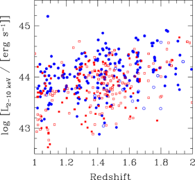
Figure 2.— Redshift vs. absorption-corrected 2–10 keV luminosity of X-ray-selected AGNs in the SXDS. Filled circles and squares represent broad-line and narrow-line AGNs with spectroscopic identification, respectively. Broad-line (narrow-line) AGN candidates with photometric redshifts are shown with open circles (open squares).

Table 1Summary of the SXDS broad-line AGN sample

	N	${\rm{N}}_{\rm{soft}}$	${\rm{N}}_{\rm{hard}}$	Note
X-ray sources	945	781	584	within deep Suprime-cam image coverage
AGN candidates	896	733	576
Optical spec. observed	590	517	396	among the 896 AGN candidates
FMOS spec. observed	851	704	548	among the 896 AGN candidates
Spec. identified	586	514	397
Mg II broad-line	186	181	137	z range 0.489 - 2.329
H$\alpha$ broad-line	81	78	68	z range 0.634 - 1.655
Mg II and H$\alpha$ broad-line	52	51	44

Note. —

Table 2Summary of SXDS AGNs in the redshift range $1.18\leq{\rm{z}}\leq 1.68$

	N	${\rm{N}}_{\rm{soft}}$	${\rm{N}}_{\rm{hard}}$
Broad-line AGN sample
Total (excluding broad-line AGNs with photometric redshift)	118	112	90
$M_{\rm BH}$ with Mg II broad-line FWHM	93	90	67
Additional $M_{\rm BH}$ with H$\alpha$ broad-line FWHM	23	21	21
Spectroscopically-identified broad-line AGN w/o Mg II or H$\alpha$ measurement	2	1	2
Broad-line AGN in the redshift range identified with photometric redshift	10	10	5
Narrow-line AGN sample
Total	158	120	101
Spectroscopically-identified narrow-line AGN	66	52	41
Narrow-line AGN with photometric redshift	92	68	60

A sample of $z\sim 1.4$ AGNs is constructed from X-ray observations of the SXDS field (Ueda et al., 2008). The field was observed with the XMM-Newton covering one central $30^{\prime}$ diameter field at a depth of 100ks exposure and six flanking fields with 50ks exposure time each (Ueda et al., 2008). From summed images of pn, MOS1, and MOS2 detectors, there are 866 and 645 sources detected in the 0.5–2 keV (soft) and 2–10 keV (hard) bands, respectively, with a detection likelihood, which is determined by point spread function fitting, larger than 7, which corresponds to a confidence level of 99.9%. In this paper, only X-ray sources in the region covered with deep optical imaging data taken with Suprime-cam on the Subaru telescope (Furusawa et al., 2008) are considered. There are 781 and 584 sources in the soft- and hard-bands, respectively. Once Galactic stars and clusters of galaxies candidates are removed, 733 (576) sources remain as AGN candidates. Hereafter we call the former (latter) sample the soft- (hard-) band sample. The detection limit of the survey corresponds to a flux of $6\times 10^{-16}$ erg s^-1 cm^-2 ($3\times 10^{-15}$ erg s^-1 cm^-2) in the soft (hard) band. The area covered with the flux limit is 0.05 deg², and 1.0 deg² is covered at the flux limit of $4\times 10^{-15}$ erg s^-1 cm^-2 in the soft band. Considering sources common to both samples, there are 896 unique AGN candidates in total (see Table 1).

In order to identify the X-ray sources spectroscopically, optical observations were conducted with various multi-object spectrographs on 4m- and 8m-class telescopes. The optical spectroscopic observations cover 590 out of the 896 sources in total. Even though the observations do not cover the entire sample, they are not heavily biased toward a specific type of object, since we do not use any further discrimination such as color in the target selection in most of the observations. Details of the observations are summarized in Akiyama et al. (2012, in preparation).

Additional intensive NIR spectroscopic observations were made with the Fiber Multi Object Spectrograph (FMOS) on the Subaru telescope (Kimura et al., 2010). This instrument can observe up to 200 objects simultaneously over a 30^′ diameter FoV in the cross-beam switching mode with two spectrographs. The spectrographs cover the wavelength range between 9000Å and 18000Å with spectral resolution of $R\sim 800$ at $\lambda\sim 1.55\mu$m in the low-resolution mode. A total of 851 sources were observed with this setup during guaranteed, engineering and open-use (S11B-098 Silverman et al. and S11B-048 Yabe et al.) observations. The optical and NIR observations spectroscopically identify 586 out of the 896 sources. The optical and NIR spectra obtained in the identification observations are used for the broad-line width measurements described in the next section.

The remaining 310 sources cannot be identified spectroscopically, mostly because of their faintness. Most of them are fainter than $i=23.5$ magnitude. For such objects, photometric redshifts have been estimated using the HyperZ photometric redshift code (Bolzonella et al., 2000) with galaxy and QSO Spectral Energy Distribution (SED) templates. Photometric data in 15 bands covering from 1500Å to 8.0$\mu$m are used in the estimation. In order to reduce the number of AGNs with significantly different photometric redshift from spectroscopic one (”outliers”), we apply two additional constraints in addition to the $\chi^{2}$ minimization considering the properties of the spectroscopically-identified AGNs. First one is that the objects with stellar morphology in the deep optical images are $z>1$ broad-line AGNs. Almost all X-ray sources with stellar morphology are identified with broad-line AGNs at $z>1$ in SXDS. They show a bright nucleus and their observed optical light is dominated by the nuclear component. Second one is the absolute magnitude range of the galaxy and QSO templates. Considering the absolute magnitude range of spectroscopically-identified broad-line and narrow-line AGNs, we limit the $z$-band absolute magnitude range of the galaxy (QSO) template between $M_{z}=-20.0--25.0$ (mag) ($M_{z}=-22.0--26.5$ (mag)).

The accuracy of the photometric redshifts are examined by comparing them with the spectroscopic redshifts. The median of $\Delta z/(1+z_{\rm spec})$ is 0.06 for the entire sample. We further examine the accuracy by the normalized median absolute deviation (NMAD; $\sigma_{z}$) following Brammer et al. (2008). For the entire sample, $\sigma_{z}$ is 0.104, which is larger than that of the photometric redshift estimations for X-ray-selected AGNs with medium band filters (Cardamone et al., 2010; Luo et al., 2010). The $\sigma_{z}$ for broad-line AGNs (0.201) is larger than that for narrow-line AGNs (0.095). This is because there is no strong feature in the SEDs of the broad-line AGNs except for the break below Ly$\alpha$.

From the photometric redshift determination, not only their photometric redshifts, but also their types of SED can be constrained. For spectroscopically identified AGNs, there is a good correlation between the spectral type and the best-fit SED type; narrow-line and broad-line AGNs are fitted well with galaxy and QSO templates, respectively. Therefore, we classify objects fitted better with the QSO templates as broad-line AGNs and the others as narrow-line AGNs. The classification does not perfectly match the spectroscopic classification: in the redshift range, 10 out of 66 (31 out of 118) spectroscopically-identified narrow-line (broad-line) AGNs are photometrically classified as broad-line (narrow-line) AGNs. The SEDs of the spectroscopically-unidentified objects suggest that most of them are obscured narrow-line AGNs above redshift 1. For 6 objects, no photometric redshift can be estimated because they are detected only in a few bands. They are faint and are unlikely to be broad-line AGNs in the redshift range between $1.18$ and $1.68$. Further details of the photometric redshift determination is discussed in Akiyama et al. (2012, in preparation).

In this paper, for objects with spectroscopic identification, we designate objects as broad-line AGNs if they show either Mg II$\lambda\lambda 2796,2803$ or H$\alpha$ emission lines with width greater than 1000 km s^-1. We estimate black hole mass of the broad-line AGNs with either broad Mg II or H$\alpha$ line. The threshold is narrower than typical threshold used to discriminate broad-line AGNs (1500 or 2000 km s^-1). We determine the threshold considering the distribution of the FWHM of the broad-line AGNs in the local universe (Hao et al., 2005; Stern & Laor, 2012). The broad-line AGNs with the line FWHM close to the threshold correspond to the narrow-line Seyfert 1s. Broad Mg II and H$\alpha$ lines are detected for 186 and 81 AGNs respectively, with redshifts in the range between $0.5$ and $2.3$. For 52 objects, both broad Mg II and H$\alpha$ lines are detected. For 29 objects, a broad-line is only detected in H$\alpha$. This is mostly due to the lack of optical spectra. Only 4 AGNs (SXDS0215, SXDS0387, SXDS0527, SXDS0728) with broad H$\alpha$ line show no broad Mg II line, although their optical spectra cover the Mg II wavelength region and are deep enough to detect continuum emission. Such AGNs are thought to be moderately affected by dust extinction and we correct for this in the determination of their continuum luminosity for the black hole mass and the intrinsic bolometric luminosity estimates. Details are given in Section 3 and 4.

For the derivation of the broad-line AGN BHMF, we limit the sample to the redshift range between 1.18 and 1.68. The FMOS $H$-band observation covers the broad H$\alpha$ line for AGNs in the redshift range. Considering the typical detection limit for the broad H$\alpha$ line in this redshift range ($L_{\rm H\alpha}=2\times 10^{42}$ (erg s^-1)), we expect a broad H$\alpha$ can be detected for broad-line AGNs brighter than $L_{\rm 2-10~{}keV}=3\times 10^{43}$ (erg s^-1), if they have the H$\alpha$ to hard X-ray luminosity ratio typical of broad-line AGNs (Ward et al., 1988). Photometric redshift estimates suggest 10 of the unidentified sources can be broad-line AGNs in this redshift range. All but one of the 10 candidates have estimated hard X-ray luminosity larger than $3\times 10^{43}$ (erg s^-1). But, 8 of the 10 broad-line AGN candidates do not show a broad-line in the FMOS observations. Considering the uncertainty of photometric redshift for broad-line AGNs, we expect they are broad-line AGNs at outside of the redshift range. However, there is a 0.4 dex scatter between the $L_{\rm 2-10~{}keV}$ and $L_{\rm H\alpha}$(Ward et al., 1988), and it is still possible that they have weaker broad H$\alpha$ line than the typical broad-line AGNs. Furthermore, additional one broad-line AGN candidate does not have broad-line in the optical spectroscopy, it may also be a broad-line AGN at outside of the redshift range. Considering the non-detection of broad-line in the observed wavelength range, we do not include the 10 photometric candidates of broad-line AGNs in the redshift range in the derivation of the BHMF and ERDF below. The numbers of X-ray-selected AGNs in the redshift range are summarized in Table 2. The median redshift of the sample is 1.43.

The redshift distribution of the sample is shown in Figure 1 for the redshift range 0.5 to 2.5. The thick solid line shows the redshift distribution of the X-ray AGNs with spectroscopic or photometric redshifts. The dashed line shows the distribution of spectroscopically-identified AGNs. The thin solid line shows the distribution for broad-line AGNs with spectroscopic redshifts. The dotted line is the distribution for broad-line AGNs that have black hole mass estimates with either broad Mg II or H$\alpha$ emission lines.

In Figure 2, the absorption-corrected 2–10 keV luminosity of AGNs are shown as a function of redshift. Following Ueda et al. (2003), we assume the intrinsic shape of the X-ray spectrum and estimate the intrinsic column density from the observed hardness ratio and redshift. The intrinsic X-ray spectrum of AGNs is modeled by a combination of a power-law component with high-energy cut off $E^{-\Gamma}\times\exp{(-E/E_{c})}$ and a reflection component. A photon index $\Gamma$ of 1.9 and cutoff energy $E_{c}$ of 300 keV are assumed. We calculate the reflection component with the “pexrav” (Magdziarz & Zdziarski, 1995) model in the XSPEC package assuming a solid angle of 2$\pi$, an inclination angle of $\cos i=0.5$, and solar abundance of all elements. Strength of the reflection component is about 10% of the direct component just below 7.1 keV. The intrinsic SEDs are modified with intrinsic photo-electric absorption described by a hydrogen column density, $N_{\rm H}$. The $N_{\rm H}$ value of each object is evaluated from the observed 0.5–2 keV and 2–4.5 keV hardness ratio. The absorption-corrected luminosity in the 2–10 keV band is derived from the observed 2–10 keV count-rate by correcting for the photo-electric absorption. For objects only detected in the 0.5–2 keV band, the count-rate in that band is used instead of the 2–10 keV count-rate. Most of the broad-line AGNs have a hardness ratio consistent with no significant absorption and the required correction is small. Only 5 out of the 215 broad-line AGNs have $\log N_{\rm H}$ as large as $23$; for these the correction in luminosity is as large as 0.5 dex.

The absorption-corrected 2–10 keV luminosity of AGNs distribute between $L_{\rm 2-10~{}keV}=10^{43}$ and $10^{45}$ (erg s^-1) in the redshift range of $z=1-2$. The SXDS AGNs cover the most important part of the accretion growth of the SMBHs. AGNs in the luminosity range dominate the hard X-ray luminosity density of the Universe in the redshift range, furthermore, the hard X-ray luminosity density as a function of redshift peaks at $z=1$ (Aird et al., 2010).

3. LINE WIDTH AND LUMINOSITY MEASUREMENT

3.1. Method for Black Hole Mass Estimation

Assuming that the scaling relationship between luminosity and broad-line region size derived by reverberation mapping for local broad-line AGNs is applicable to broad-line AGNs at high-redshifts, black hole masses of broad-line AGNs can be estimated from their continuum luminosities and line widths of the broad lines. We estimate the black hole mass of $z\sim 1.4$ broad-line AGNs with Mg II broad-line widths measured in the optical spectra. As the optical spectroscopy does not cover the entire sample, we supplement these with H$\alpha$ broad-line widths measured in the NIR spectra. In this subsection, we first introduce the equation used to estimate the black hole mass.

There are several calibrations available for the black hole mass estimation using the Mg II broad line (McLure & Jarvis, 2002; McLure & Dunlop, 2004; McGill et al., 2008; Vestergaard & Osmer, 2009; Wang et al., 2009; Shen et al., 2011; Rafiee & Hall, 2011). We use the black hole mass estimate from the Mg II broad-line FWHM calibrated by broad-line QSOs in the SDSS DR3 (Vestergaard & Osmer, 2009). The estimation is consistent to within 0.1 dex of the H$\beta$ and C IV mass estimates with single-epoch spectra. They are calibrated to the black hole mass from the reverberation mapping (Vestergaard & Peterson, 2006). It needs to be noted that the black hole mass determined with the single-epoch H$\beta$ spectrum typically has scatter of 0.4-0.5 dex around that from the reverberation mapping (Vestergaard & Peterson, 2006). Park et al. (2012) also estimate the uncertainty of the single-epoch black hole mass to be 0.4-0.5 dex. Furthermore, if AGNs are close to the Eddington limit, the influence of radiation pressure may cause an underestimation of the black hole mass by $0.5$ dex (Marconi et al., 2008).

Because the 3000Å monochromatic luminosity is available for most of the broad-line AGNs with spectroscopic observations, we use the following equation from Vestergaard & Osmer (2009) incorporating the 3000Å monochromatic luminosity, $L_{\lambda 3000}$.

$$M_{\rm BH}[M_{\sun}]$$ (1)

$$= 10^{6.86}\left[\frac{\rm FWHM_{\rm MgII}}{1000{\hskip 2.84526pt}\rm{km\ s^{-1}}}\right]^{2}\left[\frac{\lambda 3000L_{\lambda 3000}}{10^{44}{\hskip 2.84526pt}{\rm{erg\ s^{-1}}}}\right]^{0.5}.$$

In this calibration, the FWHM of broad Mg II line, FWHM_MgII, is measured by fitting multiple Gaussians to the Mg II emission line profile. Vestergaard & Osmer (2009) remove narrow-line component of Mg II if necessary (Vestergaard et al., 2011). In other calibrations, such as McLure & Jarvis (2002) and McLure & Dunlop (2004), fit the Mg II profile with a single broad-line and narrow-line components. Rafiee & Hall (2011) use the line dispersion, $\sigma$, of the broad-line because $\sigma$ correlates more tightly with the delay observed in reverberation mapping, i.e. size of the broad-line region, than with the FWHM (Peterson et al., 2004).

In Equation (1), the broad-line region size $R$ is assumed to follow $L^{\alpha}$ with $\alpha$ of 0.5, which is equivalent to assuming that the broad-line regions of various AGNs can be described as having similar ionization states, ionizing photon spectra and electron densities. The value of $\alpha$, based on reverberation mapping results for H$\beta$ broad-lines, is determined to be 0.47, $0.62\pm 0.14$, and $0.518\pm 0.039$ (McLure & Jarvis, 2002; McLure & Dunlop, 2004; Bentz et al., 2006), respectively, all consistent with $\alpha$ of 0.5 within the uncertainties.

Regarding the coefficient for the virial product ($\epsilon$ of $M_{\rm BH}=\epsilon{\rm FWHM_{H\beta}}^{2}L^{0.5}$ or $f$ of $M_{\rm BH}=f\sigma_{H\beta}^{2}L^{0.5}$), Equation (1) is based on the calibration done by Onken et al. (2004) ($\epsilon$ of 1.4 or $f$ of 5.5) assuming the estimated $M_{\rm BH}$ of local broad-line AGNs from reverberation mapping and their bulge velocity dispersions follow the black hole mass and the bulge velocity dispersion relation of non-active galaxies in the local Universe. The coefficient is consistent with that derived with local Seyfert 1 galaxies ($f=5.2$; Woo et al., 2010). Recent calibration shows broad-line AGNs hosted in barred galaxies are consistent with significantly smaller values ($f=2.3$; Graham et al., 2011), but the range of black hole mass of the barred galaxies is smaller than the current sample, and non-barred galaxies with larger $M_{\rm BH}$ is consistent with $f\sim 5.4$ (Graham et al., 2011), thus we use Equation (1).

The optical spectroscopic observations do not cover all of the broad-line AGNs at $z=1.18-1.68$; 25 out of 118 spectroscopically-identified broad-line AGNs in the redshift range do not have Mg II data. Therefore, we also utilize the H$\alpha$ FWHM in addition to the Mg II FWHM; additional 23 broad-line AGNs have H$\alpha$ broad-line data. Although the FMOS spectra cover H$\beta$ in $J$-band, the strength of the H$\beta$ broad-line is 3 times or more weaker than the H$\alpha$ broad-line and the uncertainty of the FWHM of the broad H$\beta$ is significantly larger than that of the broad H$\alpha$ line. Therefore, we do not use the H$\beta$ FWHM. Because ionization potentials of hydrogen and Mg II are similar, Balmer and Mg II$\lambda\lambda 2796,2803$ broad lines are expected to be emitted in a similar region. A detailed photoionization model calculation indicates that the equivalent widths of H$\alpha$ and Mg II lines have a similar dependency on the cloud density and ionization parameter, i.e., they are emitted from similar broad-line clouds (Korista et al., 1997). Considering this similarity, we use the same black hole mass equation employed for Mg II FWHM above for H$\alpha$ FWHM, after correcting for a small systematic difference between Mg II FWHM and H$\alpha$ FWHM, as detailed below. We do not use the scaling relation calibrated for H$\alpha$ broad-line (Greene & Ho, 2005) in order to be consistent within our sample. The derivation of the 3000Å monochromatic luminosity is discussed in Section 3.4.

3.2. Mg II Line Width Measurements with Optical Spectrum

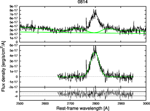
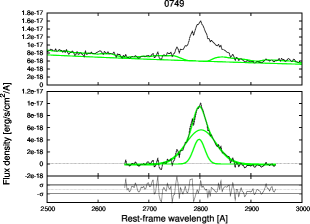
Figure 3.— Examples of broad Mg II fitting. Upper panels show the observed data (thin solid line) and the best fit model from the power-law continuum and Fe II fitting (thick solid line). Power-law component of the best fit model is also shown separately. Middle panels show the results of the broad Mg II line fitting. Pure Mg II component after subtracting the power-law continuum and Fe II components and best fit model from the Mg II fitting are shown with thin solid line and thick solid line, respectively. Each component of the best fit model is also shown. Only the wavelength range used for the broad-line fitting is plotted. Bottom panels show the residual after fitting. Left) SXDS0814 with single broad-line, and right) SXDS0749 with 2 components.

Figure 4.— FWHMs of the broad Mg II emission line determined after Fe II fitting with with VW01 and T06 Fe II templates. The dashed line shows the equal FWHM line.

Optical spectra of the AGNs were obtained with various instruments on 4-8m class telescopes such as 2dF on the Anglo-Australian Telescope, VIMOS and FORS on the Very Large Telescope, FOCAS on the Subaru telescope, DEIMOS on the Keck telescope, and IMACS on the Magellan telescope. Most of them were obtained with spectral resolution of $R\sim 250-500$. Details of the observations are described in Akiyama et al. (2012, in preparation). The optical spectroscopic data were reduced using standard procedures and are corrected for the dependence of the sensitivity on wavelength with standard star observations. We further correct the normalization of the spectra to match the observed $R$-band magnitudes in the deep Suprime-cam images. The optical photometric data are corrected for the Galactic extinction in the SXDS field ($A_{R}$ of 0.07 mag). We do not correct the optical spectroscopic data for the wavelength dependence of the Galactic extinction which is negligibly small. This correction does not affect the line width measurement, but affects the continuum flux measurement. The normalization can be affected by the variability of broad-line AGNs between the epochs of the imaging and the spectroscopic observations. Typically there is one year gap between the imaging and spectroscopic observations. The structure function of optical variability of QSOs (Cristiani et al., 1996) suggests that there can be 0.2 mag variation during the time lag on average. Therefore, the uncertainty of $M_{\rm BH}$ due to the time-variation of AGNs is expected to be 0.04 dex.

In order to determine the Mg II FWHMs of broad-line AGNs, it is necessary to consider Fe II emission lines as well as the power-law continuum component in the UV wavelength range. Because there are many broad Fe II emission lines in the wavelength range, they look like an additional continuum component to the power-law continuum of broad-line AGNs. We use a Fe II template derived from the UV spectrum of the narrow-line Seyfert 1 galaxy, I Zw 1 (Vestergaard & Wilkes, 2001). This template covers the rest-frame wavelength range between 1074Å and 3089Å. We do not include the Balmer continuum in the fitting, because the wavelength coverage is not wide enough to constrain its contribution. The ignorance of the Balmer continuum does not affect the Mg II FWHM measurements significantly, but the luminosity of the power-law continuum can be overestimated by 0.12 dex (Shen & Liu, 2012).

A fit to the power-law continuum, Fe II emission lines, and Mg II emission line is carried out as follows. First, we determine the normalization of Fe II and continuum component using $\chi^{2}$ minimization in the two rest-frame wavelength ranges, 2500-2700Å and 2900-3000Å in which Mg II broad-line component is negligible. These are close to the pure Fe emission windows nos.9 and 10 in Vestergaard & Wilkes (2001). We vary the line width of the Fe II emission lines from 1000 km s^-1 to 15000 km s^-1 with a step size of 250 km s^-1 by convolving a Gaussian profile with the Fe II template which has a velocity width of 900 km s^-1. We assume a constant line width for all Fe II emission lines. The scaling of the Fe II emission is changed from 0 to 100% of the observed continuum level with a step size of 0.01%. The continuum component is modeled with a power-law spectrum ($f_{\nu}\propto\nu^{-\alpha}$). The observed wavelength ranges affected by strong night sky lines (5555-5605Å and 6270-6320Å) are removed in the fitting. Because some optical spectra do not have noise level estimation from the standard reduction method, we estimate the noise level for each spectrum as follows. Considering that the noise level does not vary significantly within the observed wavelength range, we use a constant noise level for the entire wavelength range. In the first stage of the fitting, we use the standard deviation determined within the wavelength range as the noise level. Subsequently, we determine the noise level from the rms of the residual of the first fitting, and carry out the final fit for the continuum. The noise level is used for the Mg II line profile fitting as well. Examples of continuum fits are shown in the upper panels of Figure 3.

By subtracting the Fe II emission and power-law continuum components, the Mg II broad-line component is extracted. Then we measure the FWHM of the Mg II broad-emission line after fitting its line profile with multiple Gaussians using $\chi^{2}$ minimization. In the fitting, we do not consider the doublet component of Mg II$\lambda\lambda 2796,2803$, because the separation is small and does not affect the measured width of the broad Mg II line. We use mpfit package for python for $\chi^{2}$ minimization (Markwardt, 2009). Mpfit uses Levenberg-marquardt algorithm to derive the best fit parameters. For some objects, the Mg II line profile cannot be described with a single Gaussian component. In such cases, we consider up to three broad Gaussians for the broad line. If necessary, we include narrow doublet absorption lines. Sometimes we also include a narrow Gaussian component to remove artificial spiky noise features. Because no object shows a significant existence of narrow Mg II line, we do not include a narrow-emission line component in the fitting. No inclusion of the narrow-line component differs from the fitting method used in most of the literatures such as McLure & Jarvis (2002). Once the pure Mg II broad-line component is fitted with the multiple Gaussian components, the FWHM of the broad Mg II line is measured with the best fit profile constructed by combining the multiple Gaussians. We do not include absorption lines in the combination. We introduce multiple Gaussian components in order to reproduce the observed Mg II broad-line profile smoothly and here we are not concerned with the physical meaning of the difference from the single Gaussian profile. Examples of the resulting Mg II broad-line fitting are shown in the middle and bottom panels of Figure 3. Because the spectra are obtained with various instruments, the spectral resolution of data varies from object to object. The spectral resolution is evaluated for each spectrum by using line width of the arc lamp spectrum or night sky emission lines. The measured FWHMs are corrected for the intrinsic spectral resolution.

The uncertainty of the FWHM values for the combined multiple Gaussian profile is not available from the fitting with mpfit package (uncertainty is only available for each Gaussian component). Therefore we evaluate the uncertainty for the FWHM of each object from the rms scatter of FWHMs measured in mock spectra constructed from the best fit profile of the object. We construct the mock spectra as follows. First, the best fit multi-Gaussian model is shifted by several pixels in wavelength from its original position. Then the shifted model profile is combined with the residual of the original fitting. By monotonically increasing the shift and changing the sign of residual in each pixel randomly, we construct 100 mock spectra. The mock spectra are fitted in the same way as the original data and FWHMs are measured. Finally the rms scatter of the derived FWHMs is used as the uncertainties of the FWHM measurement. For AGNs whose Mg II broad-line is fitted with single Gaussian component, we compare the uncertainties derived from the $\chi^{2}$ statistics and from the scatter of the mock measurements. They are consistent with each other, although the rms scatter of the mock measurements is slightly smaller than the uncertainties from the $\chi^{2}$ statistics. Hereafter, we use the uncertainty derived with the scatter of the mock measurements. The fitting results are summarized in Table 3. Column 4 of the table describes the model used for each object; ”OneBL”, ”TwoBL” and ”ThreeBL” indicate fitted with one, two and three broad lines respectively. ”OneBLOneAbs” indicates a model with one broad and one absorption line.

For the Mg II profile fitting, we also use the specfit software in the stsdas package of IRAF. This package uses Marquardt algorithm or simplex algorithm for $\chi^{2}$ minimization. We compare the results obtained with mpfit and specfit for each object. The rms scatter of the difference in FWHMs from the two measurements is 0.06 dex. The resulting uncertainty in $M_{\rm BH}$ due to the scatter is 0.12 dex. We use the results obtained with mpfit hereafter.

The measured FWHM of Mg II broad-line can be affected by the template used for the Fe II fitting. For the Fe II fitting, we use the empirically derived Fe II template from Vestergaard & Wilkes (2001) (VW01 template). There is no Fe II emission in the wavelength range between 2770Å and 2820Å in the template. Tsuzuki et al. (2006) also derived the Fe II template (T06 template) from UV and optical spectra of I Zw 1. Utilizing the wide wavelength coverage available, they fit the continuum with a power-law and Balmer continuum and also utilize the H$\alpha$ line profile for removing the Mg II line component. The important difference between the two templates is the Fe II contribution to the blue wing of the broad Mg II line. In the T06 template, the excess wing seen on the blue side of the Mg II line of I Zw 1 compared with its H$\alpha$ line profile is regarded as a contribution from the Fe II emission line at around 2790Å. In order to examine the effect of different Fe II templates on the FWHM measurement, we also apply the Mg II emission line fitting process described above using the T06 template for 95 objects whose broad Mg II lines are fitted well with one broad-line component with the VW01 template. Figure 4 compares the $\log$ FWHMs values derived with the two templates. There is a systematic offset of 0.04 dex; the FWHMs derived with the T06 template are systematically smaller than those with the VW01 template. The rms scatter of the difference is 0.05 dex after removing the systematic offset. The resulting systematic uncertainty of $M_{\rm BH}$ is 0.08 dex. In order to compare the broad-line AGN BHMFs from literature, we follow the same fitting procedure using the VW01 template, but it needs to be noted that the FWHMs can have a systematic uncertainty due to the Fe II template difference.

Table 3Broad-line fitting results for the broad-line AGNs

			Mg II		H$\alpha$
ID	z	log[$L_{\rm HX}$	FWHM	model	FWHM	model	$\log[\lambda 3000L_{\lambda 3000}$	$R-i$
		/ [erg $\rm{s}^{-1}$] ]	[km $\rm{s}^{-1}]$		[km $\rm{s}^{-1}$]		/ [erg $\rm{s}^{-1}$] ]	[mag]
0010	1.225	44.05	5341 $\pm$ 12	TwoBL	5135 $\pm$ 116	OneBL	44.89	$-$0.04
0018	1.452	44.42	$\cdots$	$\cdots$	5488 $\pm$ 92	BLNL	45.16	$-$0.02
0019	1.447	44.66	4823 $\pm$ 312	OneBL	$\cdots$	$\cdots$	45.41	$-$0.06
0023	1.534	44.14	$\cdots$	$\cdots$	5602 $\pm$ 112	OneBL	45.10	0.48
0027	2.067	43.75	4136 $\pm$ 1499	TwoBL	$\cdots$	$\cdots$	45.85	0.27
0034	0.952	43.55	4286 $\pm$ 1005	TwoBL	2459 $\pm$ 123	TwoBL	44.72	$-$0.15
0036	0.884	44.16	3326 $\pm$ 22	TwoBL	2790 $\pm$ 50	TwoBL	45.24	0.25
0037	1.202	43.81	4516 $\pm$ 70	TwoBL	$\cdots$	$\cdots$	44.45	$-$0.06
0050	1.411	44.03	2046 $\pm$ 120	OneBL	1800 $\pm$ 68	OneBL	44.80	0.14
0056	1.260	44.19	$\cdots$	$\cdots$	8171 $\pm$ 456	BLNL	44.74	$-$0.03

3.3. H$\alpha$ Line Width Measurements from NIR Spectrum

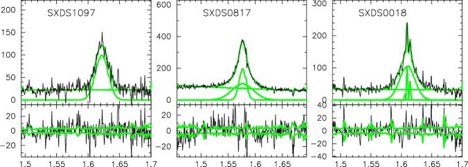
Figure 5.— Examples of broad H$\alpha$ fitting. Upper panels show the observed data (thin solid line) and the best fit model with each component (thick solid lines). Lower panels show the residual from the fitting (thin solid line). Thick solid lines in the panel enclose the estimated $1\sigma$ noise level at each wavelength. Left) SXDS1097 with single broad-line, middle) SXDS0817 with 2 broad-lines, and right) SXDS0018 with broad-line and narrow H$\alpha$ and [N II]$\lambda\lambda 6548,6583$ lines.

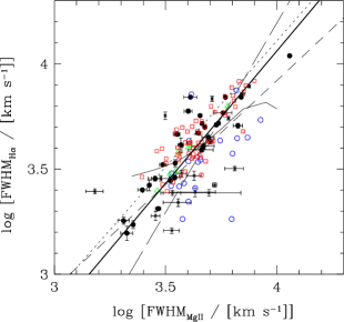
Figure 6.— Comparison between FWHMs of H$\alpha$ and Mg II broad-lines for SXDS AGNs. Filled circles and crosses represent broad-line AGNs brighter and fainter than $L_{\rm 2-10~{}keV}=10^{44}$ erg s^-1, respectively. The thick solid line represents the BCES bisector fitting result for the SXDS AGNs. Open squares, triangles, and circles are AGNs from Shen & Liu (2012), Greene et al. (2010b), and McGill et al. (2008), respectively. The relationships between the Mg II and H$\beta$ FWHMs from McLure et al. (2002) (short dashed line), Onken & Kollmeier (2008) (thin solid line), Wang et al. (2009) (dotted line), and Croom et al. (2011) (long dashed line) are shown after converting H$\beta$ FWHM to H$\alpha$ FWHM.

The NIR spectra of X-ray sources obtained with FMOS were reduced with the pipeline data reduction software, FIBRE-pac (Iwamuro et al., 2012). The resulting 1-d spectra are corrected for atmospheric absorption and sensitivity dependence on wavelength using relatively bright F-G type stars observed simultaneously with the targets. Because we do not use the absolute flux of the continuum component, we do not apply further correction for normalization based on the photometry. Noise level of each spectrum is also estimated in the pipeline data reduction software.

The profile of the broad H$\alpha$ line is fitted with mpfit in a similar way for broad Mg II component. The possible existence of the narrow emission lines of H$\alpha$ and [N II]$\lambda\lambda$6583,6548 makes the fitting more complicated than for Mg II broad line. We include the narrow emission lines in the fitting only if a prominent narrow emission feature, such as asymmetric profile due to the 1:3 flux ratio of [N II] lines, is observed. For the broad H$\alpha$ component, we use up to two Gaussians to fit their profile. In the fitting process, we assume a constant continuum component because the continuum of the observed NIR spectra does not show significant tilt in the region around H$\alpha$ emission line. Due to the existence of the OH suppression mask, the strength of the narrow emission line can be underestimated even after the sensitivity correction process if the narrow emission line is close to the masked wavelength. We apply the fitting procedure taking into account the underestimation due to the optical masking and the sensitivity correction process. The details of the fitting procedure are described in Yabe et al. (2012). It needs to be noted that the effect of OH suppression mask only affects the narrow-emission line and the effects on the broad-emission lines and continuum are negligible. Examples of H$\alpha$ fitting are shown in Figure 5.

The uncertainty in the FWHM measurements of the broad H$\alpha$ emission line is evaluated in the same way as for the broad Mg II emission lines. We construct 10 model spectra by adding shifted best fit multi-Gaussian model to the residual of the fitting. Then, the same fitting procedure is applied to the model spectra and the rms scatter of the measured FWHMs is used as the uncertainty of the FWHM measurement. In this fitting process we also take into account the effect of the OH suppression mask.

The resulting FWHM of the broad H$\alpha$ emission is compared with that of the broad Mg II line for broad-line AGNs with FWHM measurements for both lines in Figure 6. We remove Mg II FWHMs of 4 broad-line AGNs (SXDS0590, SXDS0630, SXDS0790, and SXDS0969), because the signal-to-noise ratios of their Mg II spectra are much lower than those for their H$\alpha$ spectra. Therefore, 48 broad-line AGNs are plotted in the figure. The sample is divided with the absorption-corrected X-ray luminosity. Broad-line AGNs that are brighter (fainter) than $L_{\rm 2-10keV}=10^{44}$ erg s^-1 are marked with filled squares (crosses). The measured FWHMs of the broad Mg II and H$\alpha$ lines roughly follow the equality line. However, there may be a tendency that broad-line AGNs with lower luminosity have systematically smaller broad H$\alpha$ FWHM than broad Mg II line. The distribution is broadly consistent with those of broad-line AGNs measured in the literature. We show the Mg II and H$\alpha$ FWHMs of individual broad-line AGNs from Shen & Liu (2012), Greene et al. (2010b), and McGill et al. (2008). The samples of Shen & Liu (2012) and Greene et al. (2010b) are luminous broad-line AGNs with $L_{\rm bol}$ of $10^{46-48}$ erg s^-1 at $z=1-2$. On the contrary, the McGill et al. (2008) sample covers broad-line AGNs with $L_{\rm bol}$ of around $10^{45}$ erg s^-1 at $z\sim 0.3$. The distribution of the former samples are consistent each other and follow similar trend of the SXDS luminous broad-line AGNs. The latter sample has systematic offset from the former samples and shows smaller H$\alpha$ broad-line FWHM than Mg II FWHM. The trend is similar to that seen in the SXDS less-luminous broad-line AGNs.

We determine the relationship between the Mg II and H$\alpha$ FWHMs applying a BCES (Bivariate Correlated Error and intrinsic Scatter) bisector regression analysis (Akritas & Bershady, 1996) to the 48 broad-line AGNs including both luminous and less-luminous AGNs. Considering the size of the sample, we do not divide the sample by luminosity in the analysis. The resulting relationship is

$$\log {\rm FWHM}_{\rm MgII}$$

$$= (0.795\pm 0.075)\times\log{\rm FWHM}_{\rm H\alpha}+(0.771\pm 0.273).$$

The rms scatter of $\log{\rm FWHM}_{\rm MgII}$ determined with the above relationship using the measured $\log{\rm FWHM}_{\rm MgII}$ is 0.11 dex with a resulting uncertainty for $\log M_{\rm BH}$ of 0.22 dex. The less luminous broad-line AGNs show systematic offset of 0.1 dex on average from the relation.

The relationship between the FWHMs of the H$\beta$ and Mg II broad-lines from McLure & Jarvis (2002) (short dashed line), Onken & Kollmeier (2008) (thin solid line), Wang et al. (2009) (dotted line), and Croom (2011) (long dashed line) are also shown in the figure. These relationships for the H$\beta$ FWHMs are converted to those for the H$\alpha$ FWHMs using the relationship between the FWHMs of the broad H$\alpha$ and H$\beta$ lines determined from $z<0.35$ for local broad-line AGNs of SDSS (Eq.(3) of Greene & Ho, 2005). The relationship between the FWHMs of H$\alpha$ and H$\beta$ is consistent with a recent determination of Shen et al. (2008b) but is slightly offset from the relationship of Schulze & Wisotzki (2010). The distribution of SXDS broad-line AGNs is consistent with the relationship of McLure & Jarvis (2002) and Onken & Kollmeier (2008). The relationship of Croom (2011) has a steeper slope than the other relationships and follows the distribution of SXDS broad-line AGNs except for the objects with the largest FWHMs. The relationship of Wang et al. (2009) shows a systematic offset from the other relationships and the distribution of SXDS broad-line AGNs. The origin of the shift is unclear, but it is possible that Wang et al. (2009) use T06 Fe II template, and FWHM of Mg II is measured systematically smaller than other measurements with VW01 Fe II template (see Section 3.2).

We use the relationship shown as the Equation (2) to convert the H$\alpha$ FWHM to Mg II FWHM and the same black hole mass equation for Mg II FWHM is applied. In total, we use the H$\alpha$ FWHM measurements for 23 out of 116 broad-line AGNs at redshifts between 1.18 and 1.68.

3.4. 3000Å Monochromatic Luminosities

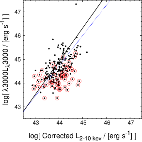
Figure 7.— Absorption corrected 2–10 keV luminosity vs. 3000Å monochromatic luminosity of the SXDS broad-line AGNs (filled circles). Broad-line AGNs redder than $R-i>0.3$ magnitude are marked with large open circles. The thick solid line indicates the relationship determined by Marconi et al. (2004). The dotted line shows the relationship determined with the BCES bisector analysis for broad-line AGNs bluer than $R-i<0.3$ magnitude.

For most of the objects, we derive 3000Å monochromatic luminosity using the best-fit power-law continuum component described in Section 3.2. We do not include the contribution of the Balmer continuum in the fitting, the 3000Å monochromatic luminosity can be overestimated by 0.12 dex (Shen & Liu, 2012). Optical spectra covering rest-frame 3000Å are not available for broad-line AGNs that only covered by the NIR spectroscopic data. We estimate their 3000Å monochromatic luminosity by interpolating multi-band photometry data. All of the broad-line AGNs are detected in the deep multi-band images obtained with Suprime-Cam. We derive their rest-frame 3000Å flux by interpolating the photometric measurements in the neighboring two bands around rest-frame 3000Å. The photometric data can include broad-emission lines and Balmer continuum as well, and the 3000Å luminosity may thus be affected by the broad-line component. In order to estimate this effect, we compare the 3000Å luminosity derived from normalized spectra and multi-band photometry for objects with both measurements. They are consistent each other within the rms of 0.10 dex and resulting uncertainty of $M_{\rm BH}$ is 0.05 dex. It needs to be noted that the optical spectra are normalized to match the $R$-band photometry from the imaging observations as described in Section 3.2, therefore the scatter only reflects the object-to-object variation of the strength of the broad-line components. For the estimation of the 3000Å monochromatic luminosity with the photometric data, the contribution from the Balmer continuum is not considered. Uncertainty associated with the variability of broad-line AGNs is already described in Section 3.2.

For mildly obscured broad-line AGNs, the 3000Å luminosity can be affected by dust extinction. Additionally for low-luminosity broad-line AGNs, the 3000Å luminosity can be affected by a host galaxy component. In such cases, the neither the 3000Å luminosity derived from the spectra nor the photometry is a good indicator of the intrinsic UV luminosity. In Figure 7, the monochromatic 3000Å luminosity and absorption corrected 2–10 keV luminosity of the broad-line AGNs are shown. In this figure, broad-line AGNs with $R-i$ color redder than 0.3 are marked with open circles. Those with a $R-i$ color of 0.3 are redder than the scatter of typical broad-line AGNs in the redshift range observed in SDSS (Richards et al., 2003). Hereafter, we designate broad-line AGNs with $R-i$ redder (bluer) than 0.3 as red (blue) broad-line AGNs. In the diagram, blue broad-line AGNs follow the relationship expected from the typical SEDs of broad-line AGNs as a function of intrinsic luminosity which is shown with solid line in the figure (Marconi et al., 2004). The dotted line in the figure shows the relationship determined with the BCES bisector analysis for the blue broad-line AGNs. In Marconi et al. (2004), the SEDs around 3000Å are described with a power-law with $\alpha=-0.44$ with $L_{\nu}\propto\nu^{\alpha}$ and a dependence on optical-to-X-ray flux ratio, $\alpha_{\rm OX}$, on optical luminosity of broad-line AGNs (Vignali et al., 2003) is considered. The $B$-band luminosity used in Marconi et al. (2004) is converted to a 3000Å monochromatic luminosity assuming a typical SED of broad-line QSOs ($1.549\times\lambda 4360L_{\lambda 4360}=\lambda 3000L_{\lambda 3000}$; Richards et al., 2006). The consistency of the distribution with this relation suggests that the blue broad-line AGNs have SEDs consistent with the optical-to-X-ray luminosity ratio, $\alpha_{\rm ox}$, dependence on luminosity for typical non-absorbed broad-line AGNs.

On the contrary, most of the red broad-line AGNs have a systematically fainter 3000Å monochromatic luminosity than the blue broad-line AGNs at the same absorption corrected 2–10 keV luminosity. The fainter 3000Å luminosity suggests that the red broad-line AGN are affected by mild dust absorption although most of them show a strong Mg II broad-line. Additionally, some of the red broad-line AGNs are brighter in their 3000Å luminosity. Most of them have the lowest absorption-corrected 2–10 keV luminosity and their red colors can be explained by contamination by a host galaxy component in the wavelength range. In both cases, the 3000Å luminosity is not a good indicator of intrinsic luminosity, thus we use absorption-corrected X-ray luminosity instead of the 3000Å monochromatic luminosity for the black hole mass estimation. We convert the absorption-corrected hard X-ray luminosity of the red broad-line AGNs to the intrinsic 3000Å monochromatic luminosity using the relationship derived by Marconi et al. (2004). Considering the scatter of blue broad-line AGNs around the relationship, we estimate the rms uncertainty of the intrinsic 3000Å monochromatic luminosity is 0.54 dex, which corresponds to 0.27 dex in the $M_{\rm BH}$ uncertainty. We use the 3000Å monochromatic luminosity derived from the hard X-ray luminosity of 59 red broad-line AGNs out of the 215 broad-line AGNs for the $M_{\rm BH}$ estimate. There are 26 red broad-line AGNs among the 116 broad-line AGNs in the redshift range between $1.18$ and $1.68$ where the broad-line AGN BHMF and ERDF are derived below.

In summary, 3000Å monochromatic luminosities are derived in three ways, from the power-law component of the fitting of optical spectrum, the optical broad-band photometry for broad-line AGNs only with the NIR spectrum, and hard X-ray luminosity for mildly-obscured or less-luminous broad-line AGNs. The resulting 3000Å monochromatic luminosities are summarized in Table 3.

4. Black Hole Mass, Bolometric Luminosity and Eddington Ratio

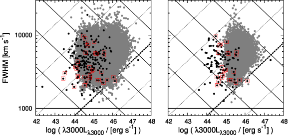
Figure 8.— Mg II FWHM vs. 3000Å monochromatic luminosities of SXDS broad-line AGNs (filled circles). Broad-line AGNs whose Mg II FWHMs are estimated based on H$\alpha$ FWHM are marked with large open squares. The solid lines indicate constant $M_{\rm BH}$ values for $M_{\rm BH}$ of $10^{7}$, $10^{8}$, $10^{9}$, $10^{10}$, and $10^{11}$ $M_{\sun}$ from bottom to top. The dotted lines show constant $\lambda_{\rm Edd}$ for $\log\lambda_{\rm Edd}$ of $1$, $0$, $-1$, $-2$, and $-3$ from bottom to top. The thick dotted line indicates $\log\lambda_{\rm Edd}$ of $0$. The thick solid line shows Mg II FWHM of 1000 km s^-1. SDSS DR5 broad-line AGNs that have a Mg II FWHM measurement (Shen et al., 2008a) are plotted as gray circles. Right) Same for broad-line AGNs at $z=1.18-1.68$ only.

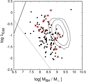
Figure 9.— Black hole mass versus Eddington ratio of broad-line AGNs at redshifts between 1.18 and 1.68. Broad-line AGNs whose Mg II FWHM are estimated from H$\alpha$ FWHM are marked with large open squares. The dotted line shows the relationship between $\log M_{\rm BH}$ and $\lambda_{\rm Edd}$ for a broad-line AGN with $L_{\rm 2-10~{}keV}=10^{43}$ erg s^-1, corresponding to the faintest object in the sample. The thick solid line indicate the constant Mg II FWHM of 1000 km s^-1. The distribution of the SDSS DR5 sample (Shen et al., 2008a) in the same redshift range is shown with the contours.

The distribution of broad-line AGNs in the measured Mg II FWHM vs intrinsic 3000Å monochromatic luminosity plane is shown in the left panel of Figure 8. Large open squares indicate the FWHMs that are estimated with the broad H$\alpha$ line and Equation (2). In the panel, the constant $M_{\rm BH}$ line derived from Equation (1) is shown with solid lines. From bottom to top, the lines correspond to $M_{\rm BH}$ of $10^{6}$, $10^{7}$, $10^{8}$, $10^{9}$, $10^{10}$, and $10^{11}$ $M_{\sun}$. The SXDS broad-line AGNs cover the $M_{\rm BH}$ range between $10^{7}\sim 10^{10}M_{\sun}$ with a median of $3.2\times 10^{8}M_{\sun}$.

Although we define broad-line AGNs as having FWHMs above 1000 km s^-1, a few objects have FWHMs between 1000 and 2000 km s^-1. In the panel, we compare the distribution with that of broad-line AGNs from SDSS DR5 (filled gray circles; Shen et al., 2008a). The 49,526 SDSS broad-line AGNs, which are selected with broad-line component whose FWHM is larger than 1200 km s^-1, are distributed between $z=0.3$ and $2.4$. Though there are far larger number of broad-line AGNs in the SDSS sample than in the SXDS sample, again only a negligible fraction of broad-line AGNs have FWHMs smaller than 2000 km s^-1. A similar rapid decrease of broad-line AGNs with FWHM smaller than 2000 km s^-1 is also reported by Hao et al. (2005) and Stern & Laor (2012). They select broad-line AGNs in the local Universe from SDSS galaxy as well as quasar samples with broad H$\alpha$ line above 1000 km s^-1. The distribution of H$\alpha$ FWHMs shows a rapid decrease in the FWHM range below a few 1000 km s^-1. The physical origin of the cut off in the FWHM distribution is unknown.

In the right panel of the figure, only SXDS and SDSS broad-line AGNs at redshifts between 1.18 and 1.68 are plotted. The luminosity limits of the surveys define the left-hand envelopes of the distributions. It can be seen that the SXDS broad-line AGNs cover a 3000Å monochromatic luminosity down to $10^{43.5}$ erg s^-1 in the redshift range. This luminosity limit is more than an order of magnitude fainter than SDSS sample in the same redshift range.

We estimate the bolometric luminosity, $L_{\rm bol}$ from the 3000Å monochromatic luminosity and using a bolometric correction factor of 5.8 for the monochromatic luminosity from Richards et al. (2006), following Vestergaard & Osmer (2009). In Table 4, $M_{\rm BH}$, $L_{\rm bol}$, and $\lambda_{\rm Edd}$ are tabulated. The bolometric luminosities of the SXDS sample are distributed between $L_{\rm bol}=10^{45}\sim 10^{46}$ erg s^-1 with a median of $2.9\times 10^{45}$ erg s^-1. The Eddington ratio of each object is calculated as $\lambda_{\rm Edd}\equiv L_{\rm bol}/L_{\rm Edd}$. $L_{\rm Edd}$ is the Eddington-limited luminosity given by $1.26\times 10^{38}\ M_{\rm BH}$ (erg s^-1) with $M_{\rm BH}$ in units of $M_{\sun}$. The dotted lines in Figure 8 represent constant $\log\lambda_{\rm Edd}$ values with $1$, $0$, $-1$, $-2$, $-3$, and $-4$ from bottom to top. $\log\lambda_{\rm Edd}$ of $0$ is shown with thick dotted line. The SXDS broad-line AGNs range in $\log\lambda_{\rm Edd}$ between $0$ and $-2$.

The uncertainties of $M_{\rm BH}$ for broad-line AGNs with FWHM of Mg II and 3000Å monochromatic luminosity of the spectroscopic data are typically 0.1 dex from the FWHM measurement and 0.04 dex from the variability between the epochs of spectroscopic and imaging observations. As we described in Section 3.2, there can be systematic uncertainty of 0.08 dex due to the Fe II template uncertainty. For broad-line AGNs with only $H\alpha$ measurement, the scatter between the FWHMs of Mg II and H$\alpha$ and the uncertainty due to the 3000Å monochromatic luminosity add $M_{\rm BH}$ uncertainties of 0.22 and 0.05 dex, respectively. Furthermore, for mildly-obscured or less-luminous broad-line AGNs whose 3000Å monochromatic luminosity is estimated with hard X-ray luminosity, the additional $M_{\rm BH}$ uncertainty of 0.27 dex comes from the luminosity conversion. Because $L_{\rm bol}$ is determined with $L_{\lambda 3000}$, which is used for the $M_{\rm BH}$ estimation, the uncertainty of the $\lambda_{\rm Edd}$ is the same for the uncertainty of the $M_{\rm BH}$.

The distribution of broad-line AGNs at redshifts between 1.18 and 1.68 in the $\lambda_{\rm Edd}$ and $M_{\rm BH}$ plane is shown in Figure 9. Because of the flux limit of the survey, no object in the lower left corner on the plane can be detected. It should be noted that the flux limit runs diagonally. The dotted line in the figure shows the constant hard X-ray luminosity line with $\log L_{\rm 2-10keV}({\rm erg\ s}^{-1})=43$. For $10^{8}M_{\sun}$ and $10^{7}M_{\sun}$, we can detect objects with $\log\lambda_{\rm Edd}$ down to $-1.5$ and $-0.5$, respectively. The distribution is compared with those from SDSS (contour). Thanks to the deep detection limit of SXDS, we can select objects with lower mass as well as lower Eddington ratio in the same redshift range. In the figure, the relation between $\lambda_{\rm Edd}$ and $M_{\rm BH}$ with constant FWHM of 1000 km s^-1 is shown with the thick solid line. The cutoff in the distribution of FWHM seen in Figure 8 appears as a deficit of objects in the upper left region with $M_{\rm BH}<10^{8}(M_{\sun})$ and $\log\lambda_{\rm Edd}>-0.5$, although the region is above the detection limit.

Table 4Black hole mass and $\lambda_{\rm Edd}$ of broad-line AGNs

ID	z	$\log[M_{\rm{BH}}/M_{\odot}$]	$\log[L_{\rm{Bol}}$	$\log\lambda_{\rm Edd}$
			/ [erg $\rm{s}^{-1}$] ]
0010	1.225	8.8	45.65	$-$1.22
0018	1.452	8.9	45.92	$-$1.12
0019	1.447	8.9	46.18	$-$0.87
0023	1.534	8.9	45.87	$-$1.16
0027	2.067	9.0	46.61	$-$0.52
0034	0.952	8.5	45.49	$-$1.11
0036	0.884	8.5	46.00	$-$0.64
0037	1.202	8.4	45.21	$-$1.30
0050	1.411	7.9	45.56	$-$0.43
0056	1.260	9.0	45.50	$-$1.60

5. Black Hole Mass & Eddington Ratio Distribution Functions

5.1. Binned broad-line AGN BHMF and ERDF with $V_{\rm max}$ Method

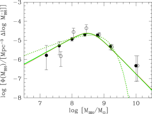
Figure 10.— Binned active BHMFs for broad-line AGNs derived with soft- (filled circles) and hard- (open circles) band samples. Lines indicate corrected BHMF determined using the Maximum likelihood method with four different combinations of functional forms of BHMF and ERDF. Solid lines are for the double-power-law BHMF and dotted lines are for the Schechter BHMF. Thick lines are determined with the log-normal ERDF and thin lines are determined with the Schechter ERDF. Because the difference of the corrected BHMF with the different ERDFs is small, thick and thin lines overlap.

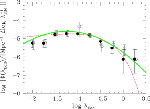
Figure 11.— Binned ERDFs for broad-line AGNs derived with soft- (filled circles) and hard- (open circles) band samples. Lines indicate corrected ERDF determined using the Maximum likelihood method with four different combinations of functional forms of BHMF and ERDF. Solid lines are for the double-power-law BHMF and dotted lines are for the Schechter BHMF. Thick lines are for the log-normal ERDF and thin lines are for the Schechter ERDF. Because the difference of the corrected ERDFs with the different BHMFs is small, solid and dotted lines overlap. All of the ERDFs are normalized by matching the number density in the range $\log\lambda_{\rm Edd}=-2.0-1.0$ to the number density of broad-line AGN BHMF in the range $\log M_{\rm BH}=7.0-11.0$.

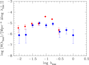
Figure 12.— Binned ERDFs for soft-band broad-line AGNs in the two mass ranges $10^{8.0-8.5}$ and $10^{8.5-9.0}M_{\sun}$ are shown with filled circles and filled diamonds, respectively.

Table 5Binned broad-line AGN BHMF

$\langle\log[M_{\rm BH}/M_{\sun}]\rangle$	$\Phi_{\rm soft}\left(\log M_{\rm BH}\right)$			$N_{\rm soft}$	$\Phi_{\rm{hard}}\left(\log M_{\rm BH}\right)$			$N_{\rm hard}$
7.2	1.65	${}^{+}_{-}$	${}^{3.80}_{1.36}$	1	$\cdots$			0
7.6	5.17	$\pm$	3.41	4	1.50	$\pm$	1.07	2
8.0	11.60	$\pm$	2.43	23	27.46	$\pm$	15.50	17
8.4	19.90	$\pm$	3.55	36	43.21	$\pm$	21.54	30
8.8	18.62	$\pm$	3.36	34	19.93	$\pm$	5.21	28
9.2	4.74	$\pm$	1.50	10	4.53	$\pm$	1.51	9
9.6	$\cdots$			0	$\cdots$			0
10.0	0.47	${}^{+}_{-}$	${}^{1.09}_{0.39}$	1	0.47	${}^{+}_{-}$	${}^{1.09}_{0.39}$	1

Table 6Binned ERDF at $z=1.43$

$\langle\log{\lambda_{\rm Edd}}\rangle$	$\Phi_{\rm soft}\left(\log{\lambda_{\rm{Edd}}}\right)$			$N_{\rm{soft}}$	$\Phi_{\rm hard}\left(\log{\lambda_{\rm{Edd}}}\right)$			$N_{\rm{hard}}$
-2.00	5.79	$\pm$	2.60	6	6.03	$\pm$	3.49	4
-1.75	5.68	$\pm$	2.43	6	6.12	$\pm$	2.89	5
-1.50	16.51	$\pm$	4.11	18	21.29	$\pm$	7.06	14
-1.25	18.36	$\pm$	4.53	20	20.80	$\pm$	7.77	15
-1.00	18.15	$\pm$	4.47	20	46.98	$\pm$	33.71	16
-0.75	15.54	$\pm$	3.77	18	15.23	$\pm$	4.16	15
-0.50	7.12	$\pm$	2.38	10	3.79	$\pm$	1.94	5
-0.25	3.04	$\pm$	1.52	4	4.95	$\pm$	2.28	5
0.00	0.76	${}^{+}_{-}$	${}^{1.75}_{0.63}$	1	2.95	$\pm$	1.76	3
0.25	0.76	${}^{+}_{-}$	${}^{1.74}_{0.63}$	1	0.76	${}^{+}_{-}$	${}^{1.74}_{0.63}$	1

First we derive the binned BHMF and ERDF for the broad-line AGNs between $1.18\leq z\leq 1.68$ using the $V_{\rm max}$ method (Avni & Bahcall, 1980). Detailed numbers for the sample are shown in Table 2. In the calculations of the binned BHMF and ERDF, we only consider broad-line AGNs with $\lambda_{\rm Edd}$ larger than 0.01, and remove 2 broad-line AGNs below the limit. We also remove 2 broad-line AGNs (SXDS0613 and SXDS0738) with neither Mg II nor H${\alpha}$ FWHM measurements in the redshift range. We derive the binned broad-line AGN BHMF and ERDF for the soft- and hard-band samples separately.

For the binned broad-line AGN BHMF, we divide the mass range $6.6\leq\log(M_{\rm BH}/M_{\sun})\leq 10.2$ into 9 bins with bin width, $\Delta\log M_{\rm BH}$, of 0.4 dex. The number density in a bin between $(\log M_{\rm BH}-\Delta\log M_{\rm BH}/2)\sim(\log M_{\rm BH}+\Delta\log M_{\rm BH}/2)$ is given by,

$$\Phi_{\rm BH}(M_{\rm BH})\Delta\log M_{\rm BH}=\sum^{n}_{i=1}\frac{1}{V_{a,i}}.$$ (3)

The summation is done for the $n$ broad-line AGNs in the mass bin. $i$ is the index for a broad-line AGN in the mass bin. $V_{a,i}$ is the effective survey volume for the $i$-th broad-line AGN in the comoving coordinate and its inverse represents the contribution of the broad-line AGN to the comoving number density of the mass bin. $V_{a,i}$ is given by,

$$V_{a,i}=\int^{z_{\rm max}}_{z_{\rm min}}\Omega(L_{{\rm x}i},\log N_{{\rm H}i},z^{\prime})\left(\frac{1+z^{\prime}}{1+z_{\rm cen}}\right)^{k}\frac{{\rm d}V}{{\rm d}z^{\prime}}{\rm d}z^{\prime}.$$ (4)

$z_{\rm min}$ and $z_{\rm max}$ represent the redshift range for the binned broad-line AGN BHMF (1.18 and 1.68, respectively). $\Omega(L_{{\rm X}i},\log N_{{\rm H}i},z^{\prime})$ is the survey area which is calculated assuming that the $i$-th broad-line AGN observed at $z_{i}$ with absorption-corrected luminosity $L_{{\rm X}i}$, absorption hydrogen column density $\log N_{{\rm H}i}$ is at redshift $z^{\prime}$. With an estimated absorption-corrected $L_{{\rm X}i}$ and $\log N_{{\rm H}i}$ as described in Section 2, we calculate the predicted count-rate for each broad-line AGN with $z^{\prime}$ instead of the observed $z_{i}$. The same X-ray spectral model of AGNs is used, as explained in Section 2. The survey area for the sample with likelihood larger than 7 is determined as a function of count-rate for the overlapping region of the X-ray and deep optical surveys (Ueda et al., 2008). The logN-logS relation derived with the area curve for the SXDS X-ray sources is consistent with the relation determined in deeper Chandra surveys (Ueda et al., 2008). The consistency implies the position-dependent detection limit of the X-ray survey is reproduced well in the estimated area curve. If the predicted count-rate of an object at a certain redshift $z^{\prime}$ is below the smallest count-rate limit of the survey, $\Omega(L_{{\rm X}i},\log N_{{\rm H}i},z^{\prime})$ becomes 0 above that redshift. The factor $((1+z^{\prime})/(1+z_{\rm cen}))^{k}$ corrects for the number density evolution with $(1+z)^{k}$ within the redshift range to determine the corresponding number density at $z_{\rm cen}$ of 1.43. However, the correction factor is negligible even if we introduce rather strong number density evolution with $k=4-5$ observed for the X-ray luminosity function of AGNs (Ueda et al., 2003; Hasinger et al., 2005), because the redshift range for this calculation is narrow. Therefore, we neglect this term hereafter and fix the value $k$ as 0 for simplicity. Finally $V_{a,i}$ is obtained by integrating the corresponding survey area for the object at redshift $z^{\prime}$ multiplied by the cosmological volume element $(dV/dz^{\prime})dz^{\prime}$ of unit solid angle in the redshift range. The uncertainty of the binned broad-line AGN BHMF is estimated using Poisson statistics as,

$$\sigma=\left[\sum^{n}_{k=1}\left(\frac{1}{V_{a,i}\ \Delta\log M_{\rm BH}}\right)^{2}\right]^{1/2}.$$ (5)

The resulting binned broad-line AGN BHMFs are shown in Figure 10 and Table 5. The filled and open circles represent the binned BHMFs of soft- and hard-band broad-line AGN samples, respectively. Both of the binned broad-line AGN BHMFs peak at around $M_{\rm BH}$ of $10^{8.5}M_{\sun}$. The binned broad-line AGN BHMFs are consistent each other within the 1 $\sigma$ uncertainty.

The binned broad-line AGN ERDF is derived in the same way for the binned BHMF using the $V_{\rm max}$ method. We bin the sample in $\lambda_{\rm Edd}$ by dividing the $\lambda_{\rm Edd}$ range of $-2.125<\log\lambda_{\rm Edd}<0.375$ into 10 bins with a bin width $\Delta\lambda_{\rm Edd}$ of 0.25 dex. The number density of a certain Eddington ratio bin between ( $\log\lambda_{\rm Edd}-\Delta\log\lambda_{\rm Edd}/2)\sim(\log\lambda_{\rm Edd}+\Delta\log\lambda_{\rm Edd}/2)$ is given by,

$$\Phi_{\lambda}(\lambda_{\rm Edd})\Delta\log\lambda_{\rm Edd} = \sum^{n}_{i=1}\frac{1}{V_{a,i}}.$$ (6)

$n$ is the number of broad-line AGNs in the Eddington ratio bin. $V_{a,i}$ is the same effective volume for the $i$-th broad-line AGN used in the binned BHMF. The uncertainty for each Eddington ratio bin is again given by

$$\sigma = \left[\sum^{n}_{k=1}\left(\frac{1}{V_{a,i}\Delta\log\lambda_{\rm Edd}}\right)^{2}\right]^{1/2}.$$ (7)

The resulting binned ERDF is shown in Figure 11 and tabulated in Table 6. The filled and open circles in the figure are the binned ERDFs for the soft- and hard- band samples, respectively. The binned ERDFs are consistent with each other within the 1 $\sigma$ uncertainty. In the binned ERDFs, broad-line AGNs in the entire mass range are considered. Due to the flux limit of the survey, the sample covers only broad-line AGNs with larger $M_{\rm BH}$ in the lower $\lambda_{\rm Edd}$ bins. Therefore the shape of the binned ERDF can be affected by the flux limit.

In order to examine the $M_{\rm BH}$ dependence of the binned ERDF, in Figure 12, the binned ERDFs derived with the soft-band selected broad-line AGNs in the $M_{\rm BH}$ range between $10^{8.0-8.5}M_{\sun}$ and that between $10^{8.5-9.0}M_{\sun}$ are plotted with filled circles and filled diamonds, respectively. The overall shapes of the binned ERDFs do not significantly differ from each other within the uncertainty, except for the lowest $\log\lambda_{\rm Edd}$ range where the lower mass binned ERDF can be affected by the flux limit. Due to the limited number and mass range of the SXDS sample, there is no signature of the dependence of the ERDF on $M_{\rm BH}$.

5.2. Corrected broad-line AGN BHMF and ERDF with Maximum Likelihood Method

Figure 13.— Effective volume of the SXDS soft-band sample in the redshift range between 1.18 and 1.68 as a function of 2–10 keV hard X-ray luminosity.

Table 7Best fit parameters for the corrected broad-line AGN BHMF and ERDF

BHMF	ERDF	$\phi^{*}$	$\log M^{*}$	$\alpha$	$\beta$	$\log\lambda_{\rm Edd}^{*}$	$\alpha_{\lambda}$	2DKS	Note
DPL	SCH	$19.82_{-3.20}^{+3.20}$	$8.57_{-0.15}^{+0.16}$	$-0.05_{-0.28}^{+0.35}$	$-2.67_{-0.39}^{+0.28}$	$-0.58_{-0.10}^{+0.12}$	$-0.74_{-0.15}^{+0.15}$	86
SCH	SCH	$20.80_{-3.20}^{+3.30}$	$8.77_{-0.08}^{+0.08}$	$-0.35_{-0.14}^{+0.15}$	$\cdots$	$-0.59_{-0.10}^{+0.11}$	$-0.74_{-0.15}^{+0.15}$	65	$\times$
DPL	LOG	$19.39_{-3.20}^{+3.20}$	$8.59_{-0.15}^{+0.16}$	$-0.09_{-0.27}^{+0.34}$	$-2.70_{-0.40}^{+0.29}$	$-2.87_{-0.20}^{+0.16}$	$1.25_{-0.11}^{+0.14}$	79
SCH	LOG	$20.61_{-3.20}^{+3.30}$	$8.78_{-0.08}^{+0.08}$	$-0.35_{-0.14}^{+0.15}$	$\cdots$	$-2.88_{-0.20}^{+0.16}$	$1.24_{-0.10}^{+0.13}$	62

Both the binned broad-line AGN BHMF and ERDF are affected by the detection limit determined by the X-ray count rate; at the low-mass end of the binned BHMF the sample covers only high $\lambda_{\rm Edd}$ broad-line AGNs and at the low Eddington ratio end of the binned ERDF the sample does not include broad-line AGNs with low $M_{\rm BH}$. Such detection limits are not corrected for in the calculations of the binned broad-line AGN BHMF and ERDF.

The effects of the detection limit can be corrected through statistical methods assuming the forms of both functions (Kelly et al., 2009, 2010; Schulze & Wisotzki, 2010; Shen & Kelly, 2012; Kelly & Shen, 2012). Schulze & Wisotzki (2010) apply the Maximum likelihood method to a sample of low-redshift broad-line AGNs detected in the ESO/Hamburg survey, assuming that the intrinsic ERDF does not depend on $M_{\rm BH}$. On the other hand, Kelly et al. (2010), Shen & Kelly (2012) and Kelly & Shen (2012) apply a Bayesian approach (Kelly et al., 2009) to SDSS broad-line AGNs. They introduce a dependence of ERDF on the black hole mass. Furthermore, the statistical scatter in the virial black hole mass estimate is considered in the calculations; the scatter can broaden a peak in the intrinsic broad-line AGN BHMF and a steep slope of intrinsic BHMF at the high-mass end can become flatter in the binned BHMF. If the intrinsic BHMF has a peak at a certain black hole mass and there is a turn-over at the low-mass end, the scatter can also affect the binned BHMF in the low-mass end.

Here, we apply Maximum likelihood method used in Schulze & Wisotzki (2010) for the broad-line AGNs in the soft-band sample. Because there is no significant difference between the binned broad-line AGN ERDFs in the high- and low-mass ranges as shown in Figure 12, we assume that the intrinsic broad-line AGN ERDF is constant regardless of black hole mass. The effect of the scatter of the virial black hole mass estimate is not considered in this paper, because the SXDS sample covers smaller black hole mass and Eddington ratio ranges than the SDSS sample, most of the SXDS broad-line AGNs lie in the mass range below the knee of the BHMF, and in order not to be affected by the uncertainty associated with the modeling of the scatter. The high-mass end of the corrected broad-line AGN BHMF can be affected by the flattening due to the scatter.

In this evaluation, we assume the shape of the corrected broad-line AGN BHMF to be either a double-power-law or a Schechter function,

$$\Phi_{\rm BH}(M_{\rm BH})$$ (9)

$$= \frac{M_{\rm BH}}{\log_{10}e}\frac{\phi^{*}}{M^{*}}\left(\frac{1}{(M_{\rm BH}/M^{*})^{-\alpha}+(M_{\rm BH}/M^{*})^{-\beta}}\right),$$

$$\Phi_{\rm BH}(M_{\rm BH})$$

$$= \frac{M_{\rm BH}}{\log_{10}e}\frac{\phi^{*}}{M^{*}}\left(\frac{M_{\rm BH}}{M^{*}}\right)^{\alpha}\exp\left(-\frac{M_{\rm BH}}{M^{*}}\right),$$

respectively, with the functions expressed per $\log M_{\rm BH}$. We introduce these two forms because the double-power-law describes the AGN luminosity function well, and the Schechter function describes the luminosity and mass functions of galaxies. Even though a modified Schechter function describes the non-active BHMF in the local Universe (Aller & Richstone, 2002; Shankar et al., 2004), we do not implement such a function, since it does not converge and results in a rather small $M^{*}$ ($10^{5-6}M_{\sun}$).

For the corrected ERDF we assume the Schechter function and the log-normal distributions.

$$\Phi_{\lambda}(\lambda_{\rm Edd})$$

$$= \frac{\lambda_{\rm Edd}}{\log_{10}e}\frac{\phi^{*}_{\lambda}}{\lambda_{\rm Edd}^{*}}\left(\frac{\lambda_{\rm Edd}}{\lambda_{\rm Edd}^{*}}\right)^{\alpha_{\lambda}}\exp\left(-\frac{\lambda_{\rm Edd}}{\lambda_{\rm Edd}^{*}}\right),$$

$$\Phi_{\lambda}(\lambda_{\rm Edd})$$

$$= \frac{1}{\lambda_{\rm Edd}\sqrt{2\pi\sigma^{2}}}\exp\left(-\frac{({\rm ln}\lambda_{\rm Edd}-\mu)^{2}}{2\sigma^{2}}\right).$$ (11)

We do not consider the $M_{\rm BH}$ dependence of the ERDF. For both distributions, we define the normalized corrected ERDF with

$$P_{\lambda}(\lambda_{\rm Edd})=\frac{\Phi(\lambda_{\rm Edd})}{\displaystyle\int_{-2.0}^{1.0}\Phi(\lambda_{\rm Edd}){\rm d}\log\lambda_{\rm Edd}}.$$ (12)

We normalize the corrected ERDF in the range $\log\lambda_{\rm Edd}$ of $-2.0$ and $1.0$. In these functions, $\phi^{*}$, $\alpha$, $\beta$, and $M^{*}$ of the corrected BHMF and $\alpha_{\lambda}$ and $\lambda_{\rm Edd}^{*}$ of the corrected ERDF (or $\sigma$ and $\mu$ for log-normal ERDF) are free parameters. We derive the best fit parameters with the Maximum Likelihood method (Marshall et al., 1983). The likelihood function is written as

$$S = -2\sum_{i=1}^{N}{\rm ln}\ p(M_{{\rm BH},i},\lambda_{{\rm Edd},i})$$ (13)

$$+ 2\int\int p(M_{\rm BH},\lambda_{{\rm Edd}})\ d\log\lambda_{\rm Edd}\ d\log M_{\rm BH}$$

and the model parameters that minimize $S$ are the best fit parameters (Marshall et al., 1983). The sum of the first term will be taken for the entire $N$ broad-line AGNs in the sample. The term $p(M_{\rm BH},\lambda_{\rm Edd})$ is the expected number of black holes with $M_{\rm BH}$ and $\lambda_{\rm Edd}$ in unit $\log M_{\rm BH}$ and $\log\lambda_{\rm Edd}$ intervals in the survey redshift range with the assumed $\Phi_{\rm BH}(M_{\rm BH})$ and $P_{\lambda}(\lambda_{\rm Edd})$. $p(M_{\rm BH},\lambda_{\rm Edd})$ is given by

$$p(M_{\rm BH},\lambda_{\rm Edd})$$

$$= \int_{z_{\rm min}}^{z_{\rm max}}\Omega^{\prime}(M_{\rm BH},\lambda_{\rm Edd},z^{\prime})$$

$$P_{\lambda}(\lambda_{\rm Edd})\Phi_{\rm BH}(M_{\rm BH})\left(\frac{1+z^{\prime}}{1+z_{\rm cen}}\right)^{k}\frac{{\rm d}V}{{\rm d}z^{\prime}}{\rm d}z^{\prime}.$$

$\Omega^{\prime}(M_{\rm BH},\lambda_{\rm Edd},z^{\prime})$ is the survey area for an broad-line AGN with $M_{\rm BH}$ and $\lambda_{\rm Edd}$ at $z^{\prime}$. We calculate the expected count rate for each combination of $M_{\rm BH}$, $\lambda_{\rm Edd}$, and $z^{\prime}$ assuming the same model for the X-ray spectrum of AGNs used in Section 2. We convert the $L_{\rm bol}$ for a combination of $M_{\rm BH}$ and $\lambda_{\rm Edd}$ to $L_{\rm 2-10~{}keV}$ with the bolometric correction factor from Marconi et al. (2004). In this calculation we do not consider the effect of X-ray absorption because the effect is not significant for the sample of broad-line AGNs. In Figure 13, we plot the effective volume

$$V_{\rm eff}=\int_{z_{\rm min}}^{z_{\rm max}}\Omega^{\prime}(M_{\rm BH},\lambda_{\rm Edd},z^{\prime})\frac{{\rm d}V}{{\rm d}z^{\prime}}{\rm d}z^{\prime}$$ (15)

as a function of $L_{\rm 2-10~{}keV}$. We consider $\log\lambda_{\rm Edd}$ down to $-2.0$ and $M_{\rm BH}$ of $10^{6}M_{\sun}$. Again we use $k$ of 0 as explained in the previous subsection. We minimize $S$ with the 6 free parameters with the downhill simplex algorithm (Nelder & Mead, 1965). The 1$\sigma$ uncertainty of the best-fit parameters for each model can be evaluated by the increase of $S$ by 1 from the minimum value. In order to determine the 1$\sigma$ uncertainty of each parameter, the parameter is changed from its best value to a different value, and fixing the parameter at the value, the same minimization process is applied for the other parameters and we evaluate the change of the minimum $S$ value from the best fit value of $S$. The uncertainty of the selected parameter is determined by the change of the minimum of 1 from the best fit value. The resulting best-fit parameters are summarized in Table 7.

The resulting corrected broad-line AGN BHMFs and ERDFs are shown in Figures 10 and 11. The corrected ERDFs are normalized by matching the number density in the range $\log\lambda_{\rm Edd}=-2.0-1.0$ and that of the corrected BHMF in the range $\log M_{\rm BH}=7.0-11.0$. The corrected BHMF follows the estimated number density with the $V_{\rm max}$ method well in the mass range above $10^{8.5}M_{\sun}$. This is consistent with the limit of the SXDS sample; it extends down to a Eddington ratio of 0.01 in the mass range above $\sim 10^{8}M_{\sun}$. In the lower mass range, the corrected BHMF is slightly larger than the number density derived with the $V_{\rm max}$ method. The estimated correction is consistent with the corrected ERDF; for 10${}^{7.5}M_{\sun}$ black holes the sample covers a Eddington ratio of $\sim 0.1$, and the ratio below and above this Eddington ratio is $1.7-1.8$ from the corrected ERDF. Therefore, the estimated correction is not large. The shape of the corrected ERDF is consistent with that derived in the $10^{8}-10^{9}M_{\sun}$ mass range with the $V_{\rm max}$ method. The correction required for the ERDF is only significant in the low Eddington range, $\log\lambda_{\rm Edd}$ below $-1.5$. Thanks to the coverage for relatively low-luminosity broad-line AGNs, the SXDS sample is rather complete in a wide mass and Eddington ratio range.

The minimum value of the likelihood function does not reflect the goodness of the fit. We evaluate the goodness of the fit by applying the two-dimensional Kolmogorov-Smirnov (2DKS) test on the distribution of the sample in the $M_{\rm BH}$ and $\lambda_{\rm Edd}$ plane (Fasano & Franceschini, 1987). The resulting 2DKS probability for the deviation in the plane are shown in Table 7. All of them exceed 20% and all of the models fit well the distribution of objects on the plane.

In the mass range below $10^{8.5}$M_☉, the corrected BHMFs show possible decline to the low-mass end. The mass range is well above the detection limit as shown in Figure 9, but the decline can be affected by the completeness of the broad-line AGN sample. For example, there is a possibility that among objects without spectroscopic identification low-luminosity broad-line AGNs whose SEDs are dominated by host galaxy components are classified as narrow-line AGNs in the photometric redshift estimation, and they would be missed in the current broad-line AGN sample.

5.3. Constraint from the Hard X-ray Luminosity Function

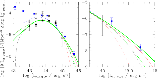
Figure 14.— Left) Hard X-ray luminosity function of X-ray-selected AGNs (Ueda et al. 2012, in preparation; filled squares) compared with that reproduced from the corrected broad-line AGN BHMFs and ERDFs (lines). The open circles and squares show the luminosity function derived from the soft-band-selected and hard-band-selected AGN samples of SXDS in the range $1.18<z<1.68$, respectively. Filled circles represent the luminosity function of broad-line AGNs in the soft-band sample, which is used to derive the corrected broad-line AGN BHMF and ERDF. The hard X-ray luminosities of all AGNs are corrected for intrinsic absorption. Solid and dotted lines correspond to the luminosity functions for the BHMF characterized by double-power-law and Schechter functions and the thick and thin lines are those derived with the Schechter and log-normal ERDF, respectively. The thin dot-dashed line shows the luminosity function derived with double-power-law BHMF $+$ log-normal ERDF with limiting $M_{\rm BH}$ range below $10^{10}M_{\sun}$. The thin long-dashed line represents the luminosity function with double-power-law BHMF $+$ log-normal ERDF after correcting for the obscured fraction following Hasinger (2008). Right) Zoom in version of the left panel in the high-luminosity range.

The luminosity function of broad-line AGNs is the convolution of their BHMF and ERDF, therefore we can constrain the shapes of broad-line AGN BHMF and ERDF further by using the luminosity function determined from a combination of various AGN samples. In particular, the number density at the bright end of the luminosity function obtained through wider but shallower surveys than SXDS can constrain the shapes of broad-line AGN BHMF and ERDF in the high $M_{\rm BH}$ and $\lambda_{\rm Edd}$ range. It needs to be noted that the fraction of obscured narrow-line AGNs is low in the luminosity range (Hasinger, 2008) and the luminous end of the luminosity function is thought to be dominated by broad-line AGNs.

In Figure 14, we plot the observed hard X-ray luminosity function of AGNs at $z=1.2-1.6$ based on a combined sample of AGNs from various hard X-ray surveys as filled squares (Ueda et al. 2012, in preparation). The horizontal axis is the absorption-corrected 2–10 keV luminosity. The hard X-ray luminosity functions of the broad-line + narrow-line AGNs in the SXDS soft-band-selected and hard-band-selected samples are shown as open circles and squares, respectively. The hard-band-selected AGN luminosity function in the SXDS is consistent with that derived from the combined sample. The soft-band-selected AGN luminosity function has slightly lower number density than the hard-band-selected AGN luminosity function below $L_{\rm 2-10~{}keV}=10^{44}$ erg s^-1. The lower number density can be qualitatively explained with the fact that the soft-band-selected sample misses heavily obscured AGNs and the fraction of obscured AGNs is larger for AGNs with lower luminosity. Because all of the luminosity functions are consistent each other in the luminosity range above $L_{\rm 2-10~{}keV}=10^{44}$ erg s^-1, therefore we use the number density of AGNs at the luminous end of the combined sample as the constraint on the broad-line AGN BHMF and ERDF.

The filled circles represent the hard X-ray luminosity function of broad-line AGNs in the soft-band samples. Again the hard X-ray luminosity is corrected for intrinsic absorption. The hard X-ray luminosity function shows turn over at $L_{\rm 2-10~{}keV}=10^{44}$ (erg s^-1). Such turn over is also observed in the broad-line AGN hard X-ray luminosity function at $z=1-3$ from Chandra surveys (Yencho et al., 2009). At least part of the decrease can be explained with the increasing fraction of obscured narrow-line AGNs in the lower luminosity range as described below. The lines in the figure show the hard X-ray luminosity function derived from the convolution of the corrected broad-line BHMF and ERDF. Solid and dotted lines correspond to luminosity functions with the corrected BHMF of double-power-law and Schechter forms and the thick and thin lines are those derived with Schechter and log-normal ERDF, respectively. The hard X-ray luminosity for each set of $M_{\rm BH}$ and $\lambda_{\rm Edd}$ is derived with the bolometric correction for 3000Å monochromatic luminosity and the relation between $\lambda 3000L_{\lambda 3000}$ and $L_{\rm 2-10keV}$ shown with the solid line in Figure 7. Considering the upper limit of the observed $M_{\rm BH}$ of broad-line AGNs (Vestergaard et al., 2008) and local galaxies (McConnell et al., 2011), we limit the $M_{\rm BH}$ range to be $10^{6-10.5}M_{\sun}$ and the $\log\lambda_{\rm Edd}$ range to be $-2$ and $1$.

The hard X-ray luminosity functions derived with the double-power-law BHMF or log-normal ERDF can reproduce the observed number density at the high-luminosity end. On the contrary, if both the BHMF and ERDF are modeled with an exponential-cutoff such as the Schechter BHMF with Schechter ERDF (thin dotted line), the high-luminosity end of the luminosity function cannot be reproduced; the predicted number density is more than one order of magnitude smaller than the observed luminosity function. Therefore such models are unlikely to represent the BHMF and ERDF of broad-line AGNs at $z=1.4$. Furthermore, if we limit the mass range of BHMF up to $10^{10}M_{\sun}$, the predicted luminosity function with a double-power-law BHMF and log-normal ERDF are represented by the dot-dashed line in the figure; the predicted density in the high luminosity end is much lower than the observed one. Thus in order to reproduce the number density of luminous AGNs, the BHMF needs to be extended up to $10^{10.5}M_{\sun}$ under the assumption that the ERDF is constant over the wide $M_{\rm BH}$ range.

In the luminosity range below $L_{\rm 2-10~{}keV}=10^{44}$ erg s^-1, the broad-line AGN luminosity function shows decline toward lower luminosity. At least part of the decline can be explained with the increasing fraction of obscured narrow-line AGNs in the lower luminosity range. In Figure 14, we also plot model luminosity function derived with a double-power-law BHMF and log-normal ERDF after correcting the fraction of narrow-line AGN following Hasinger (2008) with thin long dashed line. In Hasinger (2008), luminosity dependence of the fraction is derived as a function of redshift. We use the relation derived at $z=1.2-1.6$. Although the corrected luminosity function still has lower number density than the broad-line $+$ narrow-line AGN luminosity function, the large fraction of the discrepancy between the broad-line luminosity function and total luminosity function seems to be explained with the obscured fraction down to $L_{\rm 2-10~{}keV}=10^{43}$ erg s^-1. The remaining discrepancy can be caused by the possible incompleteness of the broad-line AGN BHMF due to the spectroscopic incompleteness and the difficulties in identifying broad-line AGNs with substantial host contamination. The uncertainty of the fraction of narrow-line AGN is still large and the sample size of the SXDS is limited. Larger sample is necessary to understand the remaining discrepancy.

6. Discussion

6.1. Broad-line AGN BHMF at z $\sim$1.4 and Its evolution to $z=0$

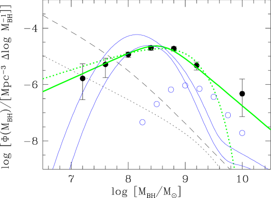
Figure 15.— Binned (filled circles) and corrected broad-line AGN BHMFs (thick solid line with double-power-law model and thick dashed line with Schechter model) from SXDS compared with binned (open circles) and estimated (thin solid lines) broad-line AGN BHMFs at $z\sim 1.4$ from SDSS (Shen & Kelly, 2012). Upper and lower thin solid lines enclose the 68% possible area. The thin dashed line shows the corrected broad-line AGN BHMF in the local Universe from Schulze & Wisotzki (2010). The thin dotted line indicates the total BHMF at $z=6$ from Willott et al. (2010).

The binned and corrected broad-line AGN BHMFs from the soft-band sample are compared with the binned and estimated broad-line AGN BHMF from the SDSS sample (Shen & Kelly, 2012) in Figure 15. The SXDS binned BHMFs (filled circles) is larger than the binned BHMF of the SDSS sample (open circles) by 1 order of magnitude at $10^{8.5}M_{\sun}$, and by two orders of magnitude at $10^{8}M_{\sun}$. This is mostly because broad-line AGNs with lower Eddington ratio are detected in the SXDS sample than in the SDSS; the SDSS sample is only 30% complete down to $M_{\rm BH}$ of $\sim 10^{9}M_{\sun}$ and $\lambda_{\rm Edd}$ of $\sim 0.6$ at $z=1.4$ (Kelly et al., 2010). Additionally, as discussed in Section 3.4, the SXDS sample covers even mildly obscured broad-line AGNs that may be missed in the SDSS selection of broad-line AGNs due to color and stellarity issues. The thin solid lines in the figure represent the upper and lower envelopes of the estimated broad-line AGN BHMF with a Bayesian approach (Shen & Kelly, 2012). The estimated number density at $10^{8}M_{\sun}$ is consistent with the binned and corrected BHMF of SXDS.

We examine the evolution of broad-line AGN BHMF from $z=1.4$ to $0$ by comparing the $z\sim 1.4$ corrected BHMF with that in the local Universe. The dashed lines in the figure show the corrected local ( $z<0.3$ ) broad-line AGN BHMF from Schulze & Wisotzki (2010). The binned BHMFs of broad-line AGNs in the local Universe of Greene & Ho (2009) and Vestergaard & Osmer (2009) are consistent with the binned BHMF of Schulze & Wisotzki (2010). The corrected BHMF at $z\sim 1.4$ exceeds that of local Universe in the mass range above $10^{8}M_{\sun}$. However the behavior in the lower mass range is different; the local broad-line AGN BHMF from Schulze & Wisotzki (2010) shows a steep increase with decreasing black hole mass even below $10^{7}M_{\sun}$ mass range. On the contrary, the SXDS sample shows a hint of turn-over at a mass of $10^{8.5}M_{\sun}$. The difference in the corrected broad-line AGN BHMF may be indicative of a down-sizing trend of accretion activity among the SMBH population. As mentioned in Section 5.2, it needs to be noted that the identification of broad-line AGNs could be incomplete in the low-mass end.

It is also possible that decline of the activity in the low-mass range from $z=0$ to $1.4$ is caused by luminosity and redshift dependent obscuration to the nucleus. Although broad-line AGNs have a wide range of $\lambda_{\rm Edd}$, the fraction of broad-line AGNs with low-mass SMBH is higher in the lower luminosity range. A luminosity dependence of the obscured fraction is observed in various AGN samples (e.g. Akiyama et al., 2000; Ueda et al., 2003; Simpson, 2005; Brusa et al., 2010); the obscured fraction is higher among lower luminosity AGNs. Recently, based on large samples of X-ray selected AGNs, it has also been suggested that the fraction of obscured AGNs is higher at higher redshifts (e.g. Hasinger, 2008; Hiroi et al., 2012). Such redshift and luminosity dependent obscuration may hide activity among low-mass SMBHs at high-redshifts. We examine the contribution from obscured narrow-line AGNs to the total active BHMF in Section 6.4.

6.2. Comparison with total BHMF at z $\sim$6

In order to examine the growth of SMBHs at higher redshift, we compare binned and corrected broad-line AGN BHMF at $z=1.4$ with that at $z=6$. Willott et al. (2010) examined the total BHMF at $z\sim 6$ using the optical luminosity function of broad-line AGNs at that redshift. They derive the total BHMF from the luminosity function using an Eddington ratio distribution derived from a part of their sample. They estimate the total (active + non-active) BHMF by crudely correcting the obscured fraction and duty cycle (active fraction). The resulting best-estimate total BHMF is shown with the thin dotted line in Figure 15. They argue the total BHMF is constrained down to $10^{8}M_{\sun}$. At that mass, the $z=6$ BHMF has a density of $2.5\times 10^{-7}$ Mpc^-3. The number density matches the number density of $z=1.4$ corrected BHMF of broad-line AGNs at $10^{9.5}M_{\sun}$. If we naively assume that the $10^{8}M_{\sun}$ black holes at $z=6$ grow to the $10^{9.5}M_{\sun}$ black holes at $z=1.4$ through accretion, then this implies mass growth by a factor 30 between $z=6$ and $1.4$, i.e., in 3.5 Gyr period. Such growth implies that the multiple of the Eddington ratio and duty cycle has order of 0.1 in that period for the massive SMBHs, if we use the rest mass energy to radiation energy conversion efficiency of 0.1. It needs to be noted that the high-mass end of the corrected BHMF can be affected by the flattening due to the uncertainties of the virial black hole mass estimates, therefore the effect needs to be corrected before further quantitative evaluation of the growth of SMBHs between $z=6$ to $1.4$.

6.3. Eddington Ratio Distribution Functions

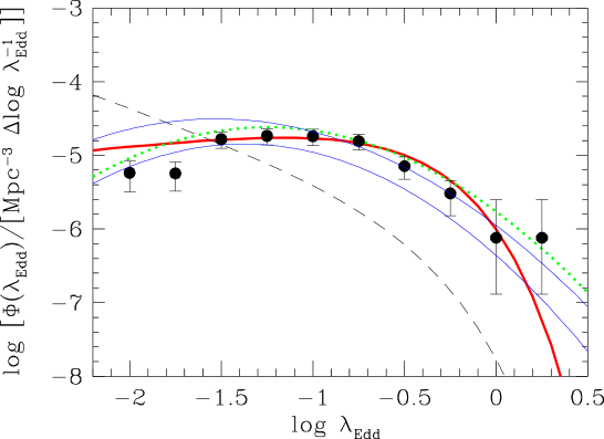
Figure 16.— Binned (filled circles) and corrected broad-line AGN ERDF (thick solid line with Schecheter ERDF and thick dotted line with log-normal ERDF) from SXDS compared with the estimated broad-line AGN ERDF at $z\sim 1.4$ from SDSS (Shen & Kelly, 2012) (thin solid lines). The upper and lower thin solid lines represent the 68% enclosed region. The thin dashed line shows the corrected broad-line AGN ERDF in the local Universe from Schulze & Wisotzki (2010).

Both of the binned and corrected broad-line AGN ERDF show a decline at Eddington ratio of 1. Such a distribution suggests that the accretion of X-ray-selected broad-line AGNs is limited by the Eddington luminosity. In Figure 16, we compare the corrected broad-line AGN ERDF with the estimated broad-line AGN ERDF at $z\sim 1.4$ from the SDSS sample (thin solid lines, Shen & Kelly 2012). The shapes of the ERDFs match rather well. It needs to be noted that there is a possibility that we miss broad-line AGNs accreting at a rate close to the Eddington limit because our X-ray selection is in relatively high energy range; the energy range of the soft-band sample corresponds to 1.2–4.8 keV at $z=1.4$. Optical to X-ray SED models of broad-line AGNs predict weak X-ray emission with steep X-ray spectrum among broad-line AGNs accreting with close to the Eddington limit (Kawaguchi et al., 2001; Done et al., 2012).

In the same figure, we also plot the corrected broad-line AGN ERDF in the local Universe from Schulze & Wisotzki (2010). The shape of their binned ERDF in the local universe is consistent with that derived by Kauffmann & Heckman (2009) for a narrow-line AGN sample from SDSS. The shape of the corrected ERDF in the local Universe has a knee at a similar Eddington ratio ($\log\lambda_{\rm Edd}$ of $-0.6$; Schulze & Wisotzki 2010) to that of the corrected ERDF at $z=1.4$, but shows a steeper increase in the low Eddington ratio range down to $\log\lambda_{\rm Edd}$ of $-2.0$. The evolution of the corrected broad-line AGN ERDF from $z=1.4$ to $0$ indicates the fraction of broad-line AGNs with $\lambda_{\rm Edd}$ close to 1 is higher at higher redshifts.

6.4. Contribution from Obscured Narrow-line AGNs

Figure 17.— Bolometric luminosity versus Eddington ratio of SXDS broad-line AGNs (filled circles). The solid line represents the least square fitting result for the SXDS AGNs. The distribution of SDSS DR5 broad-line AGNs whose $M_{\rm BH}$ is estimated from Mg II (Shen et al., 2008a) is shown by the contours. Crosses represent broad-line AGNs from LBQS (Vestergaard & Osmer, 2009).

Figure 18.— Binned active BHMF with (open triangles) and without (open circles) obscured narrow-line AGNs derived from the hard-band sample. Solid, dotted, and dashed lines indicate the non-active BHMFs at $z=0$, $1$, and $2$ derived with the $K$-band galaxy luminosity functions from Li et al. (2011).

Table 8Binned active BHMF including Obscured Narrow-line AGNs

$\langle\log[M_{\rm BH}/M_{\sun}]\rangle$	$\Phi_{\rm hard}(\log M_{\rm BH})$			$N_{\rm hard}$
7.2	$\cdots$			0
7.6	1.50	$\pm$	1.07	2
8.0	60.95	$\pm$	36.90	18
8.4	139.20	$\pm$	31.42	87
8.8	48.81	$\pm$	7.08	73
9.2	5.06	$\pm$	1.60	10
9.6	$\cdots$			0
10.0	0.47	${}^{+}_{-}$	${}^{1.09}_{0.40}$	1

Among the X-ray-selected AGNs in the redshift range, more than half of the AGNs are obscured narrow-line AGNs as shown in Table 2. In this subsection, the contribution of these obscured narrow-line AGNs to the binned active BHMF is evaluated using the hard-band sample which is less biased against obscured AGNs than the soft-band sample. In the calculation of the binned active BHMF, not only spectroscopically-identified narrow-line AGNs but also narrow-line AGNs with a photometric redshift are included. Because we use the sample of the hard X-ray selected AGNs, the contribution from the heavily-obscured Compton-thick AGNs are not included. The black hole mass of the obscured narrow-line AGNs cannot be estimated from the FWHM of broad-line. Here, their black hole mass is estimated assuming they have same $\lambda_{\rm Edd}$ as broad-line AGNs with the same bolometric luminosity.

First, the relation between the Eddington ratio and the bolometric luminosity is determined for the broad-line AGNs in the SXDS sample. The $L_{\rm bol}$ vs. $\lambda_{\rm Edd}$ distribution of the broad-line AGNs is shown in Figure 17. There is a correlation between the Eddington ratio and the bolometric luminosity. The solid line in the figure represents the relation determined with the least square fitting,

$$\log\lambda_{\rm Edd}=0.469\times\log L_{\rm bol}-22.46.$$ (16)

The relation is mainly driven by the virial black hole mass estimator used, and the scatter reflects the distribution of the FWHM. The scatter of the $\lambda_{\rm Edd}$ from the best fit relation is 0.4 dex, which is roughly consistent with the width of the distribution of the FWHM. In the figure, the distribution of SDSS (Shen et al., 2008a) and Large Bright Quasar Survey (LBQS) (Vestergaard & Osmer, 2009) broad-line AGNs are also shown with the contours and crosses. For the SDSS sample, only broad-line AGNs with $M_{\rm BH}$ from Mg II measurements are shown. All of the broad-line AGNs follow the same trend of increasing $\log\lambda_{\rm Edd}$ with increasing $L_{\rm Bol}$ as discussed in Croom (2011).

For obscured narrow-line AGNs, their bolometric luminosities are estimated from the absorption corrected 2–10 keV luminosity with a bolometric correction factor for the 2–10 keV luminosity (Marconi et al., 2004). We do not use UV or optical luminosities to estimate bolometric luminosity, because they are severely suffered from dust extinction and contamination from host galaxies. Using the above Eddington ratios for three bolometric luminosity bins, we estimate black hole mass of each narrow-line AGNs as

$$M_{\rm BH}[M_{\sun}]=\frac{L_{\rm bol}[{\rm erg\ s^{-1}}]}{1.26\times 10^{38}\times\lambda_{\rm Edd,median}}.$$ (17)

The scatter of the $L_{\rm bol}$ and $\lambda_{\rm Edd}$ relation is large, thus the black hole mass estimation is only valid in statistical sense. The binned BHMF derived including the narrow-line AGNs is shown in Figure 18 and is tabulated in Table 8. The contribution of the obscured narrow-line AGNs is large in the mass range, $\log M_{\rm BH}\leq 8.5$.

In order to examine the fraction of active black holes in the entire SMBH population, we compare the binned active BHMF including narrow-line AGNs with non-active BHMF at intermediate redshifts derived from the galaxy luminosity functions and $M_{\rm BH}$ vs. $L_{\rm bulge}$ relationship (Tamura et al., 2006; Li et al., 2011). Li et al. (2011) estimate the non-active BHMF up to $z\sim 2$ from the galaxy $K$-band luminosity function, stellar mass function, and their redshift evolution. They assume an evolution of the $M_{\rm BH}$ vs. $L_{\rm bulge}$ relationship as a function of redshift of the form $M_{\rm BH}/L_{\rm spheroid,K}\propto(1+z)^{1.4}$ following Bennert et al. (2010). They also consider the redshift evolution of the average bulge-to-total luminosity ratio, even though they do not include luminosity dependence of the ratio. The resulting non-active BHMF is consistent with that estimated in the local Universe (Vika et al., 2009). In the figure, the estimated non-active BHMFs at $z=0$, $1$, and $2$ from Li et al. (2011) are plotted with the solid line, dashed line, and dotted line, respectively. The binned active BHMF including narrow-line AGNs lies between the non-active BHMFs at $z=1$ and $2$ in the mass range above $M_{\rm BH}=10^{8.5}M_{\sun}$; a rather high fraction of active SMBHs in the mass range is implied at $z=1.4$. It needs to be noted that the binned active BHMF is not corrected for the scatter of the virial black hole mass estimate and that of the relation between the $\log L_{\rm bol}$ and the $\log\lambda_{\rm Edd}$. Therefore, the number density can be overestimated in the high-mass end due to the contamination from the objects in the lower mass range. In order to discuss the fraction of active SMBHs quantitatively, the scatters needs to be corrected.

7. Summary

Black hole masses of X-ray-selected broad-line AGNs detected in the SXDS are estimated from the width of the Mg II broad-line and the 3000Å monochromatic luminosity. Because optical spectroscopic observations covering the Mg II wavelength range are not complete for the entire X-ray-selected broad-line AGNs, the width of H$\alpha$ broad-line measured with NIR spectroscopic survey is also used to provide a supplementary estimate if black hole masses for broad-line AGNs whose Mg II broad-line width is not available. The sample of broad-line AGNs is selected using X-ray detection as well as detection of a broad emission line of either Mg II in the optical or H$\alpha$ in the NIR. Some of the broad-line AGNs have red rest-frame UV-colors, suggesting mild obscuration to their nucleus. For such broad-line AGNs, the hard X-ray luminosity is used to estimate their intrinsic 3000Å monochromatic luminosity assuming typical optical to X-ray luminosity ratio as a function of bolometric luminosity. In total, black hole masses are estimated for 215 broad-line AGNs at redshifts between 0.5 and 2.3. In the redshift range between 1.18 and 1.68, the black hole mass estimate is highly complete thanks to the supplemental measurements of the H$\alpha$ line width from the NIR spectra.

Using the black hole masses of broad-line AGNs in the redshift range, binned broad-line AGN BHMF and ERDF are initially calculated using the $V_{\rm max}$ method. The binned BHMF shows a peak at $10^{8.5}M_{\sun}$. The binned ERDF has a steep decline at $\lambda_{\rm Edd}$ of 1 and a rather flat distribution below the Eddington limit. Because the sample is X-ray-flux limited, both the binned BHMF and ERDF are affected by the detection limit; the low $M_{\rm BH}$ end of the binned BHMF misses the low $\lambda_{\rm Edd}$ objects and the low $\lambda_{\rm Edd}$ end of the binned ERDF does not include the low $M_{\rm BH}$ broad-line AGNs. The effect of the flux limit is corrected by assuming that the ERDF is constant regardless of the black hole mass. Applying the Maximum Likelihood method with appropriate functional shapes for the broad-line AGN BHMF and ERDF, we determine the corrected BHMF and ERDF. We do not correct for the effect of the uncertainties in the virial black hole mass estimates. Thanks to the faint detection limit, the sample extends down to $\lambda_{\rm Edd}$ of 0.01 in the redshift range, the correction is rather small and the shapes of the corrected BHMF and ERDF do not significantly differ from those of binned BHMF and ERDF.

The corrected broad-line AGN BHMF peaks at $10^{8.5}M_{\sun}$ and shows a possible decline at the low-mass end. The number density around $10^{8}M_{\sun}$ is consistent with that estimated from the SDSS sample. The shape of the corrected BHMF is completely different to that in the local Universe which shows a steep increase down to $10^{7}M_{\sun}$. The evolution of the shape of the corrected BHMF of broad-line AGNs from $z=1.4$ to $z=0$ may be indicative of a down-sizing trend of accretion activity among the SMBH population.

The corrected broad-line AGN ERDF also shows a strong decline at the Eddington-limit and rather flat distribution below the limit. The shape is also consistent with that estimated from the SDSS sample. The strong decline suggests that the accretion of X-ray-selected broad-line AGNs is limited by the Eddington luminosity. The shape of the corrected ERDF in the local Universe has a knee at a similar Eddington ratio but shows a steeper increase in the low Eddington ratio range down to $\lambda_{\rm Edd}$ of 0.01. The evolution of the ERDF from $z=1.4$ to $z=0$ indicates the fraction of broad-line AGNs with $\lambda_{\rm Edd}$ close to 1 is higher at higher redshifts.

Using the hard-band sample of X-ray-selected AGNs, we evaluate the contribution of obscured narrow-line AGNs to the binned active BHMF. We estimate the black hole masses of narrow-line AGNs assuming the same Eddington ratio as a function of bolometric luminosity as for broad-line AGNs. Once the contribution from narrow-line AGNs is included, the binned active BHMF shows a comparable number density to the non-active BHMFs at $z=1-2$ above $M_{\rm BH}$ of $10^{8.5}M_{\sun}$. Such a high density of active SMBHs at $z=1.4$ suggests that massive SMBHs have high active fraction in the redshift range.

References

- Aird et al. (2010) Aird, J., Nandra, K., Laird, E. S., et al., 2010, MNRAS, 401, 2531
- Akiyama et al. (2000) Akiyama, M., Ohta, K., Yamada, T., et al., 2000, ApJ, 532, 700
- Akritas & Bershady (1996) Akritas, M. G., & Bershady, M. A., 1996, ApJ, 470, 706
- Aller & Richstone (2002) Aller, M. C., & Richstone, D., 2002, ApJ, 124, 3035
- Assef et al. (2011) Assef, R. J., Kochanek, C. S., Ashby, M. K. N., et al., 2011, ApJ, 728, 56
- Avni & Bahcall (1980) Avni, Y., & Bahcall, J.N., 1980, ApJ, 235, 694
- Bennert et al. (2010) Bennert, V. N., Treu, T., Woo, J.-H., Malkan, M. A., & Bris, A. L., 2010, ApJ, 708, 1507
- Bentz et al. (2006) Bentz, M. C., Peterson, B. M., Pogge, R. W., Vestergaard, M., & Onken, C. A., 2006, ApJ, 644, 133
- Bolzonella et al. (2000) Bolzonella, M., Miralles, J.-M., & Pello, R., 2000, A&A, 363, 476
- Boyle & Terlevich (1998) Boyle, B. J., & Terlevich, R. J., 1998, MNRAS, 293, L49
- Brammer et al. (2008) Brammer, G. B., van Dokkum, P. G., Coppi, P., 2008, ApJ, 686, 1503
- Brusa et al. (2010) Brusa, M., Civano, F., Comastri, A., et al., 2010, ApJ, 716, 348
- Cardamone et al. (2010) Cardamone, C. N., van Dokkum, P. G., Urry, C. M., et al., 2010, ApJS, 189, 270
- Cowie et al. (2002) Cowie, L. L., Garmire, G. P., Bautz, M. W., et al., 2002, ApJ., 566, L5
- Cristiani et al. (1996) Cristiani, S., Trentini, S., La Franca, F., et al., 1996, A&A, 306, 395
- Croom et al. (2009) Croom, S. M., Richards, G. T., Shanks, T., et al., 2009, MNRAS, 399, 1755
- Croom (2011) Croom, S. M., 2011, ApJ, 736, 161
- Done et al. (2012) Done, C., Davis, S. W., Jin, C., Blaes, O., & Ward, M., 2012, MNRAS, 420, 1848
- Fasano & Franceschini (1987) Fasano, G., & Franceschini, A., 1987, MNRAS, 225, 155
- Furusawa et al. (2008) Furusawa, H., Kosugi, G., Akiyama, M., et al. 2008, ApJS, 176, 1
- Gehrels (1986) Gehrels, N., 1986, ApJ, 303, 336
- Graham et al. (2011) Graham, A. W., Onken, C. A., Athanassoula, E., & Combes, F., 2011, MNRAS, 412, 2211
- Greene & Ho (2005) Greene, J.E., & Ho, L.C., 2005, ApJ, 630, 122
- Greene & Ho (2007) Greene, J.E., & Ho, L.C., 2007, ApJ, 667, 131
- Greene & Ho (2009) Greene, J.E., & Ho, L.C., 2009, ApJ, 704, 1743
- Greene et al. (2010a) Greene, J.E., Hood, C.E., Barth, A.J., et al., 2010a, ApJ, 723, 409
- Greene et al. (2010b) Greene, J.E., Peng, C.Y., & Ludwig, R.R., 2010b, ApJ, 709, 937
- Gültekin et al. (2009) Gültekin, K., Cackett, E. M., Miller, J. M., et al., 2009, ApJ, 698, 198
- Hao et al. (2005) Hao, L., Strauss, M. A., Tremonti, C. A., et al., 2005, ApJ, 129, 1783
- Hasinger et al. (2005) Hasinger, G., Miyaji, T., & Schmidt, M., 2005, A&A, 441, 417
- Hasinger (2008) Hasinger, G., 2008, A&A, 490, 905
- Hiroi et al. (2012) Hiroi, K., Ueda, Y., Akiyama, M., & Watson, M., 2012, ApJ, submitted
- Iwamuro et al. (2012) Iwamuro, F., Moritani, Y., Yabe, K., et al., 2012, PASJ, 64, 59
- Kaspi et al. (2000) Kaspi, S., Smith, P. S., Netzer, H., et al., 2000, ApJ, 533, 631
- Kaspi et al. (2005) Kaspi, S., Maoz, D., Netzer, H., et al., 2005, ApJ, 629, 61
- Kauffmann & Heckman (2009) Kauffmann, G., & Heckman, T., 2009, MNRAS, 397, 135
- Kawaguchi et al. (2001) Kawaguchi, T., Shimura, T., & Mineshige, S., 2001, ApJ, 546, 966
- Kelly et al. (2009) Kelly, B. C., Vestergaard, M., & Fan, X., 2009, ApJ, 692, 1388
- Kelly et al. (2010) Kelly, B. C., Vestergaard, M., Fan, X., et al., 2010, ApJ, 719, 1315
- Kelly & Shen (2012) Kelly, B. C., & Shen, Y., 2012, submitted to ApJ, arXiv:1209.0477
- Kimura et al. (2010) Kimura, M., Maihara, T., Iwamuro, F., et al., 2010, PASJ, 62, 1135
- Korista et al. (1997) Korista, K., Baldwin, J., Ferland, G., & Verner, D., 1997, ApJS, 108, 401
- Kormendy & Richstone (1995) Kormendy, J., & Richstone, D., 1995, ARA&A, 33, 581
- Li et al. (2011) Li, Y-R., Ho, L. C., & Wang, J-M., 2011, ApJ, 742, 33
- Luo et al. (2010) Luo, B., Brandt, W. N., Xue, Y. Q., et al., 2010, ApJS, 187, 560
- Magdziarz & Zdziarski (1995) Magdziarz, P., & Zdziarski, A. A. 1995, MNRAS, 273, 837
- Magorrian et al. (1998) Magorrian, J., Tremaine, S., Richstone, D., et al., 1998, ApJ, 115, 2285
- Marconi & Hunt (2003) Marconi, A., & Hunt, L.K., 2003, ApJ, 589, L21
- Marconi et al. (2004) Marconi, A., Risaliti, G., Gilli, R., et al., 2004, MNRAS, 351, 169
- Marconi et al. (2008) Marconi, A., Axon, D. J., Maiolino, R., Nagao, T., & Pastorini, G., 2008, ApJ, 678, 693
- Markwardt (2009) Markwardt, C. B., 2009, Astronomical Data Analysis Software and Systems XVIII ASP Conference Series, 411, 251
- Marshall et al. (1983) Marshall, H.L., Avni, Y., Tananbaum, H., & Zamorani, G., 1983, ApJ, 269, 35
- McConnell et al. (2011) McConnell, N. J., Ma, C-.P., Gebhardt, K., et al., 2011, Nature, 480, 215
- McGill et al. (2008) McGill, K.L., Woo, J-K., Treu, T., & Malkan, M.A., 2008, ApJ, 673, 703
- McLure & Jarvis (2002) McLure, R.J., & Jarvis, M.J., 2002, MNRAS, 337, 109
- McLure & Dunlop (2004) McLure, R.J., & Dunlop, J.S., 2004, MNRAS, 352, 1390
- Nelder & Mead (1965) Nelder, J. A., & Mead, R. A. 1965, Computer J., 7, 308
- Oke (1974) Oke, J.B. 1974, ApJS, 27, 210
- Onken et al. (2004) Onken, C. A., Ferrarese, L., Merritt, D., et al., 2004, ApJ, 615, 645
- Onken & Kollmeier (2008) Onken, C.A., & Kollmeier, J.A., 2008, ApJ, 689, L13
- Park et al. (2012) Park, D., Woo, J-H., Treu, T., et al., 2012, ApJ, 747, 30
- Peterson & Wandel (1999) Peterson, B. M., & Wandel, A., 1999, ApJ, 521, L95
- Peterson et al. (2004) Peterson, B. M., Ferrarese, L., Gilbert, K. M., et al., 2004, ApJ, 613, 682
- Rafiee & Hall (2011) Rafiee, A., & Hall, P.B., 2011, ApJS, 194, 42
- Richards et al. (2003) Richards, G. T., Hall, P. B., Vanden Berk, D. E., et al., 2003, AJ, 126, 1131
- Richards et al. (2006) Richards, G. T., Lacy, M., Storrie-Lombardi, L. J., et al., 2006, ApJS, 166, 470
- Schulze & Wisotzki (2010) Schulze, A., & Wisotzki, L., 2010, A&A, 516, A87
- Shankar et al. (2004) Shankar, F., Salucci, P., Granato, G.L., De Zotti, G., & Danese, L., 2004, MNRAS, 354, 1020
- Shankar et al. (2009) Shankar, F., Weinberg, D. H., & Miralda-Escude, J., 2009, ApJ, 690, 20
- Shen et al. (2008a) Shen, Y., Greene, E., Strauss, M. A., Richards, G. T., & Schneider, D. P., 2008, ApJ, 680, 169
- Shen et al. (2008b) Shen , J., vanden Berk, D. E., Schneider, D. P., & Hall, P. B., 2008, AJ, 135, 928
- Shen et al. (2011) Shen, Y., Richards, G.T., Strauss, M.A., et al., 2011, ApJS, 194, 45
- Shen & Kelly (2012) Shen, Y., & Kelly, B.C., 2012, ApJ, 746, 169
- Shen & Liu (2012) Shen, Y., & Liu, X., 2012, ApJ, 753, 125
- Silverman et al. (2008) Silverman, J. D., Green, P. J., Barkhouse, W. A., et al., 2008, ApJ, 679, 118
- Simpson (2005) Simpson, C., 2005, MNRAS, 360, 565
- Simpson et al. (2012) Simpson, C., Rawlings, S., Ivison, R., et al., 2012, MNRAS, 421, 3060
- Soltan (1982) Soltan, A., 1982, MNRAS, 200, 115
- Stern & Laor (2012) Stern, J., & Laor, A., 2012, MNRAS, 423, 600
- Tamura et al. (2006) Tamura, N., Ohta, K., & Ueda, Y., 2006, MNRAS, 365, 134
- Tsuzuki et al. (2006) Tsuzuki,Y., Kawara, K., Yoshii, Y., et al., 2006, ApJ, 650, 57
- Ueda et al. (2003) Ueda, Y., Akiyama, M., Ohta, K., & Miyaji, T., 2003, ApJ, 598, 886
- Ueda et al. (2008) Ueda, Y., Watson, M.G., Stewart, I.M., Akiyama, M., & Schwope, A.D. 2008, ApJS, 179, 124
- Vestergaard & Wilkes (2001) Vestergaard, M., & Wilkes, B. J., 2001, ApJS, 134, 1
- Vestergaard (2002) Vestergaard, M., 2002, ApJ, 571, 733
- Vestergaard & Peterson (2006) Vestergaard, M., & Peterson, B. M., 2006, ApJ, 641, 689
- Vestergaard et al. (2008) Vestergaard, M., Fan, X., Tremonti, C. A., Osmer, P. S., & Richards, G. T., 2008, ApJ, 674, L1
- Vestergaard & Osmer (2009) Vestergaard, M., & Osmer, P. S., 2009, ApJ, 699, 800
- Vestergaard et al. (2011) Vestergaard, M., Denney, K., Fan, X., Jensen, J. J., Kelly, B. C., Osmer, P. S., Peterson, B. M., & Tremonti, C. A., 2011, Proceeding of Science ”Narrow-Line Seyfert 1 Galaxies and their place in the Universe”
- Vignali et al. (2003) Vignali, C., Brandt, W. N., & Schneider, D. P., 2003, ApJ, 125, 433
- Vika et al. (2009) Vika, M., Driver, S. P., Graham, A. W., & Liske, J., 2009, MNRAS, 400, 1451
- Wang et al. (2009) Wang, J-G., Dong, X-B., Wang, T-G., et al., 2009, ApJ, 707, 1334
- Wang et al. (2006) Wang, J-M., Chen, Y-M., & Zhang, F., 2006, ApJ, 647, L17
- Ward et al. (1988) Ward, M. J., Done, C., Fabian, A. C., Tennant, A. F., Shafer, R. A., 1988, ApJ, 324, 767
- Willott et al. (2010) Willott, C. J., Albert, L., Arzoumanian, D., et al., 2010, ApJ, 140, 546
- Woo et al. (2010) Woo, J-H., Treu, T., Barth, A. J., et al., 2010, ApJ, 716, 269
- Yabe et al. (2012) Yabe, K., Ohta, K., Iwamuro, F., et al., 2012, PASJ, 64, 60
- Yencho et al. (2009) Yencho, B., Barger, A.J., Trouille, L., Winter, L. M., 2009, ApJ, 698, 380
- Yu & Tremaine (2002) Yu, Q., & Tremaine, S., 2002, MNRAS, 335, 965