XMM-Newton observation of the very old pulsar J0108-1431
Abstract
We report on an X-ray observation of the 166 Myr old radio pulsar J0108-1431 with XMM-. The X-ray spectrum can be described by a power-law model with a relatively steep photon index or by a combination of thermal and non-thermal components, e.g., a power-law component with fixed photon index plus a blackbody component with a temperature of keV. The two-component model appears more reasonable considering different estimates for the hydrogen column density . The non-thermal X-ray efficiency in the single power-law model is , higher than in most other X-ray detected pulsars. In the case of the combined model, the non-thermal and thermal X-ray efficiencies are even higher, . We detected X-ray pulsations at the radio period of s with significance of . The pulse shape in the folded X-ray lightcurve (0.15–2 keV) is asymmetric, with statistically significant contributions from up to 5 leading harmonics. Pulse profiles at two different energy ranges differ slightly: the profile is asymmetric at low energies, 0.15–1 keV, while at higher energies, 1-2 keV, it has a nearly sinusodial shape. The radio pulse peak leads the 0.15–2 keV X-ray pulse peak by .
Subject headings:
pulsars: individual (PSR J0108–1431) — stars: neutron — X-rays: stars1. Introduction
Radiation of rotation powered pulsars (RPPs) is powered by their rotational energy loss. Over 1700 of RPPs have been detected in the radio and over 100 in X-rays. Their period and period derivative measurements are used to calculate the spin-down power, , the surface magnetic field , and the characteristic spin-down age, . The X-ray spectra of RPPs exhibit some common features that evolve with spin-down age.
For very young pulsars ( kyr), the magnetospheric emission is observed to be dominant, burying the component of bulk surface thermal emission in most cases. Middle-aged pulsars, with spin-down ages yr, tend to have a significant contribution from the surface thermal emission ( keV) in the soft X-rays, eventually dominating the X-ray spectrum up to keV. The high-energy part of the X-ray spectrum contains a contribution from non-thermal, magnetospheric emission and may contain a component of thermal, polar-cap emission. The non-thermal component in the spectra of these young pulsars is usually fit with a power-law (PL) with photon index (see, e.g., Figure 4 in Li et al. 2008). The fraction of the spin-down power emitted in the X-rays (the X-ray efficiency ) has values in the range of (see e.g., Figure 5 in Kargaltsev & Pavlov 2008). The X-ray pulse profiles of young pulsars show relatively sharp pulses for the non-thermal emission and smooth, broader pulses for the thermal emission. Asymmetric pulse shapes have been reported for middle-aged pulsars. For instance, Geminga, PSR B0656+14 and PSR B1055-52 ( a few 100 kyr) and PSR J0538+2817 ( kyr) show such asymmetric pulse profiles (e.g., De Luca et al. 2005; Zavlin & Pavlov 2004b; McGowan et al. 2003; Pavlov et al. 2002).
Old ( yr) RPPs have diminished spin-down powers ( erg s-1) and X-ray luminosities. This restricts the distance up to which such old pulsars can be detected and necessitates longer observations. There have been only a dozen of these old RPPs detected in the X-rays (see, e.g., Posselt et al. 2012 and references therein). Absorbed PL model fits for these pulsars yield . Hence, their spectra are softer than the non-thermal spectra of the younger pulsar population. The inferred absorbing Hydrogen column density values, , are usually larger than expected from the respective total Galactic Hydrogen column densities and/or estimates from pulsar dispersion measures. The non-thermal X-ray efficiencies in the 1–10 keV band show significant scatter, , but are on average higher than the corresponding values calculated for younger pulsars (Kargaltsev et al., 2006; Zharikov et al., 2006).
Old neutron stars are too cold to have significant thermal X-ray emission from the bulk stellar surface (Yakovlev & Pethick, 2004). However, a possible thermal X-ray contribution may come from polar caps heated by infalling accelerated particles (Harding & Muslimov, 2001, 2002).
An additional thermal component can explain the X-ray spectra of some of these old pulsars. If fitted with a simple blackbody (BB) model, these components have BB temperatures of 0.1–0.3 keV and projected areas smaller than the conventional polar-cap area ( m2 for NS radius km and period, s). Thermal emission from the surface layers of a neutron star atmosphere can differ substantially from BB emission (e.g., Pavlov et al. 1995).
Assuming H or He atmosphere emission instead of the simple BB results in larger polar-cap area sizes and temperatures about a factor 2 lower than the BB temperature
(see, e.g., Zavlin & Pavlov 2004a for the atmosphere model analysis of the old PSR B0950+08).
Pulsar J0108–1431 was discovered by Tauris et al. (1994). It has a period s and a period derivative s s-1, which corresponds to Myr, erg s-1, and G, as listed in the Australian Telescope National Facility (ATNF) Pulsar Catalogue111http://www.atnf.csiro.au/research/pulsar/psrcat (Manchester et al., 2005).
PSR J01081431 has
been well monitored for two decades at radio wavelengths, and details on its
radio properties have been presented by, e.g, Espinoza et al. (2011) and Hobbs et al. (2010, 2004). Weltevrede & Johnston (2008) discussed the high
linear polarization of % at 20 cm, which is very unusual
for a pulsar with such a low (see their
Figure 8). Because of suspected similarities with high- pulsars,
PSR J01081431 is now regularly monitored as part of the
collaborative program with the Fermi group
(Weltevrede et al., 2010). An optical counterpart of PSR J0108–1431 was suggested by Mignani et al. (2008).
PSR J0108–1431 has the largest and lowest among the X-ray detected pulsars. Characterization of its spectrum is essential to understand the final stages of the spectral evolution of old pulsars. It is one of the nearest neutron stars to Earth, with an estimated VLBI parallax distance of pc (Deller et al., 2009), which was recently revised to pc when accounting for the Lutz-Kelkar bias (Verbiest et al., 2012). Deller et al. (2009) also measured the pulsar proper motion of mas yr-1 in the south-southeast direction.
PSR J0108–1431 has been detected with the Chandra X-ray Observatory (Pavlov et al., 2009). The spectral analysis, performed using the 51 counts detected in the 0.8–5 keV energy range, showed emission consistent with either a single-component, soft () PL expected from the pulsar’s magnetosphere or a 3 MK thermal BB emission from an apparent emitting area of m2. Pavlov et al. (2009) suggested the presence of both non-thermal (magnetospheric) and thermal (polar-cap) components in the spectrum, potentially distinguishable from each other by phase-resolved spectroscopy of the source.
The goal of our deeper XMM-Newton observation was to collect more photons for studying the pulsar spectrum. In addition, the high time resolution of the EPIC-pn detector could detect X-ray pulsations and potentially separate its non-thermal and thermal components through phase-resolved spectroscopy. The observation and data analysis are described in Section 2, the relation between the detected X-ray and radio pulse shapes are described in Section 3, followed by a discussion of the results in Section 4.
2. Observation and Data Analysis
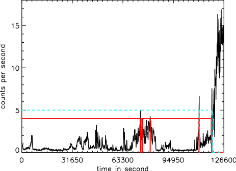
Pulsar J01081431 was observed on 2011 June 15 (MJD 55727) with XMM-Newton (obsid 0670750101) using the European Photon Imaging Camera (EPIC) in Full-Frame mode with the Thin filter. The EPIC-pn (Strüder et al., 2001) and EPIC-MOS1 and MOS2 cameras (Turner et al., 2001) observed the source for 126.7 ks and 127.8 ks respectively. The EPIC data processing was done with the XMM-Newton Science Analysis System (SAS) 11.0222http://xmm.esac.esa.int/sas, applying standard tasks. Our observation was contaminated by soft proton flaring events in the background. We considered different selections of Good Time Intervals (GTIs) for optimal spectral and timing analysis, which are shown in Figure 2 and described in more detail below.
We detected the X-ray counterpart of PSR J01081431 at a position with EPIC-pn.
This position is separated by from the earlier (MJD 54136) Chandra detection at (Pavlov et al., 2009) after accounting for the proper motion by Deller et al. (2009).
The X-ray position differs by from the expected radio pulsar position using the proper motion and VLBI position: (MJD 54100) listed by Deller et al. (2009).
The absolute astrometric error of XMM-Newton is 333XMM calibration document:
http://xmm2.esac.esa.int/docs/documents/CAL-TN-0018.pdf. Thus, the EPIC-pn X-ray position is consistent with the Chandra and VLBI radio position.
2.1. Spectral Analysis
For our spectral analysis of the X-ray counterpart of PSR J01081431, we aimed for the highest possible signal-to-noise ratio, S/N = , where and are the total numbers of counts extracted from the source and background regions of areas and , respectively, and .
Given the strong background flaring in our observation (Figure 2), we tested different GTI filters derived from 100 s binned light-curves of events with energies above 10 and 12 keV for pn and MOS detectors, respectively.
For each GTI-filtered event file, we applied the eregionanalyse task to optimize the aperture size for high S/N spectral extraction. Standard pattern filtering ( 4 for pn and 12 for MOS) was enforced.
We achieved the highest S/N for a GTI count rate cut-off of 5.0 counts s-1 and 0.5 counts s-1 for the pn and MOS light-curves, and for source aperture radii of and for pn and MOS, respectively.
The net GTIs for pn, MOS1 and MOS2 are 104.8 ks, 112.5 ks, and 114.6 ks, respectively.
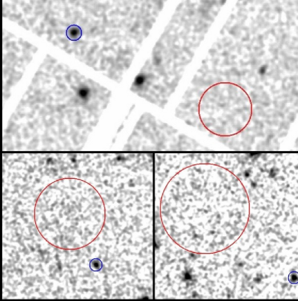
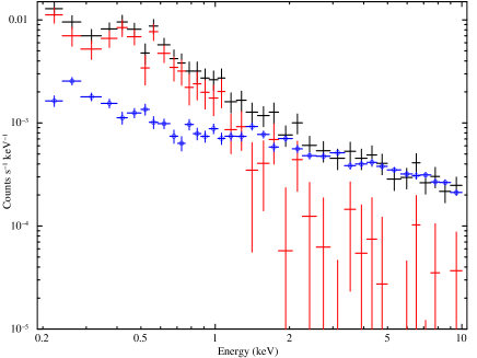
We used larger background regions for better statistics, with the radii of 42′′, 75′′ and 90′′ for pn, MOS1 and MOS2, respectively. The extraction parameters are presented in Table 1. The source and background regions in the three processed EPIC images are shown in Figure 1. The background signal is comparable to the source signal at 1.2 to 2 keV and then exceeds the source signal for energies keV (Figure 3). Considering the substantial count rate errors for the high energies, we restrict our spectral fitting to events in the 0.2–2.5 keV range in order to better constrain the spectral fit parameters.
Considering all three EPIC cameras together, we obtained around 990 total X-ray counts from the source apertures, or around 705 source counts (see Table 1). Redistribution matrices and effective area files were generated using the usual SAS tasks rmfgen and arfgen. For the spectral fit, the SAS task specgroup was used to group the source counts of each spectra with a minimal S/N per bin.
| Extraction parameters | pn | MOS 1 | MOS 2 |
|---|---|---|---|
| Aperture radius | |||
| Energy range (keV) | 0.2 - 2.5 | 0.3 - 2.5 | 0.3 - 2.5 |
| Total aperture counts | 682 | 155 | 152 |
| Source / total counts (%) | 69.9 | 74.0 | 74.4 |
| BG-cor. count rate (ks-1) |
Using XSPEC 12.6.0444http://heasarc.gsfc.nasa.gov/docs/xanadu/xspec, we tested
different spectral models (PL – powerlaw , BB – bbodyrad , BB+PL, BB+BB) applying statistic. For the photoelectric absorption in the interstellar medium (ISM), we used tbabs with the solar abundance table from Anders & Grevesse (1989) and the photoelectric cross-section table from Balucinska-Church & McCammon (1992) together with a new He cross-section based on Yan et al. (1998).
We performed simultaneous fitting of the pn and MOS spectral data.
The values of the fits with separate normalizations for each instrument agreed within the 90% confidence levels with the fit using the same normalization for all instruments.
For simplicity, we give only the latter in the following .
The spectral fit parameters were allowed to vary freely for the single component models, while for the combination of the PL with the BB there were not enough counts for constraining all the parameters sufficiently. Therefore we had to freeze a parameter (see below).
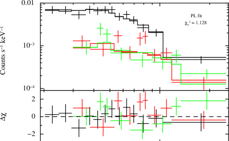
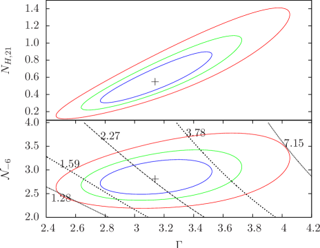
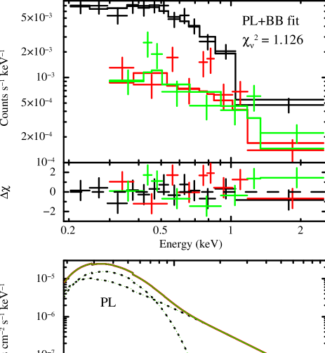
An absorbed PL model with photon index and Hydrogen column density cm-2 provides a good fit of the data with ; see Figure 4 for the X-ray spectral fit and Figure 5 for confidence contours for the three model parameters.
Table 2 lists our best spectral fitting parameters.
The confidence levels for each parameter were obtained using XSPEC’s error and steppar commands.
The non-thermal luminosity is estimated to be erg s-1.
The luminosity uncertainties include both model and distance uncertainties.
| Parameters | Best fit values |
|---|---|
| Absorbed PL fit | |
| ( cm-2) | |
| PL norm ( photons cm-2 s-1 keV-1 at 1keV) | |
| /d.o.f. | 1.1/27 |
| ( erg cm-2 s-1) | |
| ( erg cm-2 s-1) | |
| Absorbed PL+BB fit | |
| ( cm-2) | |
| Fixed | |
| PL norm ( photons cm-2 s-1 keV-1 at 1keV) | |
| (keV) | |
| aafootnotemark: (m) | |
| /d.o.f. | 1.1/26 |
| ( erg cm-2 s-1) | |
| ( erg cm-2 s-1) |
a The radius of the blackbody emission was obtained from the normalization using a distance of pc (Verbiest et al., 2012). Its error is the propagated normalization error only. If one also considers the distance error the correponding values are m.
In contrast to the PL fit, a pure thermal model does not describe the data well.
The best fit of the absorbed BB model has large residuals () that rule out the possibility of the emission being entirely BB-like.
In principle, one could try to fit the spectrum with neutron star atmosphere (NSA) models (Zavlin et al., 1996; Pavlov et al., 1995).
However, the available atmosphere models in XSPEC were calculated either for or strong magnetic fields ( G and higher). For the magnetic field strength of PSR J0108–1431, G, the (redshifted) cyclotron energy is keV. This is too close to the observed photon energy range and has a strong effect on the atmophere spectrum, which is not considered in the weak or strong magnetic field models in XSPEC. Therefore, the NSA models are not applicable for PSR J0108–1431, and we have to stick to the simplistic BB models.
We also checked a two-component BB+BB model with photoelectric absorption. Such a model could describe the thermal emission from a nonuniformly heated neutron star surface. The best fit for this model also has residuals too large to be acceptable ().
A combination of non-thermal magnetospheric emission and thermal emission from polar caps can be modeled by a PL+BB model.
Because of the noise in the data, we had to freeze one fitting parameter.
We froze the photon index to , motivated by the typical photon indices of younger pulsars, (Li et al., 2008). The fit is acceptable (), its BB temperature is keV.
We use the bbodyrad model in XSPEC, whose normalization factor gives the projected area m2 and the corresponding radius of an emitting equivalent sphere, m, where is the distance divided by 210 pc (the errors include only the propagated normalization error), see Table 2 for additional fit results.
Since , the emission likely comes from part of the surface like hot polar caps.
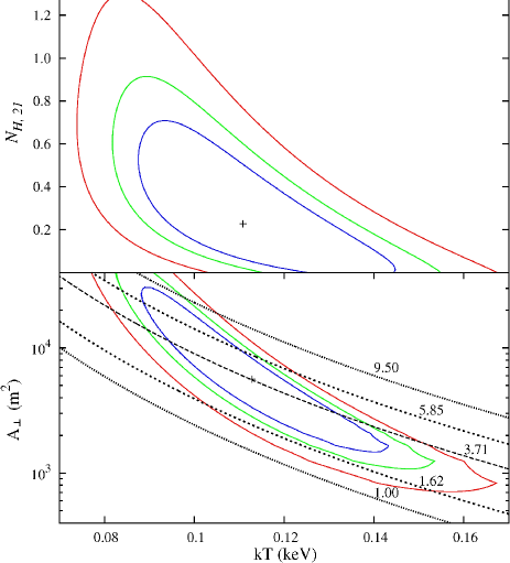
Figure 6 shows the spectral fit and its residuals, while the 68%, 90%, and 99% confidence contours in the – and – planes are plotted in Figure 7. As mentioned above, there are no available atmosphere models for the magnetic field strength of PSR J0108–1431. Therefore, we do no fit a two-component PL+NSA model to the data.
The luminosity for both components together is estimated to be erg s-1. The luminosity of the non-thermal component is erg s-1. The derived values of the temperature and area correspond to the bolometric thermal luminosity of an equivalent sphere erg s-1. The luminosity errors include the propagated distance error and the corresponding propagated fit errors in flux, temperature and emission area. Lines of constant bolometric luminosities are overplotted in the – plane (Figure 7, bottom). The above listed errors of encompass nearly the whole contours in the – plane because we additionally considered the distance error in our conservative error estimate.
2.2. Timing Analysis
Hobbs et al. (2004) reported the radio ephermerides of PSR J01081431 to be Hz and Hz s-1 at MJD . At the start time of our X-ray observations, MJD , the expected frequency change, Hz, is negligible for X-ray timing.
The EPIC-pn detector with a nominal frame time of 73.4 ms in the full frame mode is well suited for the timing analysis of PSR J01081431, while the time resolution of the MOS detectors in full frame mode, 2.6 s, does not allow such an analysis.
Following up on SAS warnings during the data processing, we checked the EPIC-pn CCD with the target on it for time jumps in the data.
We set the SAS environment parameter SAS_JUMP_TOLERANCE555SAS_JUMP_TOLERANCE is given in units of 20.48 s. Only deviations of the measured actual frame time from the nominal frame time larger than the SAS_JUMP_TOLERANCE are identified as time jumps by the SAS. to a value of 33 to account for the known temperature effect on the actual frame time of the EPIC-pn detector (Freyberg et al. 2005, Freyberg et al. 2012666See also: http://www2.le.ac.uk/departments/physics/research/
src/Missions/xmm-newton/technical/leicester-2012-03/freyberg-cal-2012.pdf
).
In addition, we excluded the end of the observation ( ks after start). At that time, a bright X-ray background flare caused the instrument to switch to the counting mode777XMM-Newton Users Handbook, section 3.3.2 – Science modes of the EPIC cameras which resulted in finding of false time jumps by the SAS.
Our final data for the timing analysis were free of apparent time jumps.
All times-of-arrival of the X-ray photons were corrected to the solar barycentric system using the standard task barycen.
We used the test, the sum of powers of first harmonics, (e.g., Buccheri et al. 1983) to search for pulsations in these data. For our timing analysis, we checked 7 different GTI screenings, 11 different energy regions, and 5 different extraction regions in order to maximize the .
The GTI screening with pn count rate counts s-1 for a 100 s binned background light curve (10–12 keV), the extraction radius of 8 ′′, and the energy range of 0.15–2 keV were found to be the optimal choices among the tested variants. At the chosen GTI filter, there is only one small (200 s) time gap in the last fifth of the exposure; see Figure 2.
This filtering provided 507 events during a time span of ks.
PSR J01081431 has been monitored for 16 years, and no glitches have been detected (Espinoza et al., 2011).
Investigating possible timing irregularities for 366 pulsars, Hobbs et al. (2010) found PSR J01081431 to be a very stable pulsar with low timing noise like other pulsars with similarly low . Therefore, we could search for X-ray pulsations at the radio pulsation frequency.
However, to check whether the above-mentioned time jump correction worked properly,
we searched a frequency range of – Hz with a sampling of 0.1 Hz, thus oversampling the expected peak width, Hz, by a factor of 80.
A peak is found at Hz Hz, corresponding to a period of 0.8075647 s s.
The frequency uncertainty was derived similarly to Chang et al. (2012) as .
Within errors the X-ray pulse frequency agrees with the radio pulse frequency very well.
The probability to find by chance is , which corresponds to the confidence level.
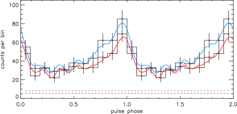
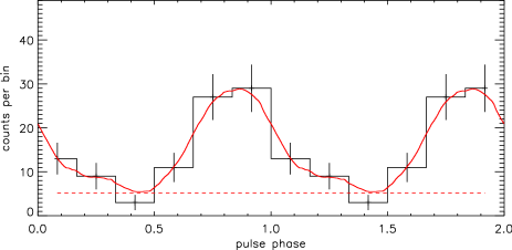
Upper panel: The upper 11-bin histogram represents the full considered energy range, 0.15–2 keV, the corresponding RPA pulse profile is shown in blue, its average background level is indicated with a blue dashed line. Similarly, for the energy range 0.15–1 keV, the red RPA pulse profile corresponds to the lower histogram, and the average background level for this energy range is indicated with a red dashed line. Lower panel: The 6-bin histogram and the RPA pulse profile represent the folded light curve in the energy range 1–2 keV.
To explore the harmonic content of the X-ray pulsations and refine the significance estimate, we performed the test accounting for up to harmonics.
The peak values (and the respective significances) are
(),
(),
(),
(),
(),
() at frequencies consistent within errors with the one found from the test.
For the application of the H-test (de Jager et al., 1989), , we found the to be 48.0, 53.9, 53.5, 54.4, 59.3, 55.5, 56.0 for the first to seventh harmonic, respectively, i.e. the pulsation have statistically significant contributions from 5 leading harmonics of the principal frequency.888We checked up to 20 harmonics as recommended by de Jager et al. (1989) with the same result.
Thus, the pulsations of PSR J01081431 are unambiguously detected in X-rays with a siginificance of .
In order to visualize the pulse shape, we obtained a folded light curve in form of a histogram for the energy range
0.15–2 keV (507 counts), as well as for the splitted energy ranges 0.15–1 keV (416 counts) and 1–2 keV (92 counts).
The frequency Hz, was used for the folding.
We applied the so-called Scott’s rule for setting the upper bound for the histogram bin width by Terrell & Scott (1985). These authors concluded that their rule to avoid oversmoothing gives nearly optimal results for a variety of smooth probability densities. However, choosing the optimal histogram bin size remains a matter of debate in statistical data analysis (for a review, see e.g., Scott 1992). According to Scott’s rule the number of bins must be , where is the number of events. We selected bins for the energy ranges 0.15–2 keV and 0.15–1 keV, and for the energy range 1–2 keV.
The number of counts in the histogram bins depends on the reference phase, which was chosen arbitrarily. The histogram can look quite different for another choice of reference phase, especially if there are few bins.
To obtain the folded light curve independent of the reference phase choice, we averaged the histogram over the reference phase999A similar phase averaging was applied by Zavlin et al. (2002) (their Figure 5)., varying the latter within one histogram bin; see the Appendix A for a short description of the used algorithm.
In the following, we call the obtained new histogram the reference phase averaged (RPA) pulse profile.
The histograms of the folded light curve together with the respective RPA pulse profiles are shown in Figure 8. The pulse shape for the full energy band, 0.15–2 keV, and the soft energy band appear to be asymmetric, with a slower rise and steeper decay. The two RPA pulse profiles have their maxima at similar phases. The 1–2 keV RPA pulse profile appears more sinusodial and slightly shifted to smaller phases compared to the low-energy and broad bands.
However, the pulse shape in the energy range 1–2 keV has poorer statistics, and direct comparisons must be regarded with caution.
Using the RPA pulse profiles as probability distribution templates and the respective number of events as sample sizes, we carried out Monte Carlo simulations of the profiles to estimate the uncertainties of the phase positions of the respective RPA pulse profile maxima.
The maxima of the RPA pulse profiles in Figure 8 are at , , and for the energy ranges 0.15–2 keV, 0.15–1 keV, and 1–2 keV, respectively (see Figure 8).
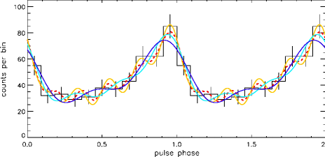
For the full energy band, 0.15–2 keV, for which we have the best statistics, we also use another visualization method. We apply Fourier decomposition up to an harmonic to describe the pulse shape.
| (1) |
where
| (2) |
are one half of the empirical Fourier coefficients, is the phase, is the total number of events in the folded lightcurve, are the event times, and Hz is the pulsation frequency.
The scaling factor allows one to compare the Fourier series plot with the -bin histogram. Here, we apply a scaling factor to
plot the Fourier series for 3, 4 and 5 in Figure 9.
While including five harmonics introduces ‘wiggles’ of the same order as the errors in a light curve bin, Fourier series with coefficients including up to three or four harmonics appear to model well the folded light curve, in particular its asymmetric pulse shape.
From the histograms, we calculate the empirical pulsed fractions as the ratio of the number of counts above the minimum to the total number of counts. For the energy ranges 0.15–2 keV, 0.15–1 keV, and 1-2 keV the pulsed fractions are % %, % %, and % %, and the background-corrected, instrinsic pulsed fractions are % %, % %, and % respectively. We calculated the errors of the pulsed fraction as , following the estimate for broad pulses by de Jager (1994)101010As the power in the fundamental harmonic strongly exceeds the powers in higher harmonics for PSR J01081431, this uncertainty estimate is applicable, albeit approximate..
3. Complementary radio data
It is interesting to compare the radio pulse with the X-ray pulse, in particular the phase difference between them. We use the monitoring radio data described by Weltevrede et al. (2010) for our comparison of the radio and the X-ray profiles. Observations at 1.4 GHz were obtained from December 2009 to July 2012 using the 64-m radio telescope at Parkes, NSW, Australia. The data were calibrated and times-of-arrival (TOAs) produced using psrchive routines (Hotan et al., 2004) and the tempo2 package (Hobbs et al., 2006). An accurate value of the radio dispersion measure (DM) is necessary to correct for the dispersion delay when comparing the relative phases of the 1.4 GHz radio and high-energy pulse profiles. The measured DM for PSR J01081431 is cm-3 pc (Hobbs et al., 2004). This translates into an DM-induced uncertainty of s or in the phase of the radio pulse.
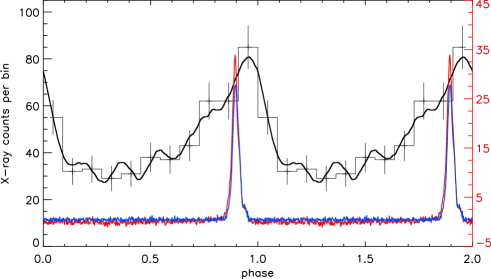
For the comparison with the radio pulse shape, we converted the TOAs of the X-ray photons to the solar system barycenter using the standard SAS task barycen with the same coordinates as in the radio tempo2 analysis and the same DE405 solar-system ephemeris (Standish, 1998). We used the barycentric TOAs of five X -ray events in tempo2 to derive their phases relative to the radio profile. Knowing the X-ray phases of these events as well, we determined the offset between the radio and X-ray phase reference points to be . Correcting for this shift between the reference systems, Figure 10 shows the X-ray and radio profiles together in the same phase range. We confirm the unusual high linear polarization of the radio pulse reported by Weltevrede et al. (2010), obtaining a value of 77% for the fractional linear polarization at the pulse peak. Using the peak positions of the RPA pulse profiles from Section 2.2, the radio pulse leads the X-ray pulse peak by and in the energy ranges 0.15–2 keV and 0.15–1 keV, respectively. In contrast, the X-ray pulse at 1–2 keV leads the radio pulse by . The quoted errors take into account the uncertainties in the reference phase shift, the DM-induced phase uncertainty, the absolute XMM- EPIC-pn timing accuracy of s (Martin-Carrillo et al., 2012), and the dominating error of the maximum position in the RPA pulse profile (Section 2.2).
4. Discussion
4.1. The X-ray spectrum and luminosity
PSR J01081431 is the oldest among the non-recycled ordinary pulsars detected in X-rays, with the spin-down age a factor of 4 larger
than that of PSR B145168, the previous record holder.
It also has the lowest among the same sample of X-ray detected non-recycled pulsars. Our new XMM-Newton observation provided a factor of 20 more source counts enabling better characterization of the pulsar’s spectrum compared to the previous Chandra observation.
However, the strong flaring and high background at energies above keV have undermined energy-resolved timing
and phase-resolved spectral analysis of the pulsar emission.
Formally, a simple absorbed PL model
and an absorbed PL+BB model describe the data equally well.
The photon index (see also Figure 5) of the PL fit is larger (i.e., the spectrum is steeper) than
–2, typical for young pulsars (Li et al., 2008). As mentioned above, for the BB+PL fit we had to freeze one parameter
because of the small number of counts and strong noise.
We chose to fix the photon index at , assuming similar magnetospheric emission characteristics for young and old pulsars.
The PL fit falls in line with the trend observed in other old pulsars, for which the PL fits suggest
too large values in conjunction with
larger photon indices .
For the line of sight of PSR J0108–1431, the LAB Survey of Galactic neutral hydrogen reports cm-2 in this direction (Kalberla et al., 2005), the Dickey & Lockman (1990) neutral hydrogen survey reports cm-2.
The cm-2 from our PL fit is above these total Galactic values.
We use the Lutz-Kelker corrected, parallactic distance pc by Verbiest et al. (2012)
to estimate the expected value applying the ‘analytical’ 3D extinction model described by Posselt et al. (2007). For the close ( pc) solar neighbourhood, this model is based on the 3D Na D absorption line mapping by Lallement et al. (2003) and has a resolution of pc; at larger distances an analytical model is used for the extinction (see Posselt et al. 2007, 2008 for more details).
Considering the errors of the distance, we derived an expected is in the range
(0.3– cm-2.
Assuming 10 H atoms per electron, we derive a similarly low expected cm-2 from the pulsar dispersion measure, pc cm-3 (Hobbs et al., 2004).
Thus,
the absorption is overestimated in the simple PL fit
(see Figure 5) while the 90% confidence range of the parameter in the BB+PL fit includes the expected value.
The temperature obtained in the BB+PL fit, MK, is a reasonable estimate for the expected heated polar cap region.
The effective projected emitting area is m2. This is a factor of smaller than the conventional polar cap area m2, using km.
PSR J01081431 is very similar to other old pulsars in this respect (Posselt et al., 2012; Pavlov et al., 2009; Misanovic et al., 2008; Kargaltsev et al., 2006; Zhang et al., 2005).
We should note, however,
that the values of the temperature and, particularly, the projected area are rather uncertain because of their strong correlation (Figure 7).
As mentioned in the Introduction, one has to take into account that thermal emission from the surface layers of a
neutron star can differ substantially from the BB emission (e.g., Pavlov et al. 1995).
In particular, if the emission emerges from a light-element
(H or He) atmosphere, fitting with neutron star atmosphere models may yield
the effective temperature a factor of 2 lower than ,
and the projected emitting area a factor of 10–100 larger than , while the bolometric luminosity does not change substantially.
The magnetic field can have a strong impact on the observed emission of a neutron star atmosphere. The current neutron star atmosphere models available in XSPEC are not applicable to PSR J0108–1431 because the electron cyclotron line, caused by its magnetic field, G, is in the observable energy range, but it is not included in the XSPEC models. Therefore, we do not discuss atmosphere models for PSR J0108–1431.
Overall, there are now several old pulsars
whose spectra could be described by the PL model,
but the properties of these fits – in particular, the
large and the much higher than expected –
suggest a more complicated model.
Adding a thermal (e.g., BB) component to the spectral model allows lower values and, correspondingly, smaller , similar to those of
younger pulsars.
For comparison with other pulsars, we calculated the non-thermal (PL) luminosity in the 1–10 keV energy range:
erg s-1 for the PL fit,
and erg s-1 for the PL component in the BB+PL fit111111The 1–10 keV
PL component luminosity and its errors were estimated for the fixed ..
The higher photon index of the PL fit, obtained from the fitting at a lower energy range, is the reason why the is smaller in the case of the PL fit than in the case of the PL+BB fit.
The errors were calculated from the 90% confidence errors of the unabsorbed flux and the distance uncertainty of the Lutz-Kelker corrected distance as listed by Verbiest et al. (2012).
These luminosities translate into non-thermal X-ray efficiencies of and for the PL fit and the PL+BB fit, respectively.
Using the bolometric luminosity erg s-1 (Section 2.1), one can also estimate the thermal polar cap heating efficiency from the PL+BB fit,
,
which gives the fraction of spindown power heating the polar caps.
Harding & Muslimov (2001) predicted that the expected polar cap heating efficiency for ordinary pulsars for ages years grows with age and period (e.g., for years, s; see their Figure 7). For pulsars with years they cautioned that the pulsar cannot produce enough electron-positron pairs to fully screen the electric field. Thus, the fraction of the returning positrons that heat the polar cap decreases, and the heating efficiency will drop.
Comparing the estimated polar cap heating efficiency with the predictions by Harding & Muslimov (2001), PSR J01081431 has a lower efficiency than one would expect for a pulsar having the same period (0.8 s) at an age of years.
This could indicate that the returning positron fraction is indeed smaller for PSR J01081431 than for younger pulsars.
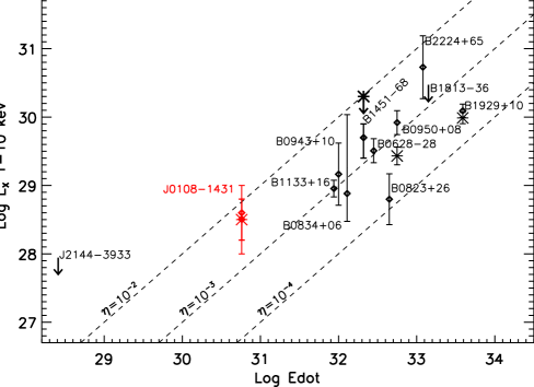
In Figure 11, we updated the X-ray luminosities versus spin-down power plot by Posselt et al. (2012) (their Figure 4121212Note that Posselt et al. (2012) used distances derived from the Lutz-Kelker corrected parallaxes (Verbiest et al., 2010), which differ from the Lutz-Kelker corrected distances. See Verbiest et al. (2012) for details about the differences.). The pulsar again shows properties comparable to those of other old pulsars. In particular, its non-thermal X-ray efficiency is higher than those of young pulsars, most of which have . Thus, the observation that older pulsars seem to radiate in X-rays more efficiently than younger ones (Zharikov et al., 2004; Kargaltsev et al., 2006) is reinforced.
4.2. The X-ray pulsations of PSR J0108–1431
The timing analysis of PSR J0108-1431 (catalog ) establishes, for the first time, unambiguous X-ray pulsations from this pulsar. More than 2 harmonics are required to explain the asymmetric pulse profile.
Such asymmetric pulse profiles can have several explanations, different for
nonthermal and thermal emission.
Asymmetric pulse profiles can be easily produced by nonthermal emission in the outer gap model (Romani & Yadigaroglu, 1995), especially if the special relativity effects, such as aberration and retardation, are taken into account (e.g., Dyks & Rudak 2003 and references therein). A comparison of the detected pulse shapes with those predicted by the models of magnetospheric high-energy emission could be useful in establishing the geometry of the emitting region, especially if additional information about directions of the pulsar’s magnetic and spin axes is available from, e.g., radio-polarimetry. For PSR J01081431, we do not know if the bulk of the observed X-ray emission is produced in the pulsar’s magnetosphere (as it is implied by the PL spectral model), or whether only a high-energy tail originates from the magnetosphere (as we assumed in the PL+BB model). A narrow, sharp pulse would unambiguously point to strongly beamed magnetospheric emission; however, the pulse profile appears to be rather broad (Figure 8) even at higher energies (1–2 keV). Thus, we can neither rule out nor confirm purely non-thermal emission as the cause for the asymmetric pulse profile.
The asymmetric pulse profile can also be produced by thermal emission if
the distributions of temperature and/or magnetic field over the neutron star
surface are not axially symmetric. For instance, an asymmetric pulse with a shape similar to the observed one could be produced by a polar cap whose trailing edge is hotter (hence brighter) than the leading edge, as it was suggested by McGowan et al. (2003) to explain a similar pulse shape for the young ( kyr) PSR J0538+2817.
Another possibility to explain the asymmetric pulse of thermal radiation is
provided by the anisotropy in the local intensity of radiation emerging from
a neutron star atmosphere.
In contrast to the BB radiation, atmospheric
radiation in a strong magnetic field is highly anisotropic, with a ‘pencil component’ along the magnetic field, and ‘fan component’ transverse to the magnetic field (Pavlov et al., 1994).
If the magnetic field is not perpendicular to the
polar cap surface (which can occur if the field is essentially nondipolar), then a great variety of pulse shapes can be produced, depending on the magnetic field inclination and the angle between the spin axis and line of sight.
The strong anisotropy of the atmospheric emission could also explain the relatively
high pulsed fraction of the thermal emission from PSR J01081431. The pulsed fraction % % in the energy range 0.15–1 keV appears to be too high for locally isotropic
BB emission, whose pulsations would be strongly smeared by the bending
of photon trajectories in the gravitational field of the neutron star (Zavlin et al., 1995).
Thus, the properties of the pulsations detected in PSR J0108–1431 do not
contradict to the presence of a thermal component in its emission.
To firmly prove the presence of this component and infer the properties of the polar cap(s) from the comparison with the models, a refined energy-resolved timing
analysis is needed, which would require “cleaner” data.
We found a possible phase shift between the 1.4 GHz and 0.15–2 keV pulse peaks. In principle, it might be due to different emission heights, but the uncertainty of is too large to warrant such an investigation. It is interesting to note, however, that the 1–2 keV RPA pulse profile peak appears to be closer to the radio peak than the 0.15–1 keV RPA pulse profile peak. The 1–2 keV pulse seems to be slightly shifted by from the 0.15–1 keV pulse (considering the maxima of the RPA pulse profiles). In addition, as is apparent from Figure 8, the pulse profile at 1–2 keV appears to be sinusodial while the soft energy pulse profile (0.15–1 keV) is asymmetric. Phase shifts and different pulse shapes would support the hypothesis of two components – an (anisotropic) thermal component and a non-thermal component. However, the high background and the associated large errors prohibit any firm conclusion. It remains to be confirmed, whether or not the two-component model is a viable interpretation, in particular, if a separate non-thermal X-ray component is formed in close vicinity to the radio emission.
5. Summary
We detected for the first time X-ray pulsations of PSR J01081431 at the pulse frequency expected from radio pulse timing. The pulse shape is rather asymmetric, requiring up to 5 harmonics to describe it. The peaks of the radio and the X-ray pulses are close to each other in phase. The X-ray spectrum and the high non-thermal X-ray efficiency of PSR J01081431 are comparable to other old pulsars. In particular, while the spectrum can formally be well described by a PL fit, the expected smaller photon index and lower are better accounted for in a PL+BB model. We were not able to investigate phase-resolved spectra, because of the high background in the strongly flare-impaired observation.
This work was partly supported by NASA grants NNX12AE09G and NNX09AC84G, and by the Ministry of Education and Science of the Russian Federation (contract 11.G34.310001).
Based on observations obtained with XMM-Newton, an ESA science mission with instruments and contributions directly funded by ESA Member States and NASA. The Parkes radio telescope is part of the Australia Telescope which is funded by the Commonwealth Government for operation as a National Facility managed by CSIRO. This research has made use of SAOImage DS9, developed by SAO; the SIMBAD and VizieR databases, operated at CDS, Strasbourg, France; and SAO/NASA’s Astrophysics Data System Bibliographic Services.
Appendix A Obtaining the reference phase averaged pulse profile
In the following, we briefly describe the sliding average bin algorithm used to average over reference phases within one histogram bin, producing the reference phase averaged (RPA) pulse profile. First, we create folded light curve histograms with bins by shifting the reference time in the time series by , where is the period of the pulsations, and is an integer, which is equivalent to shifting the reference phase by . As usual, the bin heights of the histograms are the number of photon counts in the respective bins. Second, we divide the whole phase interval into sub-intervals with bin heights , i.e., there are sub-intervals in each original bin having all the same bin heights. Finally, we average the bin heights of the histograms in each of the sub-intervals:
| (A1) |
For our histograms and RPA pulse profiles in Figure 8, we used , and, as mentioned in Section 2.2, we used bins for the energy ranges 0.15 to 2 keV and 0.15–1 keV, and for the energy range 1-2 keV.
References
- Anders & Grevesse (1989) Anders, E., & Grevesse, N. 1989, Geochim. Cosmochim. Acta, 53, 197
- Balucinska-Church & McCammon (1992) Balucinska-Church, M., & McCammon, D. 1992, ApJ, 400, 699
- Buccheri et al. (1983) Buccheri, R., Bennett, K., Bignami, G. F., et al. 1983, A&A, 128, 245
- Chang et al. (2012) Chang, C., Pavlov, G. G., Kargaltsev, O., & Shibanov, Y. A. 2012, ApJ, 744, 81
- de Jager (1994) de Jager, O. C. 1994, ApJ, 436, 239
- de Jager et al. (1989) de Jager, O. C., Raubenheimer, B. C., & Swanepoel, J. W. H. 1989, A&A, 221, 180
- De Luca et al. (2005) De Luca, A., Caraveo, P. A., Mereghetti, S., Negroni, M., & Bignami, G. F. 2005, ApJ, 623, 1051
- Deller et al. (2009) Deller, A. T., Tingay, S. J., Bailes, M., & Reynolds, J. E. 2009, ApJ, 701, 1243
- Dickey & Lockman (1990) Dickey, J. M., & Lockman, F. J. 1990, ARA&A, 28, 215
- Dyks & Rudak (2003) Dyks, J., & Rudak, B. 2003, ApJ, 598, 1201
- Espinoza et al. (2011) Espinoza, C. M., Lyne, A. G., Stappers, B. W., & Kramer, M. 2011, MNRAS, 414, 1679
- Freyberg et al. (2005) Freyberg, M. J., Burkert, W., Hartner, G. ., Kirsch, M. G. F., & Kendziorra, E. . 2005, in 5 years of Science with XMM-Newton, ed. U. G. Briel, S. Sembay, & A. Read, 159–164
- Harding & Muslimov (2001) Harding, A. K., & Muslimov, A. G. 2001, ApJ, 556, 987
- Harding & Muslimov (2002) —. 2002, ApJ, 568, 862
- Hobbs et al. (2010) Hobbs, G., Lyne, A. G., & Kramer, M. 2010, MNRAS, 402, 1027
- Hobbs et al. (2004) Hobbs, G., Lyne, A. G., Kramer, M., Martin, C. E., & Jordan, C. 2004, MNRAS, 353, 1311
- Hobbs et al. (2006) Hobbs, G. B., Edwards, R. T., & Manchester, R. N. 2006, MNRAS, 369, 655
- Hotan et al. (2004) Hotan, A. W., van Straten, W., & Manchester, R. N. 2004, Publications of the Astronomical Society of Australia, 21, 302
- Kalberla et al. (2005) Kalberla, P. M. W., Burton, W. B., Hartmann, D., et al. 2005, A&A, 440, 775
- Kargaltsev & Pavlov (2008) Kargaltsev, O., & Pavlov, G. G. 2008, in American Institute of Physics Conference Series, Vol. 983, 40 Years of Pulsars: Millisecond Pulsars, Magnetars and More, ed. C. Bassa, Z. Wang, A. Cumming, & V. M. Kaspi, 171–185
- Kargaltsev et al. (2006) Kargaltsev, O., Pavlov, G. G., & Garmire, G. P. 2006, ApJ, 636, 406
- Lallement et al. (2003) Lallement, R., Welsh, B. Y., Vergely, J. L., Crifo, F., & Sfeir, D. 2003, A&A, 411, 447
- Li et al. (2008) Li, X.-H., Lu, F.-J., & Li, Z. 2008, ApJ, 682, 1166
- Manchester et al. (2005) Manchester, R. N., Hobbs, G. B., Teoh, A., & Hobbs, M. 2005, AJ, 129, 1993
- Martin-Carrillo et al. (2012) Martin-Carrillo, A., Kirsch, M. G. F., Caballero, I., et al. 2012, ArXiv e-prints
- McGowan et al. (2003) McGowan, K. E., Kennea, J. A., Zane, S., et al. 2003, ApJ, 591, 380
- Mignani et al. (2008) Mignani, R. P., Pavlov, G. G., & Kargaltsev, O. 2008, A&A, 488, 1027
- Misanovic et al. (2008) Misanovic, Z., Pavlov, G. G., & Garmire, G. P. 2008, ApJ, 685, 1129
- Pavlov et al. (2009) Pavlov, G. G., Kargaltsev, O., Wong, J. A., & Garmire, G. P. 2009, ApJ, 691, 458
- Pavlov et al. (1994) Pavlov, G. G., Shibanov, Y. A., Ventura, J., & Zavlin, V. E. 1994, A&A, 289, 837
- Pavlov et al. (1995) Pavlov, G. G., Shibanov, Y. A., Zavlin, V. E., & Meyer, R. D. 1995, in The Lives of the Neutron Stars, ed. M. A. Alpar, U. Kiziloglu, & J. van Paradijs, 71
- Pavlov et al. (2002) Pavlov, G. G., Zavlin, V. E., & Sanwal, D. 2002, in Neutron Stars, Pulsars, and Supernova Remnants, ed. W. Becker, H. Lesch, & J. Trümper, 273
- Posselt et al. (2012) Posselt, B., Pavlov, G. G., Manchester, R. N., Kargaltsev, O., & Garmire, G. P. 2012, ApJ, 749, 146
- Posselt et al. (2007) Posselt, B., Popov, S. B., Haberl, F., et al. 2007, Ap&SS, 308, 171
- Posselt et al. (2008) —. 2008, A&A, 482, 617
- Romani & Yadigaroglu (1995) Romani, R. W., & Yadigaroglu, I.-A. 1995, ApJ, 438, 314
- Scott (1992) Scott, D. W. 1992, Multivariate Density Estimation
- Standish (1998) Standish, E. M. 1998, A&A, 336, 381
- Strüder et al. (2001) Strüder, L., Briel, U., Dennerl, K., et al. 2001, A&A, 365, L18
- Tauris et al. (1994) Tauris, T. M., Nicastro, L., Johnston, S., et al. 1994, ApJ, 428, L53
- Terrell & Scott (1985) Terrell, G. R., & Scott, D. W. 1985, Journal of the American Statistical Association, 80, pp. 209
- Turner et al. (2001) Turner, M. J. L., Abbey, A., Arnaud, M., et al. 2001, A&A, 365, L27
- Verbiest et al. (2010) Verbiest, J. P. W., Lorimer, D. R., & McLaughlin, M. A. 2010, MNRAS, 405, 564
- Verbiest et al. (2012) Verbiest, J. P. W., Weisberg, J. M., Chael, A. A., Lee, K. J., & Lorimer, D. R. 2012, ArXiv e-prints
- Weltevrede & Johnston (2008) Weltevrede, P., & Johnston, S. 2008, MNRAS, 391, 1210
- Weltevrede et al. (2010) Weltevrede, P., Johnston, S., Manchester, R. N., et al. 2010, Publications of the Astronomical Society of Australia, 27, 64
- Yakovlev & Pethick (2004) Yakovlev, D. G., & Pethick, C. J. 2004, ARA&A, 42, 169
- Yan et al. (1998) Yan, M., Sadeghpour, H. R., & Dalgarno, A. 1998, The Astrophysical Journal, 496, 1044
- Zavlin & Pavlov (2004a) Zavlin, V. E., & Pavlov, G. G. 2004a, ApJ, 616, 452
- Zavlin & Pavlov (2004b) —. 2004b, Mem. Soc. Astron. Italiana, 75, 458
- Zavlin et al. (2002) Zavlin, V. E., Pavlov, G. G., Sanwal, D., et al. 2002, ApJ, 569, 894
- Zavlin et al. (1996) Zavlin, V. E., Pavlov, G. G., & Shibanov, Y. A. 1996, A&A, 315, 141
- Zavlin et al. (1995) Zavlin, V. E., Shibanov, Y. A., & Pavlov, G. G. 1995, Astronomy Letters, 21, 149
- Zhang et al. (2005) Zhang, B., Sanwal, D., & Pavlov, G. G. 2005, ApJ, 624, L109
- Zharikov et al. (2004) Zharikov, S., Shibanov, Y., & Komarova, V. 2004, in 35th COSPAR Scientific Assembly, ed. J.-P. Paillé, Vol. 35, 1914
- Zharikov et al. (2006) Zharikov, S., Shibanov, Y., & Komarova, V. 2006, Advances in Space Research, 37, 1979