Mapping water in protostellar outflows with Herschel

Abstract

Context. Water is a key probe of shocks and outflows from young stars, being extremely sensitive to both the physical conditions associated with the interaction of supersonic outflows with the ambient medium, and the chemical processes at play.

Aims. Our goal is to investigate the spatial and velocity distribution of H₂O along outflows, its relationship with other tracers, and its abundance variations. In particular, this study focuses on the outflow driven by the low mass protostar L1448-C, which previous observations have shown to be one of the brightest H₂O  emitters among the class 0 outflows.

Methods. To this end, maps of the o-H₂O  1₁₀-1₀₁ and 2₁₂-1₀₁ transitions taken with the Herschel-HIFI and PACS instruments, respectively, are presented. For comparison, complementary maps of the CO(3-2) and SiO(8-7) transitions, obtained at the JCMT, and the H₂ S(0) and S(1) transitions, taken from the literature, have been also used. Physical conditions and H₂O  column densities have been inferred with the use of LVG radiative transfer calculations.

Results. The water distribution appears clumpy, with individual peaks corresponding to shock spots along the outflow. The bulk of the 557 GHz line is confined to radial velocities in the range $\pm$10-50  km s^-1, but extended emission at extreme velocities (up to v${}_{r}\sim$ 80  km s^-1) is detected and is associated with the L1448-C extreme high velocity (EHV) jet. The H₂O 1₁₀-1₀₁/CO(3-2) ratio shows strong variations as a function of velocity that likely reflect different and changing physical conditions in the gas responsible for the emissions from the two species. In the EHV jet, a low H₂O/SiO abundance ratio is inferred, that could indicate molecular formation from dust free gas directly ejected from the proto-stellar wind. The ratio between the two observed H₂O  lines, and the comparison with H₂, indicate averaged $T_{kin}$ and $n(H_{2})$ values of $\sim$ 300-500 K and 5 $10^{6}$ cm^-3  respectively, while a water abundance with respect to H₂  of the order of 0.5-1 10^-6 along the outflow is estimated, in agreement with results found by previous studies. The fairly constant conditions found all along the outflow implies that evolutionary effects on the timescales of outflow propagation do not play a major role in the H₂O  chemistry.

Conclusions. The results of our analysis show that the bulk of the observed H₂O  lines comes from post-shocked regions where the gas, after being heated to high temperatures, has been already cooled down to a few hundred K. The relatively low derived abundances, however, call for some mechanism to diminish the H₂O  gas in the post-shock region. Among the possible scenarios, we favor H₂O  photodissociation, which requires the superposition of a low velocity non-dissociative shock with a fast dissociative shock able to produce a FUV field of sufficient strength.

1 Introduction

The earliest stages of star formation are characterized by strong mass loss, which is at the origin of observationally prominent phenomena, such as shocks and molecular outflows. The high velocity of the shocked gas, and the elevated gas temperature, strongly modify the chemical composition of the gas. Depending upon the initial conditions, processes that modify the gas composition include gas dissociation and ionization, high temperature chemical reactions and dust grain reprocessing (e.g. Flower et al. 2010). These processes produce observable signatures in the form of emission from specific molecular and/or atomic lines, the study of which is crucial, not only as a probe of the shock chemistry, but also for understanding the complex interaction between wind/jet-shocks and large scale outflows.

Among the different tracers, lines of H₂  and CO are routinely used to infer the physical conditions and the dynamics of shocked gas, while less abundant molecules, like SiO or CH₃OH, are sensitive to the chemical processes triggered in the shocked gas. In this framework, water can be considered a key molecule: in fact, the H₂O  relative line intensities and its column density are subject to large variations that are highly dependent on both the actual physical conditions of the gas but also on its thermal and chemical history. This is because the water abundance strongly depends on both the mechanism of evaporation/freeze-out in grain mantles and the endothermic gas-phase chemical reactions that drive all free oxygen into water, as well as on the relative timescales of these processes (e.g. Bergin et al. 1998; Flower & Pineau des Forêts 2010).

Observations obtained with the Infrared Space Observatory (ISO) have been the first to detect H₂O  emissions from states of relatively high excitation ($T_{kin}\sim$ 500-1500 K, e.g. Liseau et al. 1996; Ceccarelli et al. 1998; Nisini et al. 2000). More recently, the SWAS and Odin satellites observed the fundamental o-H₂O  transition at 557 GHz in a sample of outflows (Franklin et al. 2008; Bjerkeli et al. 2009; Benedettini et al. 2002). These observations probed cooler gas than had been observed with ISO, but were able to resolve the line profiles for the first time, demonstrating the association of water emission with the high velocity gas. These studies provided the first determinations of the water abundance, yielding values in the range $\sim$ 10^-7 to $\sim$10^-4 and suggesting that the H₂O  abundance depends on both the gas temperature and speed (Giannini et al., 2001; Franklin et al. 2008). However, the strength of this conclusion was limited by the large beam sizes used in these previous observations, together with their limited spectral resolution and/or excitation coverage; these limitations made it difficult to associate enhanced abundances or broadened line profiles with specific regions along the outflows or to infer whether these globally-averaged properties are really representative of the physical and chemical conditions in specific regions of shock activity.

Herschel (Pilbratt et al. 2010) represents the natural evolution for the study of H₂O  in protostellar sources, thanks to the combination of much improved spectral/spatial resolution and sensitivity provided by the PACS (Photodetecting Array Camera and Spectrometer, Poglitsch et al. 2010) and HIFI (Heterodyne Instrument for the Far Infrared, de Graauw et al. 2010) instruments. In the framework of the ”Water In Star-forming regions with Herschel” (WISH, van Dishoeck et al. 2011) key program, we have undertaken systematic PACS and HIFI observations of young outflows in nearby clouds. Within this program, studies of individual shocks have been published in Bjerkeli et al. (2011), Santangelo et al. (2012), Vasta et al. (2012) and Tafalla et al. (2012), while water maps of the L1157 and VLA1623 outflows have been presented in Nisini et al. (2010) and Bjerkeli et al. (2012). All these studies complement observations at the central source position, which probe outflowing gas shocked in the inner jet and envelope cavity walls (Kristensen et al. 2012, Herczeg et al. 2011, Kaska et al. 2012, Goicoechea et al. 2012).

This paper will focus on PACS and HIFI mapping observations of the outflow from the class 0 source L1448-C (also named L1448-mm). This is a low luminosity (L = 7.5 L_⊙; Tobin et al. 2007) protostellar source located in the Perseus Molecular Cloud (D= 232 pc; Hirota et al. 2011), which drives a powerful and highly collimated flow that has been detected through interferometric CO and SiO observations (Guilloteau et al. 1992; Bachiller et al. 1995; Hirano et al. 2010). To the North, the L1448-C outflow interacts with two more compact flows originating from a small cluster of three young sources (L1448-NA, NB and NW, Looney et al. 2000).

Regions of shocked gas are seen along the entire outflow by means of near- and mid-IR of molecular hydrogen emission (Davis & Smith 2006; Neufeld et al. 2009; Giannini et al. 2011), which indicate the presence of a gas at a large range of temperatures, from $\sim$ 300 to more than 2000 K. ISO detected a far-IR spectrum rich in H₂O  and CO transitions towards the L1448-C outflow (Nisini et al. 1999, 2000). The analysis of these lines constrained their emission as coming from warm gas with an enhanced water abundance, as predicted by models for non-dissociative shocks. SWAS and Odin detected the 557 GHz line but at a single-to-noise ratio that was too low to characterize its emission kinematically. These studies, however, suggest that this line might probe a colder water gas component whose abundance is less enhanced with respect to the warm gas. HDO emission at 80.6 GHz has also been detected towards L1448-C, and is associated with both the protostar and the shocked walls of the outflow cavity (Codella et al. 2010b).

Within the WISH program, the L1448-C outflow has been the subject of a detailed study that includes, in addition to the mapping observations presented here, a survey of several lines at specific positions. In particular, Herschel-HIFI observations of the central L1448-C source have been reported by Kristensen et al. (2011), who detected prominent emission originating from both a broad velocity component, probably associated with the interaction of the outflow with the protostellar envelope, and from the Extreme High Velocity gas (EHV, the so-called ”bullets”) associated with the collimated molecular jet. Santangelo et al. (2012) discussed observations carried out towards two specific shock spots, and showed that H₂O  line profiles change significantly with excitation, indicating the presence of gas components having different physical conditions.

The main aims of this work will be to define the global morphological and kinematical properties of the H₂O  emission, in comparison with other standard outflow and shock tracers, and to study abundance variations in the different shocked regions. To this end, complementary CO(3-2) and SiO(8-7) maps of the same region covered by the Herschel observations will be presented and discussed.

2 Observations

2.1 PACS observations

Observations with the PACS instrument were performed on 27 February 2010 (with observing identification number OBSID=1342191349). The PACS Integral Field Unit (IFU) in line spectroscopy mode was used in chopping/nodding mode to obtain a spectral map of the L1448 outflow centered on the H₂O 2₁₂-1₀₁ line at 179.527$\,\mu$m  (i.e. 1669.905 GHz, hereafter referred to as the “179$\,\mu$m  line”). The IFU consists of a 5$\times$5 pixel array providing a spatial sampling of 9$\aas@@fstack{\prime\prime}$4/pixel, for a total field of view of 47$\arcsec\times 47\arcsec$. The diffraction-limited FWHM beam size at 179$\,\mu$m  is 12$\aas@@fstack{\prime\prime}$6. The L1448 outflow region (about $5\arcmin\times 2\arcmin$ centered on the L1448-C(N) source, $\alpha$(J2000) = 03^h25^m38.4^s, $\delta$(J2000) = +30^o44$\arcmin$06$\arcsec$) was covered through a single Nyquist sampled raster map, arranged along the outflow axis. The Herschel pointing accuracy is $\sim$ 2$\arcsec$.

The spectral resolution at 179$\,\mu$m is $R\sim$1500 (i.e. $\sim$210 km s^-1). The observation was performed with a single scan cycle, providing an integration time per spectral resolution element of 30 sec. The total on-source time for the entire map was 5670 sec.

The data were reduced with HIPE v6.0, where they were flat-fielded and flux-calibrated by comparison with observations of Neptune. The calibration uncertainty amounts to around 20-30$\%$, based on cross-calibrations with HIFI and ISO, and on continuum photometry (internal WISH report). Finally, in-house IDL routines were used to locally fit and remove the continuum emission, and to construct an integrated line map.

2.2 HIFI observations

A region of $5\arcmin\times 2\arcmin$ oriented along the direction of the L1448 outflow (PA 164$\degr$) was mapped in the H₂O 1₁₀-1₀₁ line at 556.936 GHz (i.e. 538.29$\,\mu$m, hereafter “the 557 GHz line”) with the HIFI instrument (de Graauw et al. 2010) on 19 August 2010 (OBSID: 1342203200). The On-The-Fly (OTF) mode was adopted, with a distance between adjacent scans of 16$\arcsec$, slightly less than half the diffraction HPBW (which is 38$\arcsec$ at the observed line frequency). The observations were performed in Band 1b with both the Wide Band (resolution 1.1 MHz) and High Resolution (resolution 0.25 MHz) Spectrograph backends (WBS and HRS, respectively), for a total on-source integration time of 3981sec. An inspection of the two sets of data showed that the HRS spectra fail to provide additional information on the line velocity structure, and, furthermore, result in an higher rms noise when smoothed to the resolution of the WBS data (see an example in Fig. 1). Hence in this paper, only the WBS data have been used. The data were reduced using HIPE v7, while further analysis was performed using the GILDAS package. Calibration of the raw data onto the $T_{A}$ scale was performed by the in-orbit system, while the spectra were converted to a $T_{mb}$ scale adopting a main beam efficiency $\eta_{mb}$=0.75 (Roelfsema et al. 2012).

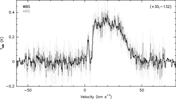
Figure 1: Comparison between a WBS and HRS spectrum at a representative position in the outflow (offsets with respect to L1448-C are indicated). Full black lines show the WBS data, while the gray dotted and full lines show the HRS data before and after smoothing to the WBS resolution, respectively.

Additional analysis consisted of baseline removal in each individual spectrum, averaging of spectra taken during different cycles, and construction of a final data-cube sampled at a regular grid having a half-beam spacing. Observations from the H and V polarizations were separately reduced: spectra from the two polarizations were acquired at slightly different coordinates (offset of $\sim$ 7$\arcsec$) that have been taken into account in constructing the final regridded map. The rms noise achieved in the final data-cube is typically of the order of $T_{mb}\sim$ 0.02 K in a 1  km s^-1  bin.

2.3 JCMT-HARP observations

Complementary CO(3-2) and SiO(8-7) OTF maps were obtained in January 2009 with the HARP-B heterodyne array (Smith et al. 2008) and ACSIS correlator (Dent et al. 2000) on the James Clerk Maxwell Telescope (JCMT). The rest frequencies are 345796.0 and 347330.6 GHz for CO(3-2) and SiO(8-7), respectively (Pickett et al. 1998). The mapped area was covered by consecutive scans in basket-weave mode at a position angle of 160$\degr$. Each scan was offset by 29$\aas@@fstack{\prime\prime}$1 in the orthogonal direction, and the signal was integrated every 7$\aas@@fstack{\prime\prime}$3 (half HPBW, about 14$\arcsec$) along the scan direction. We observed in standard position-switched observing mode, with an off-source position at (+140$\arcsec$, 0$\arcsec$), chosen to be devoid of sources and the presence of high velocity gas. Single maps were co-added and initial data cubes converted into GILDAS format for baseline subtraction and subsequent data analysis. The resulting map is centered on $\alpha_{\rm J2000}$ = 03^h 25^m 38$\aas@@fstack{s}$9 $\delta_{\rm J2000}$ = +30$\degr$ 44$\arcmin$ 05$\aas@@fstack{\prime\prime}$0, and it has dimensions of 300$\arcsec$ $\times$ 116$\arcsec$.

The observed bandwidth, 1 GHz, was sampled with 2048 channels for a spectral resolution of 488 kHz, which corresponds to 0.42 km s^-1 at the observed frequencies. The spectra were smoothed to 1 km s^-1 resolution, to increase the sensitivity, and converted to the main-beam brightness temperature ($T_{\rm mb}$) scale adopting a main-beam efficiency ($\eta_{\rm mb}$) of 0.6. The mean rms noise in $T_{\rm mb}$ is around 100 mK and 80 mK for CO(3-2) and SiO(8-7), respectively.

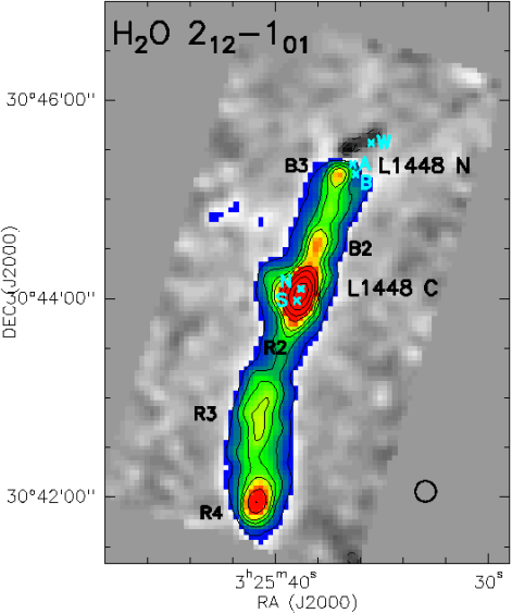
Figure 2: Continuum-subtracted PACS map of the integrated H₂O 2₁₂-1₀₁ emission along the L1448 outflow. Sources in the region are indicated with crosses: L1448-C(S) and C(N) in the central region, and L1448 NA, NB and NW in the northern region. The diffraction-limited beam of FWHM 12.6$\arcsec$ is also indicated. The different emission peaks are labelled following the nomenclature adopted by Bachiller et al. (1990) for individual CO peaks. The average rms noise in the observed region is of the order of 2$\times$10^-6 erg s^-1cm^-2sr^-1 . Contours are drawn at 3$\sigma$, 6$\sigma$,9$\sigma$, 12$\sigma$, 16$\sigma$, 30$\sigma$, 50$\sigma$ and 75$\sigma$. Negative contours are indicated by dashed lines.

3 Results

3.1 H₂O  morphology

The PACS line map displayed in Fig. 2 shows that the 179$\,\mu$m  emission is confined along the L1448-C outflow, with emission peaks roughly located at the positions of shocked spots previously identified through CO and SiO observations; these are named, following the nomenclature of Bachiller et al. (1990), as R1 to R4 and B1 to B3, for the red-shifted and blue-shifted lobes, respectively. The strongest peak is observed towards the central position, where two IR sources, L1448-C(S) and C(N), are located (Jørgensen et al. 2006). Another strong emission peak is also observed in the terminal part of the red-shifted lobe (knot R4). To the north, three different protostellar sources are present, resolved by mm interferometric observations and called A, B and W following Looney et al. (2000) and Kwon et al. (2006). H₂O  emission ends abruptly at the position of L1449 N(A) and N(B), while a lane of water in absorption is seen towards L1448 N(W). Noticeably, and in contrast to what is observed at the central position, no emission is associated with any of the three L1448 N sources. Given the low spectral resolution of the PACS observations, there could be a mixture of emission and absorption beyond the B2 knot causing a near cancellation of the emission.

Figure 3: Upper panel: H₂O 179$\,\mu$m  intensity cut along the L1448 flow, at PA 164$\degr$. The normalized intensity is integrated over a width of 30$\arcsec$ perpendicular to the cut. The location of the C(N) source is taken as the reference for the offsets. Bottom panel: normalized intensities of the 179$\,\mu$m  H₂O  line and continuum, along the same cut direction as above.

Figure 3 shows the line brightness profile along the flow, obtained by integrating the intensity in a region with a width of about 30^′′ perpendicular to the outflow axis. This plot shows the relative intensities of the different emission peaks, indicating that the emission is extended but clumpy.

In the same figure, bottom panel, an enlargement around the L1448-C source is displayed, where the 179$\,\mu$m  line and continuum intensity profiles are compared. In the continuum, the two sources C(S) and C(N) are not spatially resolved: the FWHM of the spatial profile, when fitted with a gaussian, is $\sim$ 18^′′, which means a deconvolved size of $\sim$ 13^′′, assuming both the beam and the emitting region to be gaussian. For comparison, the two sources have a separation of about 8^′′. The line emission appears slightly extended with respect to the continuum, with a deconvolved FWHM of the order of 15^′′. This is roughly similar to the extension of the inner EHV SiO jet as observed, for example, by Guilloteau et al. (1992) and Hirano et al. (2010) (their knots B1/R1). A more detailed description of the water morphology in comparison with other tracers in the regions around the C and N sources is given in Appendix A.

Fig. 4, right panel, presents a comparison of the 179$\,\mu$m  emission, shown as a grayscale image, with the integrated H₂O  557 GHz emission, displayed by separate contours for the blue- and red-shifted emission. The two lines show a similar morphology compatible with the much lower spatial resolution of the HIFI spectra. Indeed, as in the PACS data, bright emission is observed towards the central L1448-C position and the southern, red-shifted outflow lobe, while no water emission is detected north of the L1448-N position. The complete set of HIFI data are presented in Figure B.1, where all the spectra are presented in a regular grid. The comparison between the water and CO peaks can be directly visualized in Fig. 4, left panel, where the 179$\,\mu$m  line map is overlaid with contours of the CO(3-2) emission, separated into the blue- and red-shifted gas. Along the southern outflow, the CO emission is systematically shifted with respect to H₂O. In the northern region, CO extends farthest to the north, where the outflow from the C(N) source is confused with a second outflow (at PA roughly 110$\degr$) emerging from the N(B) source (Bachiller et al. 1990, see next subsection). Therefore, although water roughly follows the direction of the CO outflow, there is not a strict correlation between individual emission peaks.

3.2 H₂O  kinematics

HIFI 557 GHz line profiles at selected positions along the outflows are shown in Fig. 5, and compared with the CO(3-2) line. To make the comparison independent of beam filling effects, the CO(3-2) lines have been extracted from a map convolved to the same spatial resolution of the H₂O 557 GHz observations. All the lines show narrow absorption at the systemic velocity, due to foreground gas. The 557 GHz line always traces the same range of velocity as CO. Maximum velocities up to 50  km s^-1  are detected in all positions, while velocities reaching up to +80 km s^-1  are observed at the position of the L1448-C source; here EHV gas in the form of a separate emission component is clearly detected (Kristensen et al. 2011, see also Fig. 8). Despite tracing the same velocity range, the H₂O  line profiles are different from those of CO, as already shown in other studies (Santangelo et al. 2012; Kristensen et al. 2011): most of the CO emission is localized at low velocity (V${}_{r}-V_{LSR}\la\pm$ 10  km s^-1), while the bulk of the water emission occurs at intermediate velocities (V${}_{r}-V_{LSR}\sim$ 5-30  km s^-1).

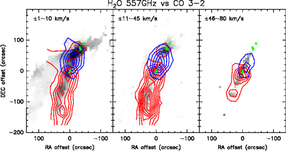
Figure 7: Contours of the H₂O  1₁₀-1₀₁ emission integrated in three different velocity intervals, superimposed onto the CO(3-2) emission in the same velocity bins (gray scale). The velocity ranges with respect to the systemic velocity of V_LSR = 4.7 km s^-1, are shown in the upper side of each panel. Green crosses mark the positions of the different sources (see Fig.1).

A detailed view of the H₂O  and CO emission spatial distribution, as a function of velocity, can be visualized in the velocity channel maps presented in Fig. B.2. Fig. 7 shows the maps of the two emissions integrated in three representative velocity intervals, corresponding to the low ($\pm 1-10$ km s^-1), intermediate ($\pm 11-45$ km s^-1) and high ($\pm 46-86$ km s^-1) velocity gas. Emission at the low and intermediate velocities is detected all along the outflow, with the exception, as already noted from the PACS map, of the region north-west of the L1448-N sources, where water is absent while CO is detected. Fig. 7 also shows that both the H₂O  and CO in the high velocity range ($\ga$ 50 km s^-1) are not confined at the central source position, but extend between $-$100 and +50 arcsec from L1448-C. If we look at the individual spectra shown in Fig. 5, we see that in the CO profiles this EHV gas always appears as a separate ’bullet’ emission superimposed on the line wing at lower velocity (e.g. Bachiller et al. 1990). These EHV bullets are physically associated with the highly collimated molecular jet displaced along the outflow axis (e.g. Hirano et al. 2010). Water emission kinematically associated with these bullets is clearly detected only towards the central L1448-C region (see Fig. 6) and has been discussed in Kristensen et al. (2011). Although EHV emission is also detected at greater distances from the source in CO, this emission does not appear as a separate bullet component in the individual H₂O  spectra, but rather as an extension of the low velocity component wing. Hence the contribution of the EHV gas to the total H₂O  line emission is smaller than in the case of CO. This will be discussed further in the next section.

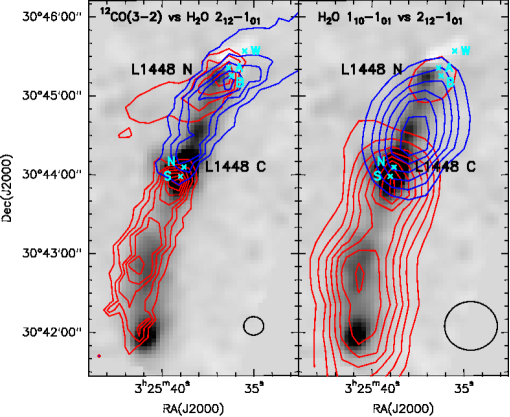
Figure 4: Overlay of the JCMT ¹²CO(3-2) (left panel) and HIFI H₂O  557 GHz (right panel) emission on the H₂O  179$\,\mu$m  map. The blue and red contours represent emission integrated in the velocity ranges ($-$100,$+$4) and ($+$6,$+$100)  km s^-1, respectively. Contours are drawn from 25 to 200 K  km s^-1, with steps of 20 K  km s^-1, for the CO(3-2) map, and from 2 to 12 K  km s^-1, with steps of 1.2 K  km s^-1, for the H₂O 557 GHz map. The HPBW of 14$\arcsec$ (JCMT) and 38$\arcsec$ (HIFI) is indicated.

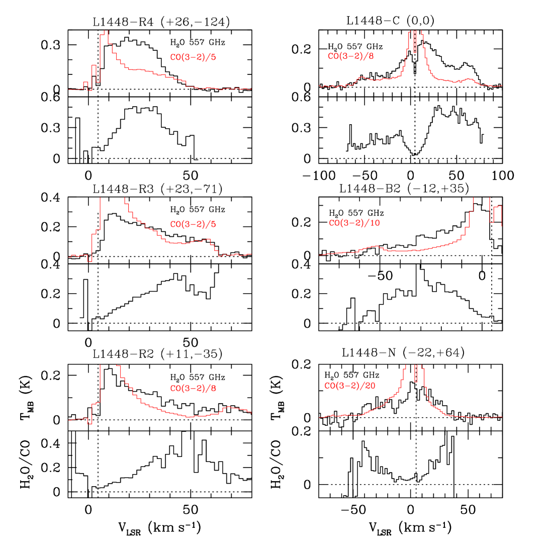
Figure 5: H₂O  1₁₀-1₀₁ (black) and CO(3-2) (red) line profiles at selected outflow positions. CO line profiles, convolved to the H₂O  spatial resolution, have been scaled to match the H₂O  line wings and the corresponding scaling factor is indicated in each plot. At the bottom of each spectrum, the relative H₂O/CO intensity ratio is plotted as a function of velocity.

3.3 H₂O-to-CO ratio vs velocity

As seen in the previous section, the water and CO profiles look different, and thus their ratio varies significantly with velocity as illustrated in Fig 5. At all the selected outflow positions, the H₂O  1₁₀-1₀₁/CO(3-2) ratio increases with velocity up to $v\la$ 20  km s^-1: this is a trend that was identified previously in all sources observed in the 557 GHz line by SWAS and Herschel (Franklin et al. 2008; and Kristensen et al. 2012). Given the high S/N reached in our observations at high velocity, we can now see that beyond 20  km s^-1  the ratio reaches a plateau, and then decreases again at the highest velocities. Variations of the H₂O/CO line ratio could be due both to variations in the physical conditions with velocity and/or to abundance variations. In addition, at velocities close to the ambient velocity, a different degree of absorption of the two lines by the cold gas may influence this ratio. The increase in the H₂O/CO ratio as a function of velocity has been so far interpreted as an increase of the H₂O  abundance at high speeds; assuming the same temperature and density conditions for the two lines, Franklin et al. (2008) derived an H₂O  abundance in the gas with $v_{max}\sim 20$  km s^-1  an order of magnitude higher than that in the low velocity gas. This conclusion, however, was based on an erroneous assumption, since different physical conditions pertain to CO and H₂O; moreover, the physical conditions change with velocity, as shown in, e.g., Santangelo et al. (2012), Vasta et al. (2012) and Lefloch et al. (2010).

Furthermore, the decrease of the H₂O/CO line ratio at velocities larger than $\sim$ 30-40  km s^-1  contradicts the conclusion that a larger water abundance is always associated with the gas at the highest velocity. The drop in the H₂O/CO line ratio roughly coincides with the velocity range of the EHV bullet emission, indicating that a critical change in the physical and/or chemical conditions occurs in the bullets with respect to the ’standard’ wing emission. Tafalla et al. (2010) studied the chemical composition of the EHV gas in L1448, comparing it with the gas responsible for the wing emission, and found significant differences between these two components. They found, in particular, that the EHV gas is relatively rich in O-bearing species and poor in C-bearing molecules compared to the wing regime. Thus the observed drop in the H₂O 1₁₀-1₀₁/CO(3-2) ratio in the EHV regime is more easily understood if the water-emitting EHV gas has a lower temperature and/or density that the gas responsible for the wing emission. Kristensen et al. (2011) compared the excitation conditions for water in the EHV gas with those responsible for the wing emission towards the central position, but were unable to identify significant differences in the two regimes. Santangelo et al. (2012), on the other hand, found that at the L1448-R4 position the high velocity H₂O  emission is associated with gas at a density about an order of magnitude lower than that of the gas responsible for the low velocity emission.

3.4 SiO and H₂O

The SiO(8-7) map, obtained together with the CO(3-2) observations, only shows emission close to the central position, where it can be associated with the L1448-C molecular jet (Hirano et al. 2010). In fact, while SiO emission from the (1-0) and (2-1) transitions is observed along the entire molecular outflow, peaking at the different clump positions (Bachiller et al. 1991, Dutrey et al. 1997), lines at higher excitation are observed only towards the highly collimated micro-jet (Bachiller et al. 1991, Nisini et al. 2007). The comparison of the SiO and H₂O  emissions (see Fig. 6)shows that their profiles are strikingly different. The EHV bullets are more prominent in SiO than in H₂O: conversely, no SiO is associated with the strong intermediate velocity broad H₂O  emission peaking around the ambient velocity. The association of SiO emission with the EHV collimated jet is a well-known feature characteristic of several class 0 sources (e.g. Hirano et al. 2006; Codella et al. 2007); it has been suggested that SiO in the jet is either directly synthesized in the dust-free jet acceleration region (Glassgold et al. 1991; Panoglou et al. 2011) or originates in shocked ambient material where silicon is released into the gas phase by the disruption of grain cores (e.g. Gusdorf et al. 2008).

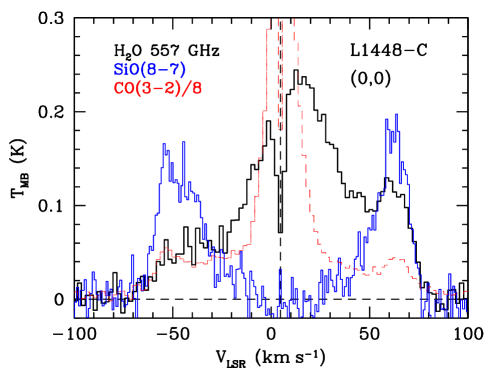
Figure 6: Overlay between H₂O  1₁₀-1₀₁ (black), SiO(8-7) (blue) and CO(3-2) (red) towards the L1448-C position.

An origin in the primary jet has been recently supported by both interferometric observations in the HH212 object (Cabrit et al. 2007) and by the molecular survey conducted on the L1448-R2 EHV bullet by Tafalla et al. (2010), who showed that the bullets possess a peculiar chemistry with respect to the standard outflow wing emission, suggesting an origin different from shocks. The fact that SiO(8-7) is more prominent than H₂O  557 GHz in the EHV bullets may either be an excitation effect or the result of an enhanced SiO/H₂O  abundance ratio, or both. The excitation of SiO in the EHV bullets has been studied by Nisini et al. (2007), who found that the SiO-emitting gas has a density $\sim$ 10⁶ cm^-3  and $T_{kin}\ga$ 300 K. Kristensen et al. (2011) found that similar conditions may be consistent also with the water emission in the bullets, suggesting that SiO and H₂O  are excited in the same gas. With this assumption, the observed H₂O 557 GHz/ SiO(8–7) intensity ratio in the bullets implies a H₂O/SiO abundance ratio of $\sim$ 10. Shock models that take account of the erosion of Si from grain cores and mantles predict this ratio to be of the order of 10³ or more, depending on the shock velocity (Gusdorf et al. 2008; Jiménez-Serra et al. 2008). On the other hand a H₂O/SiO ratio of about 10 is predicted by the wind model of Glassgold et al.(1991) where H₂O  and SiO are formed in dust-free gas directly ejected from the protostar, provided that the mass loss rate of the spherical wind is $>$ 10^-5 M_⊙ yr^-1. Only such high mass loss rates yield a density at the wind base that is high enough to permit efficient SiO synthesis through gas-phase reactions. Indeed, timescales for SiO production are rather low, i.e. they stay below 10² yr, for $T>400K$, only if the gas density is $\ga$10⁷-10⁸cm^-3. Dionatos et al. (2009) measured for the L1448 jet a molecular mass flux rate of $\sim$ 10^-7 M_⊙ yr^-1: for this low mass loss value, the model by Glassgold et al. (1991) predicts a negligible abundance of both SiO and H₂O. However, given the high collimation of the L1448 jet, the mass loss rate values are not directly comparable and certainly the possibility that the two molecules trace the primary jet cannot be ruled out. In this respect, initial results presented in Panoglou et al. (2011) for the molecular survival in disk-winds seem promising, predicting that a significant fraction of water is synthesized in jets from class 0 sources having a mass accretion rate of 5 10^-6 M_⊙ yr^-1, implying a mass flux rate of the order of that measured in L1448.

Finally, we note that the timescales to increase the water abundance to values X(H₂O)$>$10^-5 in a gas with $T>$ 400 K are of the order of 100 yr (Bergin et al. 1998), which match well the dynamical timescale for the L1448 jet propagation of the order of $\sim$ 150 yr (Hirano et al. 2010).

With regards to the broad H₂O  emission at intermediate velocities, Kristensen et al. (2011) suggested an origin in shocks caused by the interaction between the outflow and the envelope. Such shocks would be expected to produce significant SiO emission, since the disruption of grain cores occurs at shock speeds $\ga$ 25-30  km s^-1(Jiménez-Serra et al. 2008; Gusdorf et al. 2008). The efficiency of sputtering and grain-grain collisions, however, depends on the type of grains involved and on the total density: for large grains, sputtering can be significantly inhibited for n(H₂)$\ga$ 10⁶ cm^-3, due to the decrease, at such densities, of the relative velocity between grains and neutral species (Caselli et al. 1997). In fact, the observed SiO(8-7) emission gradually rises from the ambient velocity up to the EHV regime, behaviour which could suggest a progressive enhancement of the SiO abundance moving from the regime of high density and low velocity to that of low density and high velocity; the water, on the other hand, can be efficiently produced even at low shock speeds and high densities from sputtering of icy grain mantles, which would explain the different behavior of the two species in the intermediate velocity regime. However, the non-detection towards L1448-C of broad lines from other molecules residing on ices, such as CH₃OH (Jiménez-Serra et al. 2005), is indicative of the fact that the gas/grain chemistry can indeed be more complex than normally assumed.

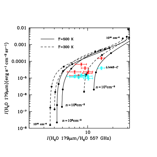
Figure 8: H₂O179$\,\mu$m/557GHz ratio vs the H₂O179$\,\mu$m  intensity (expressed in erg s^-1 cm^-2 sr^-1). Theoretical LVG predictions are plotted for volume densities of 10⁵, 10⁶ and 10⁷ cm^-3, and for kinetic temperatures of 300 K (dashed line) and 500 K (full line). Along each curve the $N$(o-H₂O) column density varies from 10¹² to 10¹⁶ cm^-2  in steps of a factor 10. Filled red squares refer to intensities measured in a beam of 38″, equal to the beam size of the 557 GHz observations. Open cyan circles plot the observed values with the y-axis indicating the unconvolved PACS intensity. The data point for L1448-C is labeled.

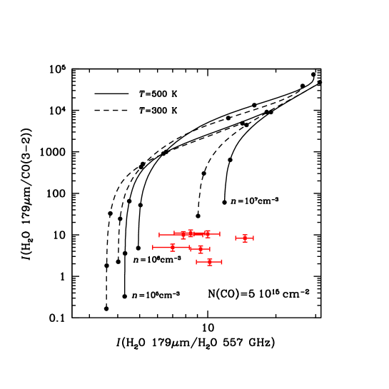
Figure 9: Diagnostic diagram employing the H₂O 179$\,\mu$m/557 GHz vs the H₂O 179$\,\mu$m/CO(3–2) intensity ratios. Theoretical LVG predictions are plotted for the same parameters as in Fig. 8. The plot assumes a fixed $N$(CO) column density of 5 10¹⁵ cm^-2(see text for details). Data points refer to intensities measured in a beam of 38″, equal to the beam of the 557 GHz observations.

4 H₂O physical conditions and abundances

From the relative and absolute intensities of the observed H₂O  lines, it is possible to derive spatially- and spectrally-averaged information about their excitation conditions. For this purpose, we have convolved the PACS line map at the HIFI 557 GHz resolution (i.e. $38\arcsec$), and we have integrated the HIFI spectra over velocity, in order to compare line intensities for the same spatial and spectral regions. In Table 1, we report these intensities, as measured at different positions along the outflow, corresponding roughly to the water intensity peaks.

In Fig. 8, the 179$\,\mu$m  intensity is plotted as a function of the 179$\,\mu$m/557GHz ratio. Here the observed values are confronted with predictions obtained using the RADEX code (van der Tak et al. 2007) that we have run using the Large Velocity Gradient (LVG) approximation in plane-parallel geometry. Based on the analysis presented in Santangelo et al. (2012), Vasta et al. (2012) and Bijerkeli et al. (2012), we assumed that the kinetic temperature ($T_{kin}$) of the gas traced by the observed H₂O  transitions is in the range 300-500 K, similar to that derived by Giannini et al. (2011) from Spitzer observations of the low-lying H₂ transitions. We then explored hydrogen densities ($n_{H_{2}}$) in the range 10⁵-10⁷ cm^-3  and o-H₂O column densities in the range 10¹²-10¹⁶cm^-2. A linewidth of 30 km s^-1  was adopted, representing the typical FWHM of the observed 557 GHz line.

In Fig. 8 H₂O  179$\,\mu$m  intensities, convolved to the 557 GHz resolution, are indicated as filled (red) squares, while open (cyan) squares indicate the unconvolved PACS intensities. The convolved and unconvolved intensities differ by factors between 1.2 and 5, reflecting the extended but clumpy nature of the 179$\,\mu$m  emission as shown in Fig. 3. Assuming that the unconvolved intensities are not further diluted within the PACS beam, Fig. 8, suggests that the density of the gas responsible for the H₂O  emission is in the range $\sim$ 10⁶-10⁷ cm^-3  while the H₂O  column density is $\ga$ 10¹³ cm^-2.

This result is consistent with the work of Santangelo et al. (2012), who analysed Herschel-HIFI spectra of several H₂O  lines gathered towards the L1448-R4 and B2 positions, concluding that the water emission in these positions arises from a gas at T$\sim$ 400-600 K and density of the order of 1-5 10⁶cm^-3. Models with densities lower than 10⁶cm^-3  were not able to fit all the lines observed with HIFI and would require high column densities that are inconsistent with the upper limit on the H${}_{2}^{18}$O observed in the L1448-R4 position. The conditions we derived are also consistent with the results obtained by Tafalla et al. (2012) from an analysis of the o-H₂O  1₁₀-1₀₁ and 2₁₂-1₀₁ emissions in a large sample of shocked spots.

In Fig. 9 the H₂O  data are also compared with the CO(3-2) line intensity, which has been convolved to the HIFI resolution. The expected 179$\,\mu$m/CO(3-2) ratio has been computed for $N({\rm CO})$ = 5 10¹⁵ cm^-2: this value assumes an average $N({\rm H_{2}})$ column density of 5 10¹⁹ cm^-2  along the flow (consistent with the column density estimated in Giannini et al. 2011) and a CO abundance of 10^-4. The figure shows that the observed data are reproduced by a single gas component only for the case of $n({\rm H_{2}})$ $\sim$ 10⁷ cm^-3  and $N({\rm H_{2}O})$ $<$ 10¹² cm^-2. As shown above, such conditions are not consistent with intensities of the 179$\,\mu$m  emission. We also note that the assumed $N({\rm CO})$ is only an upper limit on the beam-diluted CO column density in the assumed 38$\arcsec$ aperture, since the $N({\rm H_{2}})$ has been estimated over a beam of size $\sim$ 10$\arcsec$. To be consistent with the observed ratios, a CO column density one or two order of magnitudes larger than that assumed here would be required, clearly inconsistent with the H₂ observations. This is further and more quantitative evidence that the CO(3-2) and the water emission originate from gas components with different excitation conditions. The low-$J$ CO is likely related to the cold entrained gas and not directly associated with the high temperature shocked gas. Assuming that the CO emission originates in gas at a temperature of the order of 100 K , and with a density of 10⁴cm^-3(e.g. van Kempen et al. 2009), the contribution of the H₂O  557 GHz emission from this gas would be negligible (i.e. 1/10 of the observed beam diluted intensity), even assuming a H₂O/CO abundance $\sim$1. Assuming $T_{kin}\sim$ 500 K and $n_{H_{2}}\sim$ 5 10⁶ cm^-3, o-H₂O  beam-diluted PACS column densities are constrained to be of the order of 10¹³ cm^-2  along the flow, while a higher value, of the order of 10¹⁴ cm^-2  is inferred towards the central position (see Table 1).

To estimate the corresponding H₂O  abundance, we derive $N({\rm H_{2}})$ from the Spitzer spectral image of the H₂ S(1) 17$\,\mu$m  line (Neufeld et al. 2009; Giannini et al. 2011), on the assumption that it originates in the same gas as seen in H₂O by PACS. For this purpose, the H₂ 17$\,\mu$m  image was convolved to the 12″resolution of the PACS map, and the beam-averaged $N({\rm H_{2}})$ was determined assuming the line to be in LTE with T_kin = 500 K. Values of $N({\rm H_{2}})$ of the order of 0.7–6 10¹⁹ cm^-2  are derived for the different positions. Consequently, the water abundance along the outflow is relatively constant with values $\sim$0.5–1$\times$ 10^-6 (see Table 1). For the on-source position, a larger value of $\sim$ 10^-5 is found; however, the large on-source extinction might cause the $N({\rm H_{2}})$ column density to be underestimated, and consequently the X(H₂O) to be overestimated. If we consider as a reference the H₂ S(0) 28$\,\mu$m  emission for deriving the $N({\rm H_{2}})$ towards the central position, we obtain a value of $\sim$ 5 10²⁰ cm^-2  , which would imply X(H₂O)$\sim$ 10^-6. In this case, we should consider this value as a lower limit, since the S(0) emission is likely dominated by gas colder than that giving rise to the water emission observed here.

Table 1: Line intensities^∗ and H₂O abundances

Position	$\int{T_{mb}dv}$ (K  km s-1)			$I$(10-6erg cm-2 s-1 sr-1)			$N$(o-H2O)b	X(H2O)c
(″,″)	H2O	H2O	CO	H2O	H2O	CO	1013cm-2	10-6
	$1_{10}$-$1_{01}$	$2_{21}$-$1_{01}$	$J=$3–2	$1_{10}$-$1_{01}$	$2_{21}$-$1_{01}$	$J=$3–2
($+$26.0,$-$124.1)	10.3	3.2	32.9	1.78	14.9	1.3	3.0	…
($+$29.3,$-$98.2)	7.5	2.8	31.6	1.30	12.9	1.3	1.3	0.7
($+$23.4,$-$71.1)	10.4	2.7	61.3	1.80	12.6	2.5	1.6	0.8
($+$11.1,$-$36.4)	7.9	2.4	26.9	1.37	11.0	1.1	1.0	2
(0,0)	15.7	8.5	115.6	2.72	39.6	4.7	9.0	1-12.0
($-$12.5,$+$34.9)	9.0	3.0	78.05	1.56	14.5	3.2	1.6	0.8
($-$21.7,$+$63.9)	5.4	2.1	104.3	0.93	9.49	4.2	1.8	0.4

We note that the derived abundances are sensitive to the adopted parameters and assumptions. In the regime considered here, the water column densities that we derive depend almost linearly on the assumed H₂  density, which we estimate to be uncertain by a factor of five. Changes in the assumed temperature, on the other hand, will affect both the H₂O  and the H₂  column densities in a similar fashion, having less impact on the derived H₂O  abundance.

5 Origin of the observed emission

Our analysis of the H₂O 1₁₀-1₀₁ and 2₁₂-1₀₁ lines suggests that the gas responsible for the bulk of the H₂O  emission is warm, with T${}_{kin}\sim$ 300- 500 K, and very dense, with $n_{H_{2}}\sim$ 5 10⁶ cm^-3. These parameters, as well as the associated low abundance of $\la$ 10^-6, seem to be typical of the excitation traced by the two H₂O  transitions, since similar physical conditions have been derived for other outflow positions by several authors (e.g. Bjerkeli et al. 2012, Vasta et al. 2012, Tafalla et al. 2012). These physical conditions, along with the observed spatial distribution of the 179$\mu$m emission, indicate that these H₂O  lines mainly trace gas which has been heated and compressed by shocks, rather than entrained ambient gas. This latter possibility was suggested by Franklin et al. (2008) on the basis of SWAS observations, but assuming for the 557 GHz line the same physical parameters as the CO(1-0) line. Our maps have in addition provided evidence that the excitation conditions and abundance of water in L1448 are fairly constant at the sampled spatial scales. This implies very similar shock properties, which seem not to be affected by evolutionary effects on the timescales of outflow propagation. The only exception is the region immediately adjacent to the protostar L1448-C: here an order of magnitude larger H₂O  column density is found relative to the other outflow positions. Part of this on-source emission is associated with the EHV jet where H₂O  and SiO molecules might be directly synthesized in the atomic free protostellar wind (see also Kristensen et al. 2010).

The temperature of few hundred K inferred along the outflow is much lower than the maximum temperature of shocked molecular gas, as traced by H₂  near-IR rovibrational lines ($\sim$ 2000 K), for example. Far-IR H₂O  lines at higher excitation observed by ISO in L1448 indicate the presence of hotter gas with T$\ga$ 1000 K (Nisini et al. 1999, 2000), thus suggesting a distribution of gas temperatures, as has been inferred for the H₂  gas. PACS observations of several young sources suggest that the presence of gas components at different temperatures is indeed very common (e.g. Herczeg et al. 2011; Karska et al. 2012; Goicoechea et al. 2012) and that the H₂O  abundance is typically larger in the hotter gas (Giannini et al. 2001, Santangelo et al. in preparation).

Considering excitation in a single shock, one can expect that different excitation components are associated with different layers in the post-shock region, and that the low-lying H₂O  transitions considered here should trace post-shocked gas layers where the gas has already cooled down to a few hundred K. Santangelo et al. 2012 inferred that the ratios of low excitation H₂O  lines in the L1448-B2 and R4 spots are consistent with non-dissociative J-type shocks, a conclusion also supported by the large inferred densities, which imply a large shock compression factor. In such shocks, as also in C-shocks, high H₂O  abundances are produced in the hot gas, due to the rapid conversion of atomic oxygen into water when $T_{kin}$ exceeds $\sim$ 300-400 K (Kaufman & Neufeld 2006; Flower & Pineau Des Forêts 2010), and should be maintained long after the gas has cooled down. Hence, we should measure the same high H₂O  abundance in both the warm and the hot gas, unless the density is so high to allow a very quick freezeout of gas-phase water onto grain mantles.

For $n_{H_{2}}\sim$ 10⁶ cm^-3, Bergin et al. (1996) derived a timescale $\sim$ 10⁴ yr for this process. Typical timescales for J-shock propagation at a pre-shock density of 10⁴cm^-3  are less than 10² yr and the timescales are not longer than $\sim$ 10³ yr even for C-type shocks; hence grain freeze-out will be of minor importance in reducing the gas-phase water column density in the still warm regions of the post-shocked gas. A water abundance smaller than that expected to result from endothermic gas-phase reactions could result if most of the oxygen not in CO is frozen out in ice mantles in the pre-shock gas. Such a possibility is strongly suggested by the very low abundance of O₂ gas as measured by SWAS and Odin in dense molecular clouds, which indicates that atomic oxygen could be largely depleted (Goldsmith et al. 2000, Larsson et al. 2007). However, ice mantles are quickly destroyed by sputtering for shock speeds exceeding $\sim$ 10-15  km s^-1, so freeze-out within the pre-shock gas can be of relevance only for very slow shocks.

A different way to decrease the H₂O  abundance in the post-shocked gas could be through photodissociation by a pre-existing FUV field. Shock regions located along the outflow cavity wall close to the protostar could be directly exposed to the central source FUV field (e.g. Visser et al. 2012). Far from the source, the only way to produce a significant FUV field is through fast J-type dissociative shocks. This scenario assumes a superposition of two shocks at different velocities: this is expected, e.g., in jet driven outflows where a fast dissociative shock (i.e. the jet shock or Mach disk) decelerates the jet and a low speed shock accelerates the ambient medium (e.g. Raga & Cabrit 1993). The effect of FUV photons, generated by a J-shock, impinging on the region behind a non-dissociative shock has been discussed in Snell et al. (2005). Their result is that these photons are not effective in decreasing the abundance of the hot H₂O  produced at the shock front, since here the timescales for H₂O  formation are extremely short. However, in the post-shocked cooling region, water can be rapidly dissociated and consequently the H₂O  abundance decreases significantly from the peak value at the shock front. Timescales for H₂O  dissociation depend on the strength of the FUV field and the degree of FUV shielding (Lockett et al. 1999). Direct exposure to a radiation field with $G_{0}>\rm few\times 10$ (where $G_{0}$ is the intensity of the radiation field relative to its average interstellar value) returns all the oxygen to atomic form very quickly. If the field is shielded by an $A_{v}\sim 1$ mag, timescales for converting H₂O  back to oxygen are of the order of thousands of years and still compatible with the outflow dynamical timescale. Snell et al. determined that the column of post-shocked H₂O  behind a C-type shock should scale with the FUV field as $\sim 4\times 10^{15}(n_{0}/10^{4}{\rm cm}^{-3})(v_{s}/10\,{\rm km\,s^{-1}})G_{0}^{-1}$, for a shock of velocity $v_{s}$ in gas of pre-shock density 10⁴cm^-3. Our derived column densities of the order of 10¹⁴cm^-2  therefore imply the presence of a FUV field $G_{0}\sim 25(n_{0}/10^{4}\,\rm{cm}^{-3})^{-1}(v_{s}/10\,\rm{km\,s^{-1}})^{-1}\,\rm cm^{-2}$ for such a shock. Further modeling will be required to determine the exact properties of a J-shock capable of producing the necessary FUV field. However, the jet speed (with projected velocity up to 80 km s^-1  along the line of sight) is certainly high enough to drive a J-type shock that emits strongly at FUV wavelengths. The presence of a dissociative shock giving rise to ionizing photons is suggested, in at least specific positions, by the detection of [Fe II] emission along the L1448 outflow by Neufeld et al. (2009) and of OH emission towards the B2 clump (Santangelo et al. 2012). Shocks close to the sources could be instead directly exposed to the source FUV field expanding in the envelope cavity, whose presence is revealed by the scattered light emission detected in the Spitzer IRAC images (Tobin et al. 2007). A different scenario can be also considered, where the hot and warm H₂O  components are actually produced in two separate non-dissociative shocks having different velocities. Slow C-type shocks, with velocities $\la$15 km s^-1  produce post-shocked temperatures that never exceed $\sim$ 300-400 K (e.g. Kaufman & Neufeld 1996): at such temperatures, the conversion of oxygen into water proceeds at very low efficiency and therefore the H₂O  abundance does not dramatically increase relative to its to pre-shock value on the timescale of shock evolution. In addition, as discussed before, at such low velocities ice mantles are not efficiently sputtered; therefore the release of water from grains is also inhibited. Such a scenario would, however, imply that the bulk of the 557 GHz line that we observe originates in a shock having a speed much lower than the actual velocity as measured from the line profile.

6 Conclusions

H₂O  2₁₂-1₀₁ and 1₁₀-1₀₁ maps of the L1448 outflow have been analysed and compared with CO(3–2), SiO(8–7) and H₂  mid-IR lines in order to infer the origin and properties of H₂O  emission in this prototypical class 0 outflow. The main results of our analysis can be summarized as follow:

• On the 12″spatial scale provided by PACS, the 179$\,\mu$m  line distribution appears patchy, with emission peaks localized in shock spots along the outflow. Strong emission is observed towards the L1448-C source, which drives the main outflow in the region, whose spatial extent covers the collimated and compact molecular jet observed in the H₂  S(0) and S(1) lines.

• The kinematical information provided by the 557 GHz HIFI observations reveals that water lines trace the same velocity range as the CO gas, but present a remarkably different profile, which is dominated by emission at intermediate velocities (i.e. $\pm$ 10-30 km s^-1). Emission from gas at extreme velocities (i.e. up to 80 km s^-1) is detected but it is not as prominent as in CO. We analyzed the velocity dependence of the H₂O/CO(3–2) ratio, finding that this ratio varies significantly with velocity. An initial H₂O/CO(3–2) increase is followed by a drop at velocity $\sim$ 30 km s^-1. Such velocity variations are indicative of strong changes in the physical and chemical conditions with the flow speed, and cannot be explained by H₂O  abundance variations alone.

• When compared with SiO(8-7) emission, detected in our map only close to the L1448-C source, H₂O  emission presents significant kinematical differences. SiO is associated only with the EHV gas and it is not detected from the broad H₂O  emission component at intermediate velocity. The low H₂O/SiO ratio inferred in the EHV bullets is not reproduced by shock models and points to an origin from dust-free gas directly ejected from the protostellar wind. The absence of SiO in the broad H₂O  component remains puzzling, however, and could be explained by assuming that grain disruption is inhibited in the very dense H₂O  emitting region.

• From the H₂O  observed line ratio and absolute intensities, and from the additional constraints derived from H₂ lines observed with Spitzer, we infer that the gas responsible for the bulk of the water emission is warm, with $T_{kin}\sim$ 300- 500 K, and very dense, with $n_{H_{2}}\sim$ 5 10⁶ cm^-3. These parameters, as well as the association of the 179$\mu$m emission with specific shock spots, indicates that these H₂O  lines mainly trace gas which has been heated and compressed by shocks and not entrained ambient gas, which instead mainly contributes to the CO(3–2) emission.

• The H₂O  abundance of the gas component traced by the 2₁₂-1₀₁ and 1₁₀-1₀₁ lines has been directly measured comparing the H₂O  column density with the H₂  column density inferred from the H₂  S(1) 17$\,\mu$m  line: values of the order of 0.5–1$\times$10^-6 are found, with small variations along the outflow, but these increase by roughly an order of magnitude towards the L1448-C source. Such a low abundance value, associated with warm gas at a few hundred K, suggests that a diffuse FUV field may act to dissociate the freshly formed water in the post-shock cooling regions. Alternative possibilities, like H₂O  formation in very low-velocity C-type shocks, or freeze-out of H₂O  molecules on dust grains in the post-shocked gas, seem to provide a less compelling explanation of our findings.

Appendix A Comparison of different tracers around the L1448-C and N regions

A.1 L1448-C

Fig. 10 shows an enlargement of the 179$\,\mu$m  emission in the region around L1448-C. Both the continuum and the H₂O  emission are displayed, with superimposed contours of the CO(3-2) and different H₂  lines (Near-IR, from Davis & Smith 1996, and Spitzer from Giannini et al. 2011). The 179$\,\mu$m  line peaks towards the C(N) source but it is elongated along the direction of the molecular jet, as discussed in section 4.1, which in the figure is traced by the H₂ 0–0 S(0) and S(1) lines and comprises the inner peaks in the CO(3-2) emission. The H₂  S(0) line is observed on source and along the SE (red-shifted) jet, while the S(1) line is detected only towards the NW blue-shifted jet and towards the B1 region. Extinction is the likely reason why the S(1) line is not detected on-source. Assuming a temperature of the order of 300 K, the ratio between the S(0) flux and the S(1) upper limit implies a lower limit of A${}_{v}\sim$ 65 mag towards the source and 45 mag in the red-shifted jet.

Finally, Fig. 10 shows the overlay with the H₂  2.12$\,\mu$m  line. At the central source position the line is almost totally extincted and thus no NIR emission is associated with the jet. The 2.12$\,\mu$m  line emission traces instead a bow shock in the blue lobe originated in the interaction of the jet with the ambient medium, which shows up also as a clump of H₂O  emission.

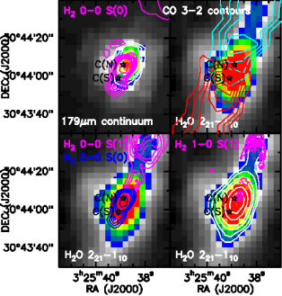
Figure 10: The four panels show maps of the 179$\,\mu$m  line and continuum emission in the region around L1448-C sources, compared with CO(3-2) and H₂  lines at different excitation, namely the 0–0 S(0)(28$\,\mu$m), 0–0 S(1)(17$\,\mu$m), and 1–0 S(1)(2.12$\,\mu$m). White contours, shown in the bottom right and upper left panels, for the line and continuum emission respectively, are drawn at the following values: 1.5, 2.0, 3.0, 4.0, 6.0 8.0 $\times$ 10^-5 erg s^-1cm^-2sr^-1  for the line emission, and 0.6, 0.8, 1.2, 1.6 $\times$ 10^-3 erg s^-1cm^-2sr^-1  for the continuum emission.

A.2 L1448-N

The 179$\,\mu$m  continuum image, displayed in Fig. 11, shows not-resolved emission from the three sources of the L1448-N cluster, having the peak coincident with the N(A) source. Also the H₂  S(0) emission, overlaid on the continuum image, peaks towards N(A), indicating large columns of cold gas. As described in Sect. 3.1, only two of the three sources power outflows, resolved through interferometric observations by Girart et al. (2001) and Kwon et al. (2006). The outflow from N(A) is very compact and it is seen almost perpendicular to the line of sight. By contrast, the outflow from N(B) is more elongated and extends to about 100″  from the driving source (at PA=110$\degr$) both in the blue- and red-shifted lobes. In our CO map we cannot distinguish the blue-shifted gas of these two outflows from the large scale L1448-C main outflow; however, we identify red-shifted emission at velocity between $\sim$ +1 and +20  km s^-1  mainly originating from the N(B) flow (see also Fig. 3, left).

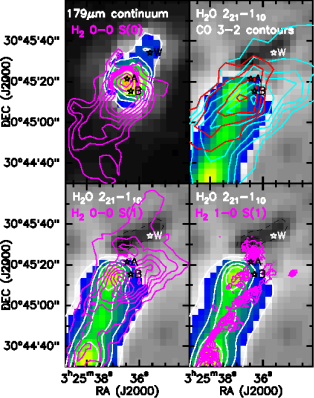
Figure 11: The same as Fig. 10 for a region around L1448-N. In this case, white contours are drawn for the line and continuum emission with the following values: 0.6, 1.2, 1.8, 2.4, 4.0 $\times$ 10^-5 erg s^-1cm^-2sr^-1  (line) and 0.6, 0.8, 1.2, 1.6 $\times$ 10^-3 erg s^-1cm^-2sr^-1  (continuum). A contour of black broken line delineates the absorption region.

In contrast with L1448-C, the 179$\,\mu$m  line emission does not peak towards the sources of this region, but is associated only with the outflow: bright emission is, in particular, observed close to the H₂ S(1) and to the CO(3-2) red-shifted peaks. The bulk of the water emission, however, does not follow the curving H₂  large scale jet driven by L1448-C, but seems to be associated with the 2.12$\,\mu$m  H₂  emission (knots Y/Z in Davis & Smith 1996), excited in the L1448-N(A/B) outflows. This could be a density effect, if one assumes that the density at the base of the N(A/B) flows, is higher than the gas along the large scale jet.

North of the N(A/B) sources the water emission decreases abruptly, while an absorption line of water appears, which follows the 179$\,\mu$m  continuum. The water absorption region lies along the line of sight of the L1448-N reflection nebula, visible in the IR images at both 2.12$\,\mu$m  and in the Spitzer IRAC maps (Davis & Smith 1996, Tobin et al. 2007). This evidence suggests that the cold water in the blue-shifted outflow is seen in absorption against the nebula, which therefore lies in the background.

Appendix B H₂O  557 GHz spectra and velocity channel maps

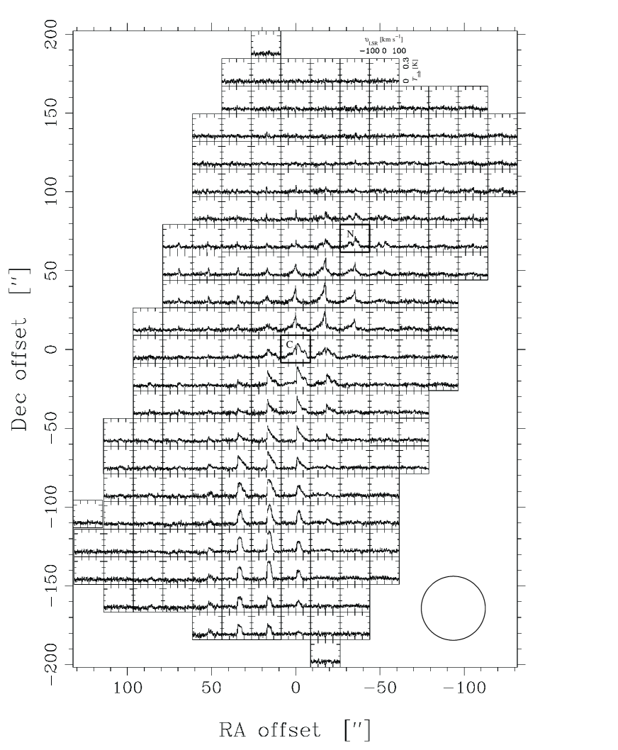
Figure 12: HIFI map of the H₂O  1${}_{10}-1_{01}$ 557 GHz line. The data have been regridded onto a regular grid of 18$\arcsec$ of spacing (i.e. half of the instrumental HPBW, which is displayed in the figure as reference) and binned at 1 km s^-1  resolution. The map is centered on the L1448-C source at $\alpha_{2000}$ = 03^h25^m38.4^s, $\delta_{J}2000$ = +30^o44$\arcmin$06$\arcsec$.

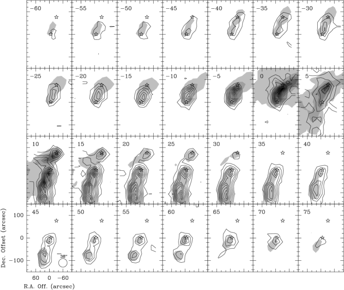
Figure 13: Contours of integrated H₂O557 GHz intensities in velocity intervals of $\Delta V$ = 5  km s^-1  superimposed on gray scale maps of the CO(3-2) intensity integrated in the same bins. The center velocity of the bins is indicated in each panel. H₂O  contours are in steps of 0.03 K  km s^-1  and the first contour is at 0.03 K km s^-1 (equivalent to 3$\sigma$), while CO grey levels are in steps of 1.2 K  km s^-1  and the first contour is at 0.2 K km s^-1. The starred symbols represent the positions of the L1448-C and L1448-N sources.