The new magnetar Swift J1822.3$-$1606

Abstract

On 2011 July 14, a transient X-ray source, Swift J1822.3$-$1606, was detected by Swift BAT via its burst activities. It was subsequently identified as a new magnetar upon the detection of a pulse period of 8.4 s. Using follow-up RXTE, Swift, and Chandra observations, we have determined a spin-down rate of $\dot{P}\sim 3\times 10^{-13}$, implying a dipole magnetic field of $\sim 5\times 10^{13}$ G, second lowest among known magnetars, although our timing solution is contaminated by timing noise. The post-outburst flux evolution is well modelled by surface cooling resulting from heat injection in the outer crust, although we cannot rule out other models. We measure an absorption column density similar to that of the open cluster M17 at 10^′ away, arguing for a comparable distance of $\sim$1.6 kpc. If confirmed, this could be the nearest known magnetar.

1 Introduction

Over the past two decades, several new classes of neutron stars have been discovered. Perhaps the most exotic is that of the magnetars, which exhibit some highly unusual properties, often including violent outbursts and high persistent X-ray luminosities that exceed their spin-down powers.

To date, there are roughly two dozen magnetars and candidates observed, with spin periods between 2 and 12 s, and high spin-down rates that generally suggest dipole $B$-fields of order $10^{13}$ to $10^{15}$ G. Swift has discovered several new magnetars in recent years via their outbursts [Göğüş et al. (2010), Kargaltsev et al. (2012), (e.g. Göğüş et al. 2010; Kargaltsev et al. 2012)].

One of the latest additions to the list of magnetars is Swift J1822.3$-$1606. This source was first detected by Swift Burst Alert Telescope (BAT) on 2011 July 14 (MJD 55756) via its bursting activities [Cummings et al. (2011), (Cummings et al. 2011)]. It was soon identified as a new magnetar upon the detection of a pulse period $P$=8.4377 s [Göğüş et al. (2011), (Göğüş et al. 2011)]. In [Livingstone et al. (2011)], we reported initial timing and spectroscopic results using observations from Swift, Rossi X-ray Timing Explorer (RXTE), and Chandra X-ray Observatory. We found a spin-down rate of $\dot{P}=2.54\times 10^{-13}$ which implies a surface dipole magnetic field $B=4.7\times 10^{13}$ G, the second lowest $B$-field among magnetars. Using an additional 6 months of Swift and XMM-Newton data, [Rea et al. (2012)] present a timing solution and spectral analysis. They find a spin-down rate of $\dot{P}=8.3\times 10^{-14}$ which implies $B=2.7\times 10^{13}$, slightly lower than that found in [Livingstone et al. (2011)]. [Scholz et al. (2012)] present an updated timing solution and latest flux evolution using 46 observations from Swift/XRT, 32 observations from RXTE/PCA, and 5 observations from Chandra/ASIS spanning more than a year. A single archival ROSAT/PSPC observation is also analysed. In these proceedings we summarize the results of [Scholz et al. (2012)].

2 Results

2.1 Timing Behaviour

Table 1: Timing solutions for Swift J1822.3$-$1606.

Parameter	Solution 1	Solution 2	Solution 3
$\nu$ (s-1)	0.1185154253(3)	0.1185154306(5)	0.1185154343(8)
$\dot{\nu}$ (s-2)	$-9.6(3)\times 10^{-16}$	$-2.4(1)\times 10^{-15}$	$-4.3(3)\times 10^{-15}$
$\ddot{\nu}$ (s-3)	-	$1.12(8)\times 10^{-22}$	$4.4(6)\times 10^{-22}$
$\dddot{\nu}$ (s-4)	-	-	$-2.2(4)\times 10^{-29}$
$\chi^{2}_{\nu}/\nu$	5.02/72	1.94/71	1.44/70
$B$ (G)	$2.43(3)\times 10^{13}$	$3.84(8)\times 10^{13}$	$5.1(2)\times 10^{13}$

For each Swift and Chandra observation, a pulse time-of-arrival (TOA) was extracted using a Maximum Likelihood (ML) method, which yields more accurate TOAs than the traditional cross-correlation technique [Livingstone et al. (2009), (see Livingstone et al. 2009)]. For the RXTE observations the cross-correlation method was used, as the high number of counts make the ML method computationally expensive.

Timing solutions were then fit to the TOAs using TEMPO We fit three solutions, one with a single frequency derivative (Solution 1), one with two derivatives (Solution 2) and one with three derivatives (Solution 3). Table 1 shows the best-fit parameters for the three solutions. The addition of higher-order derivatives significantly improves the fit with the solutions having a reduced $\chi^{2}_{\nu}/\nu$ of 5.02/72, 1.94/71, and 1.44/70, respectively. The second and third frequency derivatives serve to fit out the effects of apparent timing noise. The best-fit solution, with three significant derivatives, has a $\nu$ and $\dot{\nu}$ which imply a spin-inferred dipole magnetic field of $5.1(2)\times 10^{13}$ G, the second lowest magnetic field measured for a magnetar thus far. This $B$-field is slightly higher than the value, $2.7\times 10^{13}$ G, measured by [Rea et al. (2012)] as they do not measure significant second and third frequency derivatives. For a detailed comparison of our works see [Scholz et al. (2012)].

2.2 Flux Evolution

We fitted the Swift and Chandra spectra with a blackbody plus power-law model using XSPEC and measured 1–10 keV fluxes. We find a best-fit $N_{H}=4.53(8)\times 10^{21}\,\textrm{cm}^{-2}$ and that the spectrum softens as the flux decays. The flux decay can be characterised by a double-exponential model with decay timescales of $15.5\pm 0.5$ and $177\pm 14$ days.

We find that the observed luminosity decay is also well reproduced by models of thermal relaxation of the neutron-star crust following the outburst. We follow the evolution of the crust temperature profile by integrating the thermal diffusion equation. The calculation and microphysics follow [Brown & Cumming (2009)] who studied transiently accreting neutron stars, but with the effects of strong magnetic fields on the thermal conductivity included [Potekhin et al. (1999), (Potekhin et al. 1999)]. We assume $B=6\times 10^{13}\ {\rm G}$, similar to the value inferred from the spin down and a 1.6 $M_{\odot}$, $R=11.2\ {\rm km}$ neutron star.

We obtain good agreement with the observed light curve for times $<100$ days with an injection of $\sim 3\times 10^{42}\ {\rm ergs}$ of energy at low density $\sim 10^{10}\ {\rm g\ cm^{-3}}$ in the outer crust at the start of the outburst (Figure 2). This conclusion comes from matching the observed timescale of the decay, and is not very sensitive to the choice of neutron-star parameters. We find that it is difficult to match the observed light curve at times $\gtrsim 200$ days, but the late time behaviour is sensitive to a number of physics inputs associated with the inner crust. We will investigate the late-time behaviour in more detail in future work.

2.3 Distance Estimation

Figure 1: A model of the thermal relaxation of the neutron-star crust that approximately reproduces the observed 1–10 keV luminosity decay assuming a distance of 1.6 kpc.

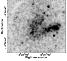
Figure 2: ROSAT image of the field of Swift J1822.3$-$1606 in the 0.1–2.4 keV range. The position of Swift J1822.3$-$1606 is marked by a cross. The large-scale diffuse emission is the Galactic Hii region M17.

As shown in the ROSAT image (Figure 2), the Galactic Hii region M17 is located $\sim$20^′ southwest of Swift J1822.3$-$1606. It has a distance of $1.6\pm 0.3$ kpc [Nielbock et al. (2001), (Neilbock et al. 2001)] and an absorption column density $N_{\rm H}=4\pm 1\times 10^{21}\,$cm ^-2 [Townsley et al. (2003), (Townsley et al. 2003)] which is consistent with our best-fit value of $4.53\times 10^{21}$ cm ^-2. This suggests that Swift J1822.3$-$1606 could have a comparable distance to that of M17. If so, then Swift J1822.3$-$1606 would be one of the closest magnetars detected thus far.

3 Conclusions

We have presented the post-outburst radiative evolution and timing behavior of Swift J1822.3$-$1606. We estimate the surface dipolar component of the $B$-field to be $\sim 5\times 10^{13}$ G, although this measurement is contaminated by timing noise. By applying a crustal cooling model to the flux decay, we found that the energy deposition likely occurred in the outer crust at a density of $\sim 10^{10}$ g cm^-3. Based on the similarity in $N_{H}$ to that of the Hii region M17, we argue for a source distance of $1.6\pm 0.3$ kpc, one of the closest distances yet inferred for a magnetar.

References

- [Brown & Cumming (2009)] Brown, E. F., & Cumming, A. 2009, ApJ, 698, 1020
- [Cummings et al. (2011)] Cummings, J. R., Burrows, D., Campana, S., et al. 2011, The Astronomer’s Telegram, 3488, 1
- [Göğüş et al. (2011)] Göğüş, E., Kouveliotou, C., & Strohmayer, T. 2011, The Astronomer’s Telegram, 3491
- [Göğüş et al. (2010)] Göğüş, E., Cusumano, G., Levan, A. J., et al. 2010, ApJ, 718, 331
- [Kargaltsev et al. (2012)] Kargaltsev, O., Kouveliotou, C., Pavlov, G. G., et al. 2012, ApJ, 748, 26
- [Livingstone et al. (2009)] Livingstone, M. A., Ransom, S. M., Camilo, F., et al. 2009, ApJ, 706, 1163
- [Livingstone et al. (2011)] Livingstone, M. A., Scholz, P., Kaspi, V. M., Ng, C.-Y., & Gavriil, F. P. 2011, ApJ, 743, L38
- [Nielbock et al. (2001)] Nielbock, M., Chini, R., Jütte, M., & Manthey, E. 2001, A&A, 377, 273
- [Potekhin et al. (1999)] Potekhin, A. Y., Baiko, D. A., Haensel, P., & Yakovlev, D. G. 1999, A&A, 346, 345
- [Rea et al. (2012)] Rea, N., Israel, G. L., Esposito, P., et al. 2012, ApJ, 754, 27
- [Scholz et al. (2012)] Scholz, P., Ng, C.-Y., Livingstone, M. A., et al. 2012, ApJ, accepted, arXiv:1204.1034
- [Townsley et al. (2003)] Townsley, L. K., Feigelson, E. D., Montmerle, T., et al. 2003, ApJ, 593, 874