On the Contraction of $so(4)$ to $iso(3)$

Abstract.

For any skew-Hermitian integrable irreducible infinite dimensional representation $\eta$ of $iso(3)$, we find a sequence of (finite dimensional) irreducible representations $\rho_{n}$ of $so(4)$ which contract to $\eta$.

1. Introduction

One of the first known examples of contraction of Lie algebra representations, given in the early work of İnönü and Wigner [1], is the contraction of the representations of the Lie algebra $so(3)$ to those of $iso(2)$. In that example, starting from a sequence, $\left\{\rho_{j}\right\}_{j=1}^{\infty}$ of finite dimensional representations of $so(3)$ with increasing dimension, they obtained an infinite dimensional representation, $\eta_{q}$ of $iso(2)$. They proved the contraction of the representations by the following type of convergence of matrix elements:

$$\lim_{j\longrightarrow\infty}\left\langle{}^{j}_{m^{\prime}}|\rho_{j}(X)|^{j}_{m}\right\rangle=\left\langle{}^{q}_{m^{\prime}}|\eta_{q}(X)|^{q}_{m}\right\rangle$$ (1.1)

where $|^{j}_{m}\rangle$ (respectively $|^{q}_{m}\rangle$) is an element in an orthonormal basis of $\rho_{j}$ (respectively $\eta_{q}$).

In this paper we show that the same type of convergence of matrix elements as in (1.1), holds for the contraction of the finite dimensional irreducible representations of $so(4)$ to infinite dimensional irreducible representations of $iso(3)$. The convergence is proved using a less familiar description of the irreducible representations of $so(4)$ and $iso(3)$, due to Pauli [2].

Our paper is divided as follows: In sections 2 and 3 we will describe the representation theory of $so(4)$ and $iso(3)$ respectively. In section 4 we give the contraction of the algebra $so(4)$ to $iso(3)$ and prove the convergence of the appropriate matrix elements.

2. Representation theory of $so(4)$.

In this section and the one that follows we describe all the skew-Hermitian irreducible finite dimensional representations of $so(4)$ and all the skew-Hermitian irreducible infinite dimensional representations of $iso(3)$. We recall that the Lie algebra $so(4)$ is the direct sum of two copies of the Lie algebra $so(3)$. Moreover every irreducible representation of $so(4)$ is a tensor product of two irreducible representations of $so(3)$. From the work of Weimar-Woods [3, 4] we know all the contractions of representations of $so(3)$ and hence we also know all the contractions of representations of $so(4)$ that respect the decomposition $so(4)=so(3)\oplus so(3)$. As noted in [3], the contraction of $so(4)$ to $iso(3)$ does not respect this decomposition. Hence we use another description of the representations of $so(4)$ which was given by Pauli [2]. The resemblance of the representations of $so(4)$ and $iso(3)$ in this description is more convenient for the contraction procedure. We also give the relation between the parameterization of the irreducible representations as was given by Pauli [2] and the more usual parameterization as a tensor product of two irreducible representations of $so(3)$.

The Lie algebra so(4) can be defined by the basis $\left\{M_{1},M_{2},M_{3},N_{1},N_{2},N_{3}\right\}$ satisfying the following commutation relations:

$$[M_{i},M_{j}]=i\epsilon_{ijk}M_{k}$$ (2.1)

$$[N_{i},N_{j}]=i\epsilon_{ijk}M_{k}$$ (2.2)

$$[M_{i},N_{j}]=i\epsilon_{ijk}N_{k}$$ (2.3)

where $\epsilon_{ijk}$ is the Levi-Civita totally antisymmetric symbol. We will describe all the irreducible finite dimensional integrable representations of $so(4)$ in terms of another basis which is $\left\{M_{+},M_{-},M_{3},N_{+},N_{-},N_{3}\right\}$, where $M_{\pm}=M_{1}\pm iM_{2},N_{\pm}=N_{1}\pm iN_{2}$. $so(4)$ has two independent invariants (Casimir operators) $\vec{M}\cdot\vec{N}$ and $\frac{1}{2}(M^{2}+N^{2})$. On each irreducible representation of $so(4)$, $\vec{M}\cdot\vec{N}$ and $M^{2}+N^{2}$ act as scalar operators with scalars which we denote by $G$ and $F$ respectively. These two scalars determine uniquely (up to an isomorphism) the irreducible representation of $so(4)$. We denote the irreducible representation of $so(4)$ with $F$ and $G$ by $\rho_{F,G}:so(4)\longrightarrow gl(V_{F,G})$. The representation space $V_{F,G}$ has an orthonormal basis of the form $\left\{|^{F,G}_{j,m_{j}}\rangle:j\in\left\{j_{0},j_{0}+1,...,n\right\},m_{j}\in\left\{-j,-j+1,...,j\right\}\right\}$, where $j_{0},n\in\left\{0,\frac{1}{2},1,\frac{3}{2},2,...\right\}$ and they satisfy $G^{2}=j_{0}^{2}(n+1)^{2}$, $2F=j_{0}^{2}+(n+1)^{2}-1$. The dimension of $V_{F,G}$ is given by $\sum_{i=j_{0}}^{n}(2i+1)=(n+1)^{2}-j_{0}^{2}$. The representation $\rho_{F,G}$ is given by:

$$\rho_{F,G}(M_{3})|^{F,G}_{j,m_{j}}\rangle=m_{j}|^{F,G}_{j,m_{j}}\rangle$$ (2.4)

$$\rho_{F,G}(M_{\pm})|^{F,G}_{j,m_{j}}\rangle=\sqrt{(j\mp m_{j})(j\pm m_{j}+1)}|^{F,G}_{j,m_{j}\pm 1}\rangle$$ (2.5)

$$\rho_{F,G}(N_{3})|^{F,G}_{j,m_{j}}\rangle= \alpha^{F,G}_{j}\sqrt{(j+m_{j})(j-m_{j})}|^{F,G}_{j-1,m_{j}}\rangle$$

$$+\beta^{F,G}_{j}m_{j}|^{F,G}_{j,m_{j}}\rangle+$$

$$\alpha^{F,G}_{j+1}\sqrt{(j+m_{j}+1)(j-m_{j}+1)}|^{F,G}_{j+1,m_{j}}\rangle$$

$$\rho_{F,G}(N_{\pm})|^{F,G}_{j,m_{j}}\rangle= \pm\alpha^{F,G}_{j}\sqrt{(j\mp m_{j})(j\mp m_{j}-1)}|^{F,G}_{j-1,m_{j}\pm 1}\rangle$$

$$+\beta^{F,G}_{j}\sqrt{(j\mp m_{j})(j\pm m_{j}+1)}|^{F,G}_{j,m_{j}\pm 1}\rangle$$

$$\mp\alpha^{F,G}_{j+1}\sqrt{(j\pm m_{j}+1)(j\pm m_{j}+2)}|^{F,G}_{j+1,m_{j}\pm 1}\rangle$$

where

$$\beta_{j}^{F,G}=\frac{G}{j(j+1)}$$ (2.8)

$$\alpha_{j}^{F,G}=\sqrt{\frac{2F+1-j^{2}-\frac{G^{2}}{j^{2}})}{(2j+1)(2j-1)}}$$ (2.9)

2.1. $so(4)$ as the direct sum $so(3)\oplus so(3)$

We define $K_{i}\equiv\frac{1}{2}(M_{i}+N_{i}),L_{i}\equiv\frac{1}{2}(M_{i}-N_{i}),i=1,2,3$ and we get a new basis for $so(4)$,
$\left\{K_{1},K_{2},K_{3},L_{1},L_{2},L_{3}\right\}$, satisfying the following commutation relations:

$$\left[K_{i},K_{j}\right]=i\epsilon_{ijk}K_{k}$$ (2.10)

$$\left[L_{i},L_{j}\right]=i\epsilon_{ijk}L_{k}$$ (2.11)

$$\left[K_{i},L_{j}\right]=0.$$ (2.12)

We see that either $\left\{K_{1},K_{2},K_{3}\right\}$ or $\left\{L_{1},L_{2},L_{3}\right\}$ span an ideal of $so(4)$, which is isomorphic to $so(3)$ and hence, $so(4)=so(3)\oplus so(3)$. The invariant operators in terms of this basis are:

$$\vec{M}\cdot\vec{N}=K^{2}-L^{2}$$ (2.13)

$$\frac{1}{2}(M^{2}+N^{2})=K^{2}+L^{2}$$ (2.14)

It is well known that each irreducible finite dimensional representation of $so(4)$ is a tensor product of two irreducible finite dimensional representations of $so(3)$. So for each irreducible representation $\rho_{F,G}:so(4)\longrightarrow gl(V_{F,G})$ there are some $k,l\in\left\{0,\frac{1}{2},1,\frac{3}{2},2,...\right\}$ such that the representation $\rho^{k}\otimes\rho^{l}:so(3)\oplus so(3)\longrightarrow gl(V_{k}\otimes V_{l})$ is isomorphic to $\rho_{F,G}$. The representation $(\rho^{j},V_{j})$ is the unique irreducible representation of $so(3)$ with dimension $2j+1$.
For the irreducible representation of $so(4)$ from Pauli’s description, $\rho_{F,G}$, which is isomorphic to $\rho^{k}\otimes\rho^{l}$, we have the following relations:

$$G=k(k+1)-l(l+1)=\pm j_{0}(n+1)$$ (2.15)

$$F=k(k+1)+l(l+1)=\frac{j_{0}^{2}+(n+1)^{2}-1}{2}$$ (2.16)

$$dimV_{F,G}=dim\left(V_{K}\otimes V_{l}\right)=(2k+1)(2l+1)=$$ (2.17)

$$(n+1)^{2}-j_{0}^{2}=\left(2\sqrt{1+2(F+G)}-1\right)\left(2\sqrt{1+2(F-G)}-1\right)$$

$$n=k+l=-2+\sqrt{1+2(F+G)}+\sqrt{1+2(F-G)}$$ (2.18)

$$j_{0}=|k-l|=|\sqrt{1+2(F+G)}-\sqrt{1+2(F-G)}|$$ (2.19)

$$k=-1+\sqrt{1+2(F+G)}$$ (2.20)

$$l=-1+\sqrt{1+2(F-G)}$$ (2.21)

$$G>0\Longrightarrow l<k,k=\frac{n+j_{0}}{2},l=\frac{n-j_{0}}{2}$$ (2.22)

$$G<0\Longrightarrow l>k,k=\frac{n-j_{0}}{2},l=\frac{n+j_{0}}{2}$$ (2.23)

$$G=0\Longrightarrow l=k=\frac{n}{2},j_{0}=0$$ (2.24)

The two pairs of parameters $(k,l)$ and $(F,G)$ are equivalent and knowing the value of one of these pairs determines uniquely the irreducible representation. The pair $(j_{0},n)$ does not determine uniquely the irreducible representation, but the values of $(j_{0},n)$ along with the knowledge of the sign of $G$ does.

3. Representation theory of $iso(3)$

The Lie algebra $iso(3)$ can be defined by the basis $\left\{J_{1},J_{2},J_{3},P_{1},P_{2},P_{3}\right\}$ satisfying the following commutation relations:

$$[J_{i},J_{j}]=i\epsilon_{ijk}J_{k}$$ (3.1)

$$[P_{i},P_{j}]=0$$ (3.2)

$$[J_{i},P_{j}]=i\epsilon_{ijk}P_{k}$$ (3.3)

We will describe all the skew-hermitian irreducible integrable infinite dimensional representations of $iso(3)$ in the basis $\left\{J_{+},J_{-},J_{3},P_{+},P_{-},P_{3}\right\}$ where $J_{\pm}=J_{1}\pm iJ_{2}$ , $P_{\pm}=P_{1}\pm iP_{2}$. $iso(3)$ has two independent invariants (Casimir operators) $P^{2}$ and $\vec{J}\cdot\vec{P}$. On each irreducible representation of $iso(3)$, $P^{2}$ and $\vec{J}\cdot\vec{P}$ act as scalar operators with the scalars which we denote by $p^{2}$ and $C$ respectively. These two scalars determine uniquely (up to an isomorphism) the irreducible representation of $iso(3)$. We denote the irreducible representation of $iso(3)$ with given $p^{2}$ and $C$ by $\eta_{p^{2},C}:iso(3)\longrightarrow gl(W_{p^{2},C})$. The representation space $W_{p^{2},C}$ has an orthonormal basis of the form $\left\{|^{p^{2},C}_{j,m_{j}}\rangle:j\in\left\{j_{0},j_{0}+1,...\right\},m_{j}\in\left\{-j,-j+1,...,j\right\}\right\}$, where $j_{0}\in\left\{0,\frac{1}{2},1,\frac{3}{2},2,...\right\}$ and they satisfy $C^{2}=j_{0}^{2}p^{2}$. All the $W_{p^{2},C}$ are infinite dimensional. The representation $\eta_{p^{2},C}$ is given by:

$$\eta_{p^{2},C}(J_{3})|^{p^{2},C}_{j,m_{j}}\rangle=m_{j}|^{p^{2},C}_{j,m_{j}}\rangle$$ (3.4)

$$\eta_{p^{2},C}(J_{\pm})|^{p^{2},C}_{j,m_{j}}\rangle=\sqrt{(j\mp m_{j})(j\pm m_{j}+1)}|^{p^{2},C}_{j,m_{j}\pm 1}\rangle$$ (3.5)

$$\eta_{p^{2},C}(P_{3})|^{p^{2},C}_{j,m_{j}}\rangle= \tilde{\alpha}^{p^{2},C}_{j}\sqrt{(j+m_{j})(j-m_{j})}|^{p^{2},C}_{j-1,m_{j}}\rangle$$

$$+\tilde{\beta}^{p^{2},C}_{j}m_{j}|^{p^{2},C}_{j,m_{j}}\rangle+$$

$$\tilde{\alpha}^{p^{2},C}_{j+1}\sqrt{(j+m_{j}+1)(j-m_{j}+1)}|^{p^{2},C}_{j+1,m_{j}}\rangle$$

$$\eta_{p^{2},C}(P_{\pm})|^{p^{2},C}_{j,m_{j}}\rangle= \pm\tilde{\alpha}^{p^{2},C}_{j}\sqrt{(j\mp m_{j})(j\mp m_{j}-1)}|^{p^{2},C}_{j-1,m_{j}\pm 1}\rangle$$

$$+\tilde{\beta}^{p^{2},C}_{j}\sqrt{(j\mp m_{j})(j\pm m_{j}+1)}|^{p^{2},C}_{j,m_{j}\pm 1}\rangle$$

$$\mp\tilde{\alpha}^{p^{2},C}_{j+1}\sqrt{(j\pm m_{j}+1)(j\pm m_{j}+2)}|^{p^{2},C}_{j+1,m_{j}\pm 1}\rangle$$

where

$$\tilde{\beta}_{j}^{p^{2},C}=\frac{C}{j(j+1)}$$ (3.8)

$$\tilde{\alpha}_{j}^{p^{2},C}=\sqrt{\frac{p^{2}-\frac{C^{2}}{j^{2}}}{(2j+1)(2j-1)}}$$ (3.9)

4. Contraction of the matrix elements

In this section, we first recall the definition for contraction and give the contraction of the algebra $so(4)$ to $iso(3)$. Then, for each of the representations $\eta_{p^{2},C}$ we specify a suitable sequence of the representations $\rho_{F(n),G(n)}$ such that we obtain the desired convergence of matrix elements. We will not address the question of contraction of the group representations which was solved by Dooley and Rice [7] and was considered by others [8, 9, 10]. We note that a contraction of the representations of $so(3,1)$ to those of $iso(3)$ was done by Weimar-Woods [11].

4.1. Contraction of $so(4)$ to $iso(3)$

We recall the formal definition for a contraction of Lie algebras. Our notations are similar to those of Weimar-Woods  [12].

Definition 1.

Let $U$ be a complex or real vector space. Let $\mathcal{G}=(U,[\_,\_])$ be a Lie algebra with Lie product $[\_,\_]$. For any $\epsilon\in(0,1]$ let $t_{\epsilon}\in Aut(U)$ ($t_{\epsilon}$ is a linear invertible operator on $U$) and for every $X,Y\in U$ we define

$$[X,Y]_{\epsilon}=t^{-1}_{\epsilon}([t_{\epsilon}(X),t_{\epsilon}(Y)]).$$ (4.1)

If the limit

$$[X,Y]_{0}=\lim_{\epsilon\longrightarrow 0^{+}}[X,Y]_{\epsilon}$$ (4.2)

exists for all $X,Y\in U$, then $[\_,\_]_{0}$ is a Lie product on $U$ and the Lie algebra $\mathcal{G}_{0}=(U,[\_,\_]_{0})$ is called the contraction of $\mathcal{G}$ by $t_{\epsilon}$ and we write $\mathcal{G}\stackrel{{\scriptstyle t(\epsilon)}}{{\rightarrow}}\mathcal{G}_{0}$.

There is an analogous definition  [12] for the case that the limit (4.2) is meaningful only on a sequence:

Definition 2.

Let $U$ be a complex or real vector space, $\mathcal{G}=(U,[\_,\_])$ a Lie algebra with Lie product $[\_,\_]$. For any $n\in\mathbb{N}$ let $t_{n}\in Aut(U)$ and for every $X,Y\in U$ we define

$$[X,Y]_{n}=t^{-1}_{n}([t_{n}(X),t_{n}(Y)]).$$ (4.3)

If the limit

$$[X,Y]_{\infty}=\lim_{n\longrightarrow\infty}[X,Y]_{n}$$ (4.4)

exists for all $X,Y\in U$, then $[\_,\_]_{\infty}$ is a Lie product on $U$ and the Lie algebra $\mathcal{G}_{\infty}=(U,[\_,\_]_{\infty})$ is called the contraction of $\mathcal{G}$ by $t_{n}$ and we write $\mathcal{G}\stackrel{{\scriptstyle t_{n}}}{{\rightarrow}}\mathcal{G}_{\infty}$

Specific examples of contractions of Lie algebras can be found in e.g., [1, 3, 13, 14].

For the $so(4)\rightarrow iso(3)$ case we define the contraction transformation to be $t_{\epsilon}(M_{i})=M_{i}$, $t_{\epsilon}(N_{i})=\epsilon N_{i}$ for every $i\in\left\{1,2,3\right\}$. Then we easily see that:

$$[M_{i},M_{j}]_{0}=i\epsilon_{ijk}M_{k}$$ (4.5)

$$[N_{i},N_{j}]_{0}=0$$ (4.6)

$$[M_{i},N_{j}]_{0}=i\epsilon_{ijk}N_{k}$$ (4.7)

We recall that

$$[J_{i},J_{j}]=i\epsilon_{ijk}J_{k}$$ (4.8)

$$[P_{i},P_{j}]=0$$ (4.9)

$$[J_{i},P_{j}]=i\epsilon_{ijk}P_{k}$$ (4.10)

and we see that the linear map $\psi$, from the contracted Lie algebra, $so(4)_{0}$ to $iso(3)$ which is defined by $\psi(M_{i})=J_{i}$, $\psi(N_{i})=P_{i}$ for $i\in\left\{1,2,3\right\}$ is a Lie algebra isomorphism.

4.2. convergence of the matrix elements

Fix a representation $\eta_{p_{1}^{2},C_{1}}$ of $iso(3)$ and define

$$j_{0}^{1}=\sqrt{\frac{C_{1}^{2}}{p_{1}^{2}}}$$ (4.11)

We define a sequence of representations which consists of some of the representations $\rho_{(F,G)}$, as follows. We take those $\rho_{(F,G)}$ such that the value of their $j_{0}$ parameter equals $j_{0}^{1}$ and such that $sgn(G)=sgn(C_{1})$. There is exactly one irreducible representation for each admissible value of $n$, where the admissible values of $n$ are $I=\left\{j_{0}^{1},j_{0}^{1}+1,j_{0}^{1}+2,...\right\}$. We can describe this sequence by $\left\{(\rho_{(F(n),G(n)},V_{F(n),G(n)})\right\}_{n\in I}$ where

$$G(n)=sgn{(C_{1})}j^{1}_{0}(n+1)$$ (4.12)

$$F(n)=\frac{(j^{1}_{0})^{2}+(n+1)^{2}-1}{2}$$ (4.13)

Before we prove the convergence of matrix elements we need the following technical proposition:

Proposition 1.

For

$${\epsilon}_{n}=\sqrt{\frac{p_{1}^{2}}{2F(n)}}=\sqrt{\frac{p_{1}^{2}}{j_{0,1}^{2}+(n+1)^{2}-1}}$$ (4.14)

the following hold

$$\lim_{n\longrightarrow\infty}\epsilon_{n}\beta^{F(n),G(n)}_{j}=\tilde{\beta}^{p^{2}_{1},C_{1}}_{j}$$ (4.15)

$$\lim_{n\longrightarrow\infty}\epsilon_{n}\alpha^{F(n),G(n)}_{j}=\tilde{\alpha}_{j}^{p^{2}_{1},C_{1}}$$ (4.16)

Proof.

For (4.15) we observe that

$$\lim_{n\longrightarrow\infty}\epsilon_{n}\beta^{F(n),G(n)}_{j}=\lim_{n\longrightarrow\infty}\sqrt{\frac{p_{1}^{2}}{2F(n)}}\frac{G(n)}{j(j+1)}=$$ (4.17)

$$\lim_{n\longrightarrow\infty}\sqrt{\frac{p_{1}^{2}}{(j_{0}^{1})^{2}+(n+1)^{2}-1}}\frac{(sign{(C_{1})}j^{1}_{0}(n+1))}{j(j+1)}=\sqrt{p_{1}^{2}}\frac{(sign{(C_{1})}j^{1}_{0})}{j(j+1)}$$

$$\underbrace{=}_{(\ref{eq4.11})}\sqrt{p_{1}^{2}}\frac{(sign{(C_{1})}\sqrt{\frac{C_{1}^{2}}{p_{1}^{2}}})}{j(j+1)}=\frac{C_{1}}{j(j+1)}=\tilde{\beta}_{j}^{p^{2}_{1},C_{1}}$$

(4.16) is obtained similarly. ∎

Theorem 1.

For any $|^{F(n),G(n)}_{j,m_{j}}\rangle$, $|^{F(n),G(n)}_{\tilde{j},\tilde{m}_{\tilde{j}}}\rangle$ $\in V_{F(n),G(n)}$ and any
$X\in so(4)$

$$\lim_{n\rightarrow\infty}\left\langle{}^{F(n),G(n)}_{\tilde{j},\tilde{m}_{\tilde{j}}}|\rho_{F(n),G(n)}(t_{n}(X))|^{F(n),G(n)}_{j,m_{j}}\right\rangle=$$ (4.18)

$$\left\langle{}^{p^{2}_{1},C_{1}}_{\tilde{j},\tilde{m}_{\tilde{j}}}|\eta_{p^{2}_{1},C_{1}}(\psi(X))|^{p^{2}_{1},C_{1}}_{j,m_{j}}\right\rangle$$

where $t_{n}=t(\epsilon_{n})$.

Proof.

We note that from linearity it is enough to prove that (4.18) holds for $X\in\left\{M_{+},M_{-},M_{3},N_{+},N_{-},N_{3}\right\}$. We have:

$$\lim_{n\longrightarrow\infty}\left\langle{}^{F(n),G(n)}_{j,m_{j}}|\rho_{F(n),G(n)}(t_{n}(M_{3}))|^{F(n),G(n)}_{j,m_{j}}\right\rangle=$$ (4.19)

$$\lim_{n\longrightarrow\infty}\left\langle{}^{F(n),G(n)}_{j,m_{j}}|m_{j}|^{F(n),G(n)}_{j,m_{j}}\right\rangle=m_{j}=\left\langle{}^{p^{2}_{1},C_{1}}_{j,m_{j}}|\eta_{p^{2}_{1},C_{1}}(\psi(M_{3}))|^{p^{2}_{1},C_{1}}_{j,m_{j}}\right\rangle$$

$$\lim_{n\longrightarrow\infty}\left\langle{}^{F(j),G(j)}_{j,m_{j}\pm 1}|\rho_{F(n),G(n)}(t_{n}(M_{\pm}))|^{F(n),G(n)}_{j,m_{j}}\right\rangle=$$ (4.20)

$$\lim_{n\longrightarrow\infty}\sqrt{(j\mp m_{j})(j\pm m_{j}+1)}=\sqrt{(j\mp m_{j})(j\pm m_{j}+1)}=$$

$$=\left\langle{}^{p^{2}_{1},C_{1}}_{j,m_{j}\pm 1}|\eta_{p^{2}_{1},C_{1}}(\psi(M_{\pm}))|^{p^{2}_{1},C_{1}}_{j,m_{j}}\right\rangle$$

$$\lim_{n\longrightarrow\infty}\sum_{k=-1}^{1}{\langle^{F(n),G(n)}_{j+k,m_{j}}|\rho_{F(n),G(n)}(t_{\epsilon_{n}}(N_{3}))|^{F(n),G(n)}_{j,m_{j}}\rangle}=$$ (4.21)

$$\lim_{n\longrightarrow\infty}\epsilon_{n}\alpha_{j}^{F(n),G(n)}\sqrt{(j+m_{j})(j-m_{j})}+\epsilon_{n}\beta^{F(n),G(n)}_{j}m_{j}|^{F(n),G(n)}_{j,m_{j}}+$$

$$\epsilon_{n}\alpha^{F(n),G(n)}_{j+1}\sqrt{(j+m_{j}+1)(j-m_{j}+1)}=$$

$$\tilde{\alpha}_{j}^{p_{1}^{2},C_{1}}\sqrt{(j+m_{j})(j-m_{j})}+\tilde{\beta}^{p_{1}^{2},C_{1}}_{j}m_{j}|^{F(n),G(n)}_{j,m_{j}}+$$

$$\tilde{\alpha}^{p_{1}^{2},C_{1}}_{j+1}\sqrt{(j+m_{j}+1)(j-m_{j}+1)}=\sum_{k=-1}^{1}{\langle^{p^{2}_{1},C_{1}}_{j+k,m_{j}}}|\eta_{p^{2}_{1},C_{1}}(\psi(N_{3}))|^{p^{2}_{1},C_{1}}_{j,m_{j}}\rangle$$

where we have used proposition 1. Similarly:

$$\lim_{n\longrightarrow\infty}\sum_{k=-1}^{1}{\langle^{F(n),G(n)}_{j+k,m_{j}\pm 1}}|\rho_{F(n),G(n)}(t_{\epsilon_{n}}(N_{\pm}))|^{F(n),G(n)}_{j,m_{j}}\rangle=$$ (4.22)

$$\lim_{n\longrightarrow\infty}\pm\epsilon_{n}\alpha^{F(n),G(n)}_{j}\sqrt{(j\mp m_{j})(j\mp m_{j}-1)}+$$

$$\epsilon_{n}\beta^{F(n),G(n)}_{j}\sqrt{(j\mp m_{j})(j\pm m_{j}+1)}\mp$$

$$\epsilon_{n}\alpha^{F(n),G(n)}_{j+1}\sqrt{(j\pm m_{j}+1)(j\pm m_{j}+2)}=\pm\tilde{\alpha}^{p_{1}^{2},C_{1}}_{j}\sqrt{(j\mp m_{j})(j\mp m_{j}-1)}+$$

$$\tilde{\beta}^{p_{1}^{2},C_{1}}_{j}\sqrt{(j\mp m_{j})(j\pm m_{j}+1)}\mp\tilde{\alpha}^{p_{1}^{2},C_{1}}_{j+1}\sqrt{(j\pm m_{j}+1)(j\pm m_{j}+2)}=$$

$$\sum_{k=-1}^{1}\langle^{p^{2}_{1},C_{1}}_{j+k,m_{j}\pm 1}|\eta_{p^{2}_{1},C_{1}}(\psi(N_{\pm}))|^{p^{2}_{1},C_{1}}_{j,m_{j}}\rangle$$

All the other matrix elements vanish and obviously satisfy (4.18). ∎

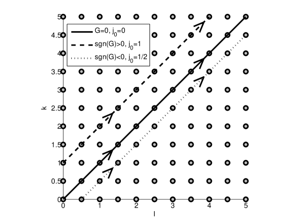
Figure 1. Grid of $so(4)$ finite dimensional irreducible representations and some of their contractions. Note the sign conventions indicated in the box (upper left insert).

4.3. Graphical representation of the contraction process

In figure 1 each point with coordinates $(k,l)$ represents the irreducible representation of $so(4)$ which we denoted by $\rho^{k}\otimes\rho^{l}$. In each ”diagonal” line, $j_{0}$ is constant and equal to the value of $|k-l|$ (those are the lines $k-l=\pm j_{0}$ in the $k,l$ plane). Going along each diagonal line in the direction of the arrow (which is equivalent to taking $\epsilon_{n}$ to zero) we are increasing the value of $n$ by one unit at each step , and this is the picture of the contraction. The solid, dashed and dotted diagonal lines correspond to contractions toward $\eta_{p^{2},C}$ with their $j_{0}$ parameter equal to $0,1$ and $\frac{1}{2}$ respectively.

5. Discussion

The four-dimensional rotation group, $SO(4)$ occurs as a symmetry group of a physical system. The best known example is as the symmetry group of the Hydrogen atom. The group of isometries of the three-dimensional space, $\mathbb{R}^{3}$ i.e., the Euclidean group $ISO(3)$ is another group that is naturally related to many physical systems. Among others, $ISO(3)$ is a subgroup of both Poincaŕe group and Galilei group. The relation between $SO(4)$ and $ISO(3)$ was only partially studied, e.g., [15, 16, 17].
In another work [18, 19] we give a definition for contraction of Lie algebra representations using the notion of direct limit. We also show there that the convergence of matrix elements implies the convergence in norm of the sequence of operators. This shows that the contraction we obtained here is also a contraction according to the definition in [18].

Acknowledgments
AM is grateful to Prof. Weimar-Woods for a helpful discussion.
EMS would like to thank Mr. ShengQuan Zhou for sharing his notes on the contractions of $so(4)$.
The research of the 2nd author was supported by the center of excellence of the Israel Science Foundation grant no. 1438/06.
JLB thanks the Department of Physics, Technion, for its warm hospitality and support during visits while this work was being carried out, and the FRAP-PSC-CUNY for some support.

References

• [1] E. Δ°nΓΆnΓΌ and E. P. Wigner, On the contraction of groups and their representations Proc. Nat. Acad. Sci. U.S 39 (1953), 510-24.
• [2] W. Pauli, Continuous groups in quantum mechanics Ergeb. Exakt. Naturwiss. 37 (1965), 85-104.
• [3] E. Weimar-Woods, The three-dimensional real Lie algebras and their contractions J. Math. Phys. 32 (1991), 2028-33.
• [4] E. Weimar-Woods, Contraction of Lie algebra representations J. Math. Phys. 32 (10) (1991), 2660-5.
• [5] S. F. Singer, Linearity, Symmetry and Prediction in the Hydrogen Atom Springer (2005), p 259.
• [6] D. M. Brink and G. R. Satchler, Angular Momentum Oxford Science Publications, third edition (1993), p 15.
• [7] A. H. Dooley and J. W. Rice, Contractions of rotation groups and their representations Math. Proc. Camb. Phil. Soc. 94 (1983), 509-17.
• [8] K. B. Wolf, Recursive method for the computation of the $SO(n)$, $SO(n,1)$, and $ISO(n)$ representation matrix elements J. Math. Phys. 12 (1971), 197-206.
• [9] M. K.F. Wong and H. Y. Yeh, Explicit evaluation of the representation functions of $ISO(n)$ J. Math. Phys. 21 (1980), 1-5.
• [10] M. K.F. Wong and H. Y. Yeh, A unified treatment of the representation functions of $SO(n,1)$, $SO(n+1)$ and $ISO(n)$ J. Math. Phys. 22 (1981), 1559-1565.
• [11] E. Weimar-Woods, The general structure of G-graded contraction of Lie algebras II: the contracted Lie algebra Rev. Math. Phys. 18 (6) (2006), 655-711.
• [12] E. Weimar-Woods, Contractions, generalized Δ°nΓΆnΓΌ-Wigner contractions and deformations of finite-dimensional Lie algebras Rev. Math. Phys. 12 (11) (2000), 1505-29.
• [13] E. J. Saletan, Contraction of Lie groups J. Math. Phys. 2 (1) (1961), 1-21.
• [14] Robert Gilmore, Lie Groups, Lie Algebras and Some of Their Applications, Dover Publications, Inc. (2005), 436-477.
• [15] W. J. Holman, The asymptotic forms of the Fano function: The representation functions and Wigner coefficients of SO(4) and E(3) Ann. Phys. 52 (1969).
• [16] M. Levy-Nahas and R. Seneor, First order deformations of Lie algebra representations, E(3) and PoincarΓ© examples Commun. Math. Phys. 9 (1968), 242-266.
• [17] A. I. Bobenko, Euler equations in the algebras $e(3)$ and s​o​(4)π‘ π‘œ4so(4). Isomorphisms of integrable cases Funktsional’nyi Analiz i Ego Prilozheniya 20,1 (1986), 64-66.
• [18] E. M. Subag, E. M. Baruch, J. L. Birman and A. Mann, A definition of contraction of Lie algebra representations using direct limit J. Phys. Conf. Ser. 343 (2012), 012116.
• [19] E. M. Subag, E. M. Baruch, J. L. Birman and A. Mann, Strong contraction of the representations of the three dimensional Lie algebras J. Phys. A: Math. Theor. 45 (2012), 265206.