Motion Estimation and Imaging of Complex Scenes
with Synthetic Aperture Radar

Abstract

We study synthetic aperture radar (SAR) imaging and motion estimation of complex scenes consisting of stationary and moving targets. We use the classic SAR setup with a single antenna emitting signals and receiving the echoes from the scene. The known motion estimation methods for such setups work only in simple cases, with one or a few targets in the same motion. We propose to extend the applicability of these methods to complex scenes, by complementing them with a data pre-processing step intended to separate the echoes from the stationary targets and the moving ones. We present two approaches. The first is an iteration designed to subtract the echoes from the stationary targets one by one. It estimates the location of each stationary target from a preliminary image, and then uses it to define a filter that removes its echo from the data. The second approach is based on the robust principle component analysis (PCA) method. The key observation is that with appropriate pre-processing and windowing, the discrete samples of the stationary target echoes form a low rank matrix, whereas the samples of a few moving target echoes form a high rank sparse matrix. The robust PCA method is designed to separate the low rank from the sparse part, and thus can be used for the SAR data separation. We present a brief analysis of the two methods and explain how they can be combined to improve the data separation for extended and complex imaging scenes. We also assess the performance of the methods with extensive numerical simulations.

1 Introduction

Synthetic aperture radar (SAR) is an important technology capable of computing high resolution images of a scene ${\cal J}^{{}^{\cal I}}$ on the ground, using measurements made from an antenna mounted on a platform flying over it [8, 18, 9]. The antenna periodically emits a signal $f(t)$ and records the echoes, the data that are processed to form an image. The problem setup is illustrated in Figure 1. The data $D(s,t)$ are indexed by the slow-time $s$ and the fast-time $t$. The slow-time parameterizes the antenna position $\vec{\bf r}(s)$ at the moment it emits the signal. The fast-time parameterizes the time between consecutive illuminations at $s$ and $s+\Delta s$, so that $0<t<\Delta s.$

The recordings $D(s,t)$ are approximately and up to a multiplicative factor a linear superposition of the probing signals $f(t)$ time-delayed by the round-trip travel time between the antenna position $\vec{\bf r}(s)$ and the locations $\vec{\boldsymbol{\rho}}$ of the scatterers (targets) in ${\cal J}^{{}^{\cal I}}$. Assuming that the waves propagate at the constant speed of light $c$, the round-trip travel time is given by

$$\tau(s,\vec{\boldsymbol{\rho}})=2|\vec{\bf r}(s)-\vec{\boldsymbol{\rho}}|/c.$$ (1.1)

Figure 1: Setup for synthetic aperture imaging.

To form an image, the data are first convolved with the time reversed emitted signal $f(t)$, a process known as match-filtering or pulse compression. Then, they are back-propagated to search points $\vec{\boldsymbol{\rho}}^{\,\cal I}\in{\cal J}^{{}^{\cal I}}$ using the travel times $\tau(s,\vec{\boldsymbol{\rho}}^{\,\cal I})$. The image is obtained by superposing the pulse compressed and back-propagated data over a slow time interval defining the synthetic aperture $a$, the distance traveled by the antenna.

SAR systems that cover long apertures and emit broad-band high frequency signals give very good resolution of images of stationary scenes. The resolution can be of the order of ten centimeters at ranges of ten kilometers away. However, the images are degraded when there is motion in the scene. Depending on how fast the targets move, they may appear blurred and displaced, or they may not be visible at all. The motion needs to be estimated, and then compensated in the image formation, in order to bring these targets in focus. This is a complicated task for complex imaging scenes, consisting of many stationary targets and moving ones.

There are basically two approaches to motion estimation. The first determines the motion from the phase modulations of the return echoes [3, 11, 10, 1, 23, 26, 15, 17, 20, 22, 12], assuming either a single target in the scene, or many targets moving the same way. It does not work well in complex scenes. The estimation is sensitive to the presence of strong stationary targets and to targets that have different motion. The second approach uses multiple receiver and/or transmitter antennas [16, 25, 24]. It forms a collection of images with the echoes measured by each receiver-transmitter pair. Then, it extracts the target velocities from the phase variation of the images with respect to the receiver/transmitter offsets.

We are interested in the first approach that uses the classic SAR setup with a single antenna. To extend its applicability to complex scenes, we complement it with a data pre-processing step intended to separate the echoes from the stationary targets and the moving ones. A successful separation allows motion estimation to be carried with the echoes from the moving targets alone, using the algorithms in [3, 11, 10, 1, 23, 26, 15, 17, 20, 22, 12].

We present two data separation methods. The first extends the ideas in [4, 5], developed in a different context of imaging in scattering layered media. The method seeks to subtract the stationary target echoes one by one, using a combination of travel time transformations and a linear annihilation filter. Each travel time transformation is relative to one stationary target at a time, whose location can be estimated from a preliminary image. After the transformation, the echo from this target becomes essentially independent of the slow time, and so it can be annihilated with a linear filter such as a difference operator in $s$. The travel time transformation is undone after the filtering, and the method moves on to the next stationary target.

The second method is based on the robust principle component analysis (PCA) method [7]. We have shown in [2] with analysis and numerical simulations that after appropriate pre-processing and windowing, the samples of the echoes from stationary targets form a low rank matrix. Moreover, the samples of the echoes from a few moving targets form a high rank but sparse matrix. Thus, the echoes can be separated with the robust PCA method, which is designed to decompose a matrix into its low rank and sparse parts [7]. We review briefly the results in [2]. We also explain that in practice it may be useful to use a combination of the two approaches in order to achieve better data separation for extended and complex imaging scenes.

The paper is organized as follows. We begin in section 2 with a brief description of basic SAR data processing and image formation. The data separation methods are described in section 3. We analyze them in section 4 for simple imaging scenes. Then we show with numerical simulations in section 5 that the methods can handle complex scenes. We end with a summary in section 6.

2 Preliminaries

We begin with two data pre-processing steps: pulse compression and range compression. They are commonly used in SAR, but in addition, they are an important first step in our data separation methods. We also describe the generic SAR image formation. The goal of the paper is to explain how to complement the image formation with data separation and filtering in order to estimate motion and focus images of complex scenes.

2.1 Pulse and range compression

Typically, the antenna emits signals that consist of a base-band waveform $f_{B}(t)$ modulated by a carrier frequency $\nu_{0}=\omega_{o}/(2\pi)$

$$f(t)=\cos(\omega_{o}t)f_{B}(t).$$ (2.1)

The Fourier transform of the signal is

$$\widehat{f}(\omega)=\int_{-\infty}^{\infty}dt\,f(t)e^{i\omega t}=\frac{1}{2}\left[\widehat{f}_{B}(\omega+\omega_{o})+\widehat{f}_{B}(\omega-\omega_{o})\right],$$ (2.2)

where the support of $\widehat{f}_{B}(\omega)$ is the interval $[-\pi B,\pi B]$, and $B$ is the bandwidth. Ideally, the waveform $f_{B}(t)$ should be a pulse of short duration, so that travel times can be easily estimated. It should also carry enough power so that the received echoes are stronger than the ambient noise. However, antennas have instantaneous power limitations and they can transmit large net power only by spreading it over long signals, like chirps. Consequently, the measured echoes are long and it is impossible to read travel times directly from them. This difficulty is overcome by compressing the echoes, as if they were due to short emitted pulses.

Pulse compression is achieved by convolving (match filtering) the data with the complex conjugate of the time reversed emitted signal

$$D_{p}(s,t)=\int dt^{\prime}D(s,t^{\prime})\overline{f(t^{\prime}-t)}.$$ (2.3)

Mathematically, this is equivalent to the antenna emitting the signal

$$f_{p}(t)=\int dt^{\prime}f(t^{\prime})\overline{f(t^{\prime}-t)},$$ (2.4)

and receiving the echoes $D_{p}(s,t)$. The signal $f_{p}(t)$ is a pulse of duration of the order $1/B$, as shown for example in [18].

Range compression is another important data pre-processing step. It consists of shifting the fast time $t$ in the argument of $D_{p}(s,t)$ by the travel time to a reference point $\vec{\boldsymbol{\rho}}_{o}\in{\cal J}^{{}^{\cal I}}$,

$$D_{r}(s,t^{\prime})=D_{p}(s,t^{\prime}+\tau(s,\vec{\boldsymbol{\rho}}_{o})).$$ (2.5)

Here $t^{\prime}$ is the shifted fast-time, satisfying $t^{\prime}+\tau(s,\vec{\boldsymbol{\rho}}_{o})\in[0,\Delta s].$

Range compression is beneficial for numerical computations and it is essential for our data separation methods because it removes partially the dependence of $D_{p}(s,t)$ with respect to the slow time. We illustrate this in Figure 2, where we compare the pulse compressed echo from a stationary target before and after the range compression.

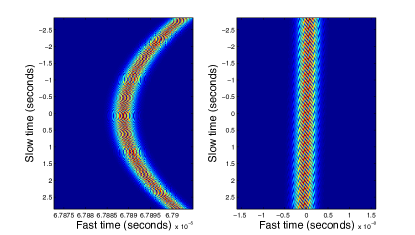
Figure 2: Left: Pulse compressed data $D_{p}(s,t)=f(t-\tau(s,\vec{\boldsymbol{\rho}}))$ from a target at $\vec{\boldsymbol{\rho}}=(0,5,0)$m, recorded by a SAR antenna moving at speed $V=70$ m/s along a linear aperture of $400$ m, at range $L=10$ km from $\vec{\boldsymbol{\rho}}$. Right: Range-compressed data $D_{r}(s,t^{\prime})$ with respect to $\vec{\boldsymbol{\rho}}_{o}=(0,0,0)m$.

The target is at location $\vec{\boldsymbol{\rho}}=(0,5,0)$m and the reference point is at $\vec{\boldsymbol{\rho}}_{o}=(0,0,0)$m. The SAR platform moves at speed $70$m/s along a linear aperture $a=400$m at range $L=10$ km from $\vec{\boldsymbol{\rho}}$. The imaging scene lies on a flat surface at zero altitude. We show in the left plot in Figure 2 the amplitude of the pulse compressed echo as a function of $s$ and $t$. Note that its peak lies on the curve defined by

$$\left(\frac{ct}{2}\right)^{2}=|\vec{\bf r}(s)-\vec{\boldsymbol{\rho}}|^{2}.$$

This curve is a hyperbola because the aperture is linear and the platform moves at constant speed. The right plot in Figure 2 shows the amplitude of the range and pulse compressed echo. Its peak lies on the curve

$$\frac{ct^{\prime}}{2}=|\vec{\bf r}(s)-\vec{\boldsymbol{\rho}}|-|\vec{\bf r}(s)-\vec{\boldsymbol{\rho}}_{o}|,$$

which looks almost as a vertical line segment, because the dependence on the slow time has been approximately removed by the range compression.

We work henceforth with the range and pulse compressed data and drop the prime from the shifted fast time $t^{\prime}$ to simplify the notation. Borrowing terminology from geophysics, we call $D_{r}(s,t)$ the data traces or simply the traces.

2.2 Image formation

A SAR image is formed by superposing the traces over the aperture and back propagating them to the imaging points $\vec{\boldsymbol{\rho}}^{\,\cal I}$ using travel times

$${\cal I}(\vec{\boldsymbol{\rho}}^{\,\cal I}) =\sum_{j=-n/2}^{n/2}D_{r}\left(s_{j},\tau\left(s_{j},\vec{\boldsymbol{\rho}}^{\,\cal I}\right)-\tau(s_{j},\vec{\boldsymbol{\rho}}_{o})\right).$$ (2.6)

The slow time samples $s_{j}$ discretize the interval $[-S(a),S(a)]$ which defines the aperture $a$ along the trajectory of the SAR platform. The sampling $\Delta s$ is uniform and equals the time interval between tho consecutive signal emissions from the antenna. To simplify the notation, we assume that the origin of the slow time corresponds to the center of the aperture. Thus, $n$ is an even integer and

$$2S(a)=n\Delta s.$$

Equation (2.6) is a simplification of the imaging function used in practice, which includes a weight factor that accounts for geometrical spreading. The weight makes a difference only when the aperture is large. We neglect it in this paper because we focus attention on motion estimation, which is necessarily done over small successive sub-apertures. Targets may have complicated trajectories over long data acquisition times, but we can approximate their motion by a uniform translation over short durations $2S(a)$ defining small sub-apertures $a$. The idea is that the speed of translation can be estimated sub-aperture by sub-aperture, and then it can be compensated in the image formation. By compensation we mean that if we seek to image a moving target and we estimate its speed to be $\vec{\bf u}$, we can form an image as

$${\cal I}_{{}_{\vec{\bf u}}}(\vec{\boldsymbol{\rho}}^{\,\cal I})=\sum_{j=-n/2}^{n/2}D_{r}\left(s_{j},\tau\left(s_{j},\vec{\boldsymbol{\rho}}^{\,\cal I}+s_{j}\vec{\bf u}\right)-\tau(s_{j},\vec{\boldsymbol{\rho}}_{o})\right).$$ (2.7)

We repeat the process for successive sub-apertures, and assemble the final image by superposing the results. This superposition requires proper weighting to compensate geometrical spreading effects over long SAR platform trajectories.

Motion estimation and its compensation in imaging works for simple scenes with one or a few targets that move at approximately the same speed. To our knowledge, there is no approach that estimates motion in complex scenes with a single antenna. Moreover, even if a target speed were estimated, the compensation in (2.7) would bring that target in focus but it would blur the others. To address the difficulty of imaging with motion estimation in complex scenes, we propose a data pre-processing step for separating the traces from the stationary targets and the moving ones. If we could achieve such separation, we could carry the motion estimation on the data traces from the moving targets alone. Moreover, we could image the stationary and moving targets separately, and then combine the results to obtain an image of the complex scene.

3 Data separation

We present two complementary approaches for separating traces from stationary and moving targets. They are analyzed in section 4, in simple setups. Here we describe how they work and illustrate the ideas with numerical simulations, for a complex scene named hereafter “Scene 1”. It consists of twenty stationary targets and two moving targets with speeds of $28$m/s and $14$m/s, respectively. We refer to section 5 for details on the setup of the numerical simulations. The traces are displayed in the left plot of Figure 6.

3.1 Travel time transformations and data separation

The basic idea of the first data separation approach is that if we have an estimate $\vec{\boldsymbol{\rho}}^{e}$ of the location $\vec{\boldsymbol{\rho}}$ of a stationary target, we can shift the time $t$ by the travel time $\tau(s,\vec{\boldsymbol{\rho}}^{e})$ to remove approximately the dependence on the slow time $s$ of the trace from that target. Then, we can subtract the trace from the data by exploiting its independence of $s$. To determine $\vec{\boldsymbol{\rho}}^{e}$, we need a preliminary image of the scene. The assumption is that the stationary targets dominate the scene, and therefore they are visible in the preliminary image even in the presence of moving targets. See Figure 3 for an illustration.

Figure 3: Left: The image of the complex Scene 1, with twenty stationary targets and two moving targets. Right: Image of the same stationary scene, and no moving targets. The effect of the moving targets in the left image amounts to two faint streaks.

Let $\mathbb{T}_{+}^{\vec{\boldsymbol{\rho}}^{e}}$ be the map taking the range compressed data $D_{r}(s,t)$ to the data in the transformed coordinates $(s,t+\Delta\tau(s,\vec{\boldsymbol{\rho}}^{e}))$

$$[\mathbb{T}_{+}^{\vec{\boldsymbol{\rho}}^{e}}D_{r}](s,t)=D_{r}(s,t+\Delta\tau(s,\vec{\boldsymbol{\rho}}^{e})),$$ (3.1)

where

$$\Delta\tau(s,\vec{\boldsymbol{\rho}}^{e})=\tau(s,\vec{\boldsymbol{\rho}}^{e})-\tau(s,\vec{\boldsymbol{\rho}}_{o}).$$ (3.2)

Recall that $\vec{\boldsymbol{\rho}}_{o}$ is the reference point in the range compression. To illustrate the effect of the map (3.1), we show on the left in Figure 4 the trace from a target at location $\vec{\boldsymbol{\rho}}\neq\vec{\boldsymbol{\rho}}_{o}$. The plot on the right shows the trace after the travel time transformation (3.1), with the ideal estimate $\vec{\boldsymbol{\rho}}^{e}=\vec{\boldsymbol{\rho}}$. The transformation makes the trace independent of $s$, and thus it can be annihilated by a difference operator in $s$,

$$\mathbb{D}_{s}[\mathbb{T}_{+}^{\vec{\boldsymbol{\rho}}^{e}}D_{r}](s,t)=\frac{1}{\Delta s}\left\{[\mathbb{T}_{+}^{\vec{\boldsymbol{\rho}}^{e}}D_{r}](s+\Delta s,t)-[\mathbb{T}_{+}^{\vec{\boldsymbol{\rho}}^{e}}D_{r}](s,t)\right\}\approx\frac{\partial}{\partial s}[\mathbb{T}_{+}^{\vec{\boldsymbol{\rho}}^{e}}D_{r}](s,t).$$ (3.3)

This is an extension of the ideas proposed in [4, 5] for annihilating echoes from a layered scattering medium. Other annihilation operators than (3.3) may be used, as well. In practice, where noise plays a role, they should be complemented with a smoothing process. We refer to [4, 5] for a detailed analysis of annihilator filters. For the simulations in this paper the annihilator $\mathbb{D}_{s}$ works well, and there is no noise added to the data.

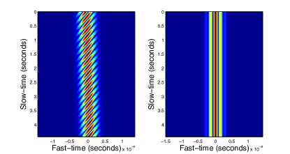
Figure 4: Left: The trace $|D_{r}(s,t)|$ from one stationary target. Right: the traces after the travel time transformation relative to the exact location of the target. Note that there is no dependence on $s$ after the transformation.

After taking the derivative, we map the traces back to the $(s,t)$ coordinates using the travel time transformation $\mathbb{T}_{-}^{\vec{\boldsymbol{\rho}}^{e}}$. The data filter is a linear operator denoted by $Q^{\vec{\boldsymbol{\rho}}^{e}}$, given by composition of $\mathbb{T}_{+}^{\vec{\boldsymbol{\rho}}^{e}}$, $\mathbb{D}_{s}$ and $\mathbb{T}_{-}^{\vec{\boldsymbol{\rho}}^{e}}$,

$$\left[\mathcal{Q}^{\vec{\boldsymbol{\rho}}^{e}}D_{r}\right](s,t)=\left[\mathbb{T}_{-}^{\vec{\boldsymbol{\rho}}^{e}}\mathbb{D}_{s}\mathbb{T}_{+}^{\vec{\boldsymbol{\rho}}^{e}}D_{r}\right](s,t)=\left[\mathbb{D}_{s}D_{r}(s,t^{\prime}+\Delta\tau(s,\vec{\boldsymbol{\rho}}^{e}))\right]_{t^{\prime}=t-\Delta\tau(s,\vec{\boldsymbol{\rho}}^{e})}.$$ (3.4)

We demonstrate in Figure 5 the travel-time transformations and annihilation steps for a scene with one stationary and one moving target. Note that the trace from the stationary target located at $\vec{\boldsymbol{\rho}}$ is completely removed by the mapping $Q^{\vec{\boldsymbol{\rho}}^{e}}$, because $\vec{\boldsymbol{\rho}}^{e}=\vec{\boldsymbol{\rho}}$.

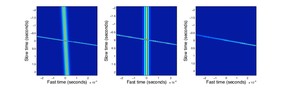
Figure 5: Left: The traces $D_{r}(s,t)$ for a scene with one stationary target at location $\vec{\boldsymbol{\rho}}$ and a moving one at $28$m/s. Middle: The traces after the travel time transformation $[\mathbb{T}_{+}^{\vec{\boldsymbol{\rho}}}D_{r}](s,t)$. Right: The filtered traces $[\mathcal{Q}^{\vec{\boldsymbol{\rho}}^{e}}D_{r}](s,t)$.

If there are $N$ stationary targets in the scene, we can subtract their traces from the data one by one, by iterating the procedure above. Let $\vec{\boldsymbol{\rho}}_{j}^{e}$ be the estimated locations of the targets, with $j=1,\ldots,N$. The data filter $\mathcal{Q}$ is the composition of the linear operators (3.4),

$$\left[\mathcal{Q}D_{r}\right](s,t)=\left[\mathcal{Q}^{\vec{\boldsymbol{\rho}}_{N}^{e}}\circ\mathcal{Q}^{\vec{\boldsymbol{\rho}}_{N-1}^{e}}\circ\ldots\circ\mathcal{Q}^{\vec{\boldsymbol{\rho}}_{1}^{e}}D_{r}\right](s,t).$$ (3.5)

The estimates $\vec{\boldsymbol{\rho}}_{j}^{e}$ are not exact in practice, but the filter (3.4) is robust with respect to the estimation errors. We show this in section 4, where we present a brief analysis of the filters. In fact, our simulations show that it is typical that one application of $\mathcal{Q}^{\vec{\boldsymbol{\rho}}^{e}}$ removes at once the traces from all the stationary targets located near $\vec{\boldsymbol{\rho}}^{e}$. Thus, the needed number of iterations in (3.5) may be much smaller than the number of stationary targets in practice.

Because antennas measure discrete samples of the data $D_{r}(s,t)$, we need to use interpolation when making the travel-time transformations. We do so by implementing the travel-time transformations as phase modulations in the frequency domain

$$\left[\mathbb{T}_{+}^{\vec{\boldsymbol{\rho}}^{e}}D_{r}\right](s,t)=\frac{1}{2\pi}\int d\omega\ \widehat{D}_{r}(s,\omega)e^{-i\omega(t+\Delta\tau(s,\vec{\boldsymbol{\rho}}))},$$ (3.6)

where

$$\widehat{D}_{r}(s,\omega)=\int dt\ e^{i\omega t}D_{r}(s,t).$$

We implement (3.6) in the discrete setting using the fast Fourier transform.

3.2 Data separation with robust PCA

We introduced recently in [2] a method for separating the traces from stationary and moving targets using robust principal component analysis (PCA). We review here the data separation method, and give some details of its analysis in section 4.

The robust PCA method was introduced and analyzed in [7]. It decomposes a matrix ${\cal M}$ into a low rank matrix ${\cal L}$ and a sparse matrix ${\cal S}$. In our context, the entries in ${\cal M}$ are the samples of the traces

$${\cal M}_{j\ell}=D_{r}(s_{j},t_{\ell}),$$ (3.7)

where

$$s_{j}=j\Delta s,\quad j=-n/2,\ldots,n/2,\quad 2S(a)=n\Delta s,$$ (3.8)

and

$$t_{\ell}=\ell\Delta s,\quad\ell=-m/2,\ldots,m/2,\quad\Delta s=m\Delta t.$$ (3.9)

The sampling is at uniform intervals $\Delta s$ and $\Delta t$, determined in practice by the SAR antenna system. To simplify the notation, we take the origin of $s$ at the center of the aperture, and the origin of $t$ in the middle of the interval $\Delta s$ between two consecutive signal emissions.

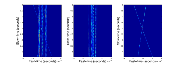
Figure 6: Left: The matrix ${\cal M}$ of the sampled traces from Scene 1. Middle: The matrix ${\cal L}$ consisting of the traces from the stationary targets in Scene 1. Right: The matrix ${\cal S}$ consisting of the traces from the moving targets in Scene 1.

To explain why we can use robust PCA for the data separation, consider the matrix ${\cal M}$ of sampled traces for Scene 1. We display it in the left plot of Figure 6. The traces that appear almost vertical correspond to the stationary targets. This is because these targets are not too far from the reference point $\vec{\boldsymbol{\rho}}_{o}$, and the range compression removes most of their $s$ dependence. We expect that these traces form a low rank matrix ${\cal L}$. We display them in the middle plot of Figure 6. The range compression does not remove the slow time dependence of the traces from the moving targets, so they appear sloped in Figure 6. They form a high rank but sparse matrix ${\cal S}$, shown in the right plot of Figure 6.

The robust PCA method is designed to separate ${\cal L}$ from ${\cal S}$ in ${\cal M}={\cal L}+{\cal S}.$ It does so by solving an optimization problem called principle component pursuit [7]

$$\min_{{\cal L},{\cal S}\in\mathbb{R}^{n+1\times m+1}}\|{\cal L}\|_{*}+\eta\|{\cal S}\|_{1},\quad\mbox{subject to}\quad{\cal L}+{\cal S}={\cal M}.$$ (3.10)

Here $\|{\cal L}\|_{*}$ is the nuclear norm of ${\cal L}$, the sum of the singular values of ${\cal L}$, $\|{\cal S}\|_{1}$ is the matrix 1-norm of ${\cal S}$ and

$$\eta=\frac{1}{\sqrt{\max\{n+1,m+1\}}}.$$ (3.11)

The optimization (3.10) can be applied to any matrix ${\cal M}$. But it is shown in [7] that if ${\cal M}$ is a matrix with a low rank part ${\cal L}$ and a high rank sparse part ${\cal S}$, then the algorithm recovers exactly ${\cal L}$ and ${\cal S}$. We refer to [7] for sufficient (not necessary) conditions satisfied by ${\cal M}$, so that it can be succesfully decomposed by principle component pursuit.

Robust PCA is well suited for our purpose, but it cannot be applied as a black box to the matrix of traces. We need to complement it with properly calibrated data windowing. To illustrate why, we present two examples.

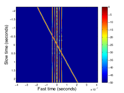
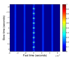
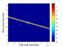
Figure 7: Separation of traces from the scene in Example 1. From left to right we show the matrix ${\cal M}$ of traces, the low rank ${\cal L}$, and sparse ${\cal S}$ components obtained with robust PCA. Top row: robust PCA applied to the entire data matrix ${\cal M}$. Bottom row: robust PCA applied to a windowed ${\cal M}$. In each plot the matrices are normalized by the largest value of $|{\cal M}|$. The sparse components shown in the right column are plotted in (decibel) dB scale to make the contrast more visible.

Example 1: The first example considers a scene with one moving target and seven stationary ones. The moving target is at location $(0,0,0)$m at time $s=0$, corresponding to the center of the aperture, and velocity $\vec{\bf u}=28/\sqrt{2}(1,1,0)$m/s. The stationary scatterers are located at $(0,0,0)$m, $(\pm 5,0,0)$m, $(0,\pm 5,0)$m, and $(\pm 10,0,0)$m. in the imaging region. The reference point is $\vec{\boldsymbol{\rho}}_{o}=(0,0,0)$m.

When we apply the robust PCA method to the matrix of traces shown in the top left plot in Figure 7, we obtain the “low rank”and “sparse” parts shown in the top middle and top right plots. We note from the right plot that the “sparse” component contains the trace from the moving target but also remnants of the traces from the stationary targets. The data separation is not successful because the matrix ${\cal M}$ is sparse to begin with.

However, if we apply robust PCA to the matrix of traces in a smaller fast-time window, we get a successful separation. This is shown in the bottom row of Figure 7. The windowed ${\cal M}$ has a much larger number of non-zero entries relative to its size, and robust PCA separates the traces from the moving target and the stationary ones.

Example 2: The second example considers a scene with thirty stationary scatterers and the same moving target as in example 1. The matrix ${\cal M}$ of traces is displayed in Figure 8. The results with robust PCA applied to the entire ${\cal M}$ are in the top row of Figure 9. Again, we see that the “sparse” part contains remnants of the traces from the stationary targets. This is not because ${\cal M}$ is sparse, as was the case in example 1, but because the traces from the stationary targets do not form a matrix of sufficiently low rank. When we window ${\cal M}$, we work with a few nearby traces at a time. These traces are similar to each other so they form a low rank matrix that can be separated with robust PCA. The final result is given by the concatenation of the matrices in each window. It is shown in the bottom row of Figure 9.

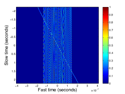
Figure 8: Matrix ${\cal M}$ of traces from the scene in Example 2.

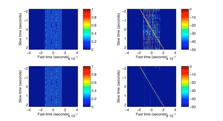
Figure 9: Robust PCA separation of traces from a scene with thirty stationary targets and one moving target. The top row of plots shows the results with robust PCA applied to the entire data matrix in Figure 8. The low rank and sparse components are shown on the left and right, respectively. The bottom row of plots shows the results with robust PCA applied to successive small time windows of the data. The sparse components shown in the right column are plotted in dB scale to make the contrast more visible.

These two examples show that windowing is a key step to successful data separation with robust PCA. To choose appropriate window sizes, it is necessary to understand how the rank and sparsity of the data matrix ${\cal M}$ depend on the location and density of the stationary targets, and on the velocity of moving targets. This is addressed in the analysis of [2], which we review in section 4.4.

3.3 Discussion

We use numerical simulations for Scene 1 to compare the two methods described in sections 3.1 and 3.2. The results are in Figures 10 and 11.

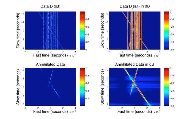
Figure 10: Annihilation with the filter (3.5) of the stationary target traces from Scene 1. Top: the matrix of traces. Bottom: the filtered traces. In each plot we show absolute values normalized by the largest value of $|{\cal M}|$. The right column is the left column plotted in dB scale.

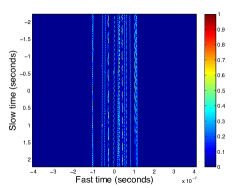
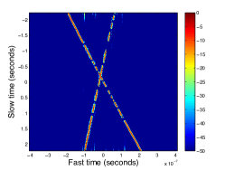
Figure 11: Trace separation with robust PCA for Scene 1. The low rank part ${\cal L}$ is shown on the left and the sparse part ${\cal S}$ is shown on the right. In each plot we show absolute values normalized by the largest value of $|{\cal M}|$. The sparse part is plotted in dB scale.

The first method uses the filter $\mathcal{Q}$ defined in (3.5) to annihilate the traces from the stationary targets. We see from Figure 10 that this is accomplished, but the filter removes some parts of the traces from the moving targets as well. All our numerical simulations show that $\mathcal{Q}$ separates nicely the traces from the moving targets if the scene does not have too many stationary targets at almost the same range. Otherwise, it also removes parts of the traces from the moving targets.

The data separation with the robust PCA approach is better, as seen in Figure 11. This method is more sophisticated than the other, because it involves careful windowing of the traces, but it works better for complex scenes that are not too large. Robust PCA relies heavily on range compression removing most of the slow-time dependence of the traces from the stationary targets. But for extended scenes there is no single reference point $\vec{\boldsymbol{\rho}}_{o}$ that accomplishes this task, and data separation with robust PCA deteriorates. The filter (3.5) still works for extended scenes, because the travel time transformations in (3.4) are relative to the location of the targets that we wish to annihilate, and not some arbitrary reference point.

In principle, we can use a combination of the two approaches to improve the data separation with robust PCA for extended scenes. The idea is to begin with a preliminary image and identify roughly the stationary targets to be separated from the scene. Then we can window the image around groups of such targets and work with one subscene at a time. It is important to observe here that if the aperture is not too large, as is the case in motion estimation, the image is approximately the Fourier transform of the data with a phase correction. See for example [3] for a detailed explanation of this fact. Thus, we can obtain approximately the traces from the smaller subscene by Fourier transforming the windowed image. To separate these traces, we can apply the travel time transformation (3.1) with a reference point $\vec{\boldsymbol{\rho}}^{e}$ in the subscene, followed by the robust PCA approach as described above.

3.4 Velocity estimation and separation of traces from multiple moving targets

Let us assume in this section that the traces from the stationary targets have been removed, and denote by the same $D_{r}(s,t)$ the traces from the moving targets. Since there may be multiple moving targets, we would like to separate these traces further, based on differences between the target velocities. We can do so by extending the annihilation filters described in section 3.1, as we explain next.

We need a key observation, shown with analysis in section 4. The slope of the trace from a moving target is determined approximately by its speed along the unit vector

$$\vec{\bf m}_{o}=\frac{\vec{\bf r}(0)-\vec{\boldsymbol{\rho}}_{o}}{|\vec{\bf r}(0)-\vec{\boldsymbol{\rho}}_{o}|},$$ (3.12)

pointing from the SAR platform location $\vec{\bf r}(0)$ at the middle of the aperture to the reference point $\vec{\boldsymbol{\rho}}_{o}$ in the imaging scene. Moreover, the curvature of the trace is determined by the speed projected on the plane orthogonal to $\vec{\bf m}_{o}$.

Because we assume a flat imaging surface, the target speed $\vec{\bf u}$ is a vector in the horizontal plane

$$\vec{\bf u}=({\bf u},0),\quad{\bf u}\in\mathbb{R}^{2}.$$ (3.13)

We parametrize it by the range velocity $u$ and the cross-range velocity $u_{\perp}$. The range velocity is

$$u=\vec{\bf u}\cdot\vec{\bf m}_{o}={\bf u}\cdot{\bf m}_{o},$$ (3.14)

where ${\bf m}_{o}$ is the projection of $\vec{{\bf m}}_{o}$ on the imaging plane. The cross-range velocity is defined by

$$u_{\perp}=\vec{\bf t}\cdot\mathbb{P}_{o}\vec{\bf u}={\bf u}\cdot{\bf t}-u\,\vec{{\bf m}}_{o}\cdot\vec{{\bf t}}(0),$$ (3.15)

where $\mathbb{P}_{o}$ is the orthogonal projection

$$\mathbb{P}_{o}=I-\vec{{\bf m}}_{o}\vec{{\bf m}}_{o}^{T},$$ (3.16)

and $\vec{\bf t}$ is the unit vector tangent to the SAR platform trajectory, at the center $\vec{\bf r}(0)$ of the aperture. Note that in many setups $\vec{{\bf m}}_{o}$ and $\vec{{\bf t}}$ are almost orthogonal, so $u_{\perp}$ is approximately the target speed along the vector ${\bf t}$, the projection of $\vec{{\bf t}}$ on the imaging plane.

Next, we define the transformation mapping $\mathbb{T}^{\vec{\bf u}^{e},\vec{\boldsymbol{\rho}}^{e}}_{+}$, the generalization of (3.1),

$$\left[\mathbb{T}^{\vec{\bf u}^{e},\vec{\boldsymbol{\rho}}^{e}}_{+}D_{r}\right](s,t)=D_{r}\left(s,t+\Delta\tau(s,\vec{\boldsymbol{\rho}}^{e}+s\vec{\bf u}^{e})\right),$$ (3.17)

with $\Delta\tau$ given in (3.2). Here $\vec{\boldsymbol{\rho}}^{e}$ is the estimated location of the moving target at the origin of the slow time, and $\vec{\bf u}^{e}$ is the estimated velocity. If the line segment

$$\vec{\boldsymbol{\rho}}^{e}+s\vec{\bf u}^{e},\quad s\in[-S(a),S(a)],$$

is close to the target trajectory, then the transformation (3.17) removes approximately the dependence of its trace on the slow time. Thus, we can subtract it from the other traces using the same difference operator $\mathbb{D}_{s}$. The annihilation filter is the generalization of (3.4),

$$\left[\mathcal{Q}^{\vec{\bf u}^{e},\vec{\boldsymbol{\rho}}^{e}}D_{r}\right](s,t) = \left[\mathbb{T}^{\vec{\bf u}^{e},\vec{\boldsymbol{\rho}}^{e}}_{-}\mathbb{D}_{s}\mathbb{T}^{\vec{\bf u}^{e},\vec{\boldsymbol{\rho}}^{e}}_{+}D_{r}\right](s,t)$$ (3.18)

$$= \left[\mathbb{D}_{s}D_{r}\left(s,t^{\prime}+\Delta\tau(s,\vec{\boldsymbol{\rho}}^{e}+s\vec{\bf u}^{e})\right)\right]_{t^{\prime}=t-\Delta\tau(s,\vec{\boldsymbol{\rho}}^{e}+s\vec{\bf u}^{e})},$$

where the mapping $\mathbb{T}^{\vec{\bf u}^{e},\vec{\boldsymbol{\rho}}^{e}}_{-}$ undoes the travel time transformation. Additionally we can apply robust PCA to $\left[\mathbb{T}^{\vec{\bf u}^{e},\vec{\boldsymbol{\rho}}^{e}}_{+}D_{r}\right](s,t)$. This should result in the low rank matrix containing the trace corresponding to the moving target with velocity $\vec{\boldsymbol{\rho}}^{e}$ and the sparse matrix containing the rest of the moving target traces.

The implementation of (3.17) and (3.18) requires the estimates $\vec{\boldsymbol{\rho}}^{e}$ and $\vec{\bf u}^{e}$. There are two scenarios. The first assumes that we know $\vec{\boldsymbol{\rho}}^{e}$ from tracking the target in previous sub-apertures, and seeks only $\vec{\bf u}^{e}$. The second seeks both $\vec{\boldsymbol{\rho}}^{e}$ and $\vec{\bf u}^{e}$. In either case, the estimation begins with that of the range velocity, which controls the slope of the trace. Then, we can estimate $\vec{\boldsymbol{\rho}}^{e}$ if we need to, and the cross-range speed $u_{\perp}^{e}$.

We estimate $u^{e}$ as the maximizer of the objective function

$$g(u)=\max_{-m/2\leq\ell\leq m/2}\sum_{j=-n/2}^{n/2}\left|\left[\mathbb{T}^{\vec{\bf u},\vec{\boldsymbol{\rho}}^{e}}_{+}D_{r}\right](s_{j},t_{\ell})\right|,\quad\vec{\bf u}=u\,({\bf m}_{o},0).$$ (3.19)

The idea is that when $u^{e}$ is close to the range speed of the target, the transformation $\mathbb{T}^{\vec{\bf u},\vec{\boldsymbol{\rho}}^{e}}_{+}$ makes the trace an approximate line segment, and when we sum it over $s$, we get a peak around some fast time $t_{\ell}$, for $|\ell|\leq m/2$. If we do not know $\vec{\boldsymbol{\rho}}^{e}$, we can set it equal to $\vec{\boldsymbol{\rho}}_{o}$ in (3.19). Then, we can form an image ${\cal I}_{\vec{\bf u}^{e}}(\vec{\boldsymbol{\rho}}^{\,\cal I})$ using (2.7) with $\vec{\bf u}^{e}=u^{e}({\bf m}_{o},0)$, and estimate $\vec{\boldsymbol{\rho}}^{e}$ from there. The motion compensation in (2.7) brings the moving target approximately in focus, and this is why we expect to be able to estimate its location from the image.

Once we have estimated $u^{e}$ and $\vec{\boldsymbol{\rho}}^{e}$, we seek the cross-range speed $u_{\perp}^{e}$ as the minimizer of the objective function

$$g_{\perp}(u_{\perp};u^{e},\vec{\boldsymbol{\rho}}^{e})=\sum_{\ell=-m/2}^{m/2}\sum_{j=-n/2}^{n/2}\left|\mathbb{D}^{2}_{s}\left[\mathbb{T}^{\vec{\bf u},\vec{\boldsymbol{\rho}}^{e}}_{+}D_{r}\right](s_{j},t_{\ell})\right|,$$ (3.20)

which quantifies the curvature of the trace. Here $\mathbb{D}^{2}_{s}$ approximates the second derivative in $s$, and $\vec{\bf u}=({\bf u},0)$ is defined by

$${\bf u}\cdot{\bf m}_{o}=u^{e},\quad{\bf u}\cdot{\bf t}(0)=u_{\perp}+u^{e}\vec{{\bf m}}_{o}\cdot\vec{{\bf t}}(0).$$ (3.21)

Because $u_{\perp}$ has a weaker effect on the traces than $u$, it is more difficult to estimate it. Even if there is no noise, the estimation is sensitive to remnants of the traces from the stationary targets that have not been perfectly annihilated, the traces from the other moving targets, and the discrete sampling of the data. If we took the maximum over $\ell$ of the sum

$${\cal F}(u_{\perp},\ell)=\sum_{j=-n/2}^{n/2}\left|\left[\mathbb{D}^{2}_{s}\mathbb{T}^{\vec{\bf u},\vec{\boldsymbol{\rho}}^{e}}_{+}D_{r}\right](s_{j},t_{\ell})\right|$$

as we did in the objective function (3.19), we would seek a saddle point of ${\cal F}$ to estimate $u_{\perp}$. That is to say, we would minimize with respect to $u_{\perp}$ and maximize with respect to $\ell$. Our numerical simulations show that such an estimation is not robust. To stabilize it, we sum over $\ell$ in (3.20) and reduce the problem to that of minimizing in $u_{\perp}$.

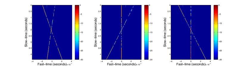
Figure 12: Left: The traces from the two moving targets in Scene 1. Middle and right: The transformed traces $\mathbb{T}^{\vec{\bf u},\vec{\boldsymbol{\rho}}}_{+}D_{r}(s,t)$ for the first and second target.

As an illustration, we present the results for Scene 1. Figure 12 displays $\mathbb{T}^{\vec{\bf u},\vec{\boldsymbol{\rho}}}_{+}D_{r}(s,t)$ using the true locations $\vec{\boldsymbol{\rho}}$ and velocities $\vec{\bf u}$ for the two moving targets. Note how after the transformation the traces become vertical line segments. If we were to search for the range speed $u^{e}$ without annihilating the traces of the stationary targets, we would get the objective function $g(u)$ plotted on the left in Figure 13. The prominent peak of $g$ is at speed $u=0$, because the stationary targets dominate the scene. The smaller peaks are due to the two moving targets. When we compute the objective function $g(u)$ with the traces from the moving targets alone, we get two large peaks, at the range speeds of the targets. The speed in (3.17) is $\vec{\bf u}=u^{e}({\bf m}_{o},0)$, with $u^{e}$ estimated from the first and second peak of $g(u)$, respectively.

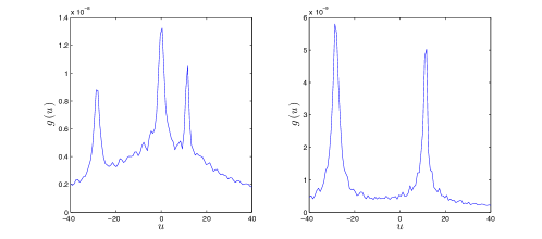
Figure 13: The objective function $g(u)$ using the traces from the entire Scene 1 (left) and the traces from the moving targets in Scene 1 (right).

Recall that the cross-range speed $u_{\perp}$ has a weaker effect on the traces than the range speed, it determines only their curvature. We illustrate this in the top right plot of Figure 14, where we zoom around the trace of one target, rotated with transformation (3.17) at the estimated range speed $u^{e}({\bf m}_{o},0)$. The bottom row in Figure 14 shows the traces transformed with (3.17), after the cross-range speed correction. The trace is now straightened, as seen in the bottom right plot. The objective function (3.20) is shown in the middle and right plots of Figure 15. We plot it for the two range speeds, the peaks of $g$ shown on the left. The function $g_{\perp}$ has minima at the cross-range speeds of the two targets.

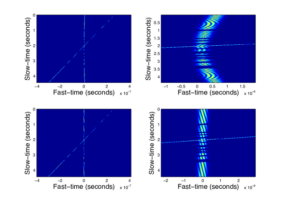
Figure 14: Top row: The traces after the travel time transformation (3.17) at the estimated range speed of one target. Bottom row: The traces after the travel time transformation (3.17) with the estimated cross-range correction of the speed. The right column is a zoom of the left column.

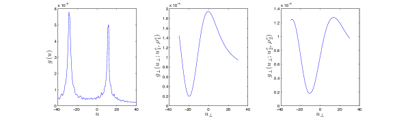
Figure 15: Left: The objective function $g$. Middle and right: The objective function $g_{\perp}$ for the estimated range speeds of the two targets in Scene 1. The minima of $g_{\perp}$ are the estimates of $u_{\perp}$.

4 Analysis

In this section we give a brief analysis of our data separation approaches. The analysis is for simple scenes, but the methods work in complex scenes, as shown already in the previous section. More numerical results are in section 5. We begin with the data model and the scaling regime. Then, we analyze the annihilation filters defined in section 3.1. The analysis extends to the filters described in section 3.4, once we explain how the target velocity affects the traces. We end the section with a brief review of the analysis in [2] of the data separation with robust PCA.

4.1 Scaling Regime

We illustrate our scaling regime using the GOTCHA Volumetric SAR data set. The relevant scales are the central frequency $\nu_{o}$, the bandwidth $B$, the typical range $L$ from the SAR platform to the targets, the aperture $a$, the magnitude $|\vec{\bf u}|$ of the velocity of the targets, the speed $V$ of the SAR platform and $R^{{\cal I}}$, the diameter of the imaging set ${\cal J}^{{}^{\cal I}}$. We let $L=|\vec{\bf r}(0)-\vec{\boldsymbol{\rho}}_{o}|$, and assume that

$$B\ll\nu_{o},\quad a\ll L,\quad R^{{}^{\cal I}}\ll L.$$ (4.1)

We also suppose that the target speed is smaller than that of the SAR platform

$$|{\bf u}|<V.$$ (4.2)

The GOTCHA parameters satisfy these assumptions:

• The central frequency is $\nu_{0}=9.6$GHz and the bandwidth is $B=622$MHz.

• The SAR platform trajectory is circular, at height $H=7.3$ km, with radius $R=7.1$km and thus $L\approx 10$km. We consider sub-apertures of one circular degree, which corresponds to $a=124$m, and image in domains of radius $R^{{}^{\cal I}}\leq 50$m.

• The platform speed is $V=70$m/s and the targets move with velocities $|\vec{\bf u}|\leq 28$m/s.

• The pulse repetition rate is $117$ per degree, which means that a pulse is sent every $1.05$m, and $\Delta s=0.015$s.

For a stationary target, we obtain from basic resolution theory [3, 18] that the range resolution is $c/B=48$cm, and the cross range resolution is $\lambda_{0}L/a=2.5$m, with one degree aperture $a$ and central wavelength $\lambda_{0}=3$cm.

4.2 Data model

We use a simple data model that approximates the scatterers by point targets in the horizontal plane and neglects multiple scattering between them. We also suppose that the target trajectories can be approximated locally, for the slow time interval defining a single sub-aperture, by the straight line segment

$$\vec{\boldsymbol{\rho}}(s)=\vec{\boldsymbol{\rho}}(0)+s\vec{\bf u},$$

with constant speed $\vec{\bf u}=({\bf u},0)$, and ${\bf u}\in\mathbb{R}^{2}$. The traces are modeled by

$$D_{r}(s,t)\approx\sum_{q=1}^{N}\frac{\sigma_{q}(\omega_{o})}{(4\pi|\vec{\bf r}(s)-\vec{\boldsymbol{\rho}}_{q}(s)|)^{2}}f_{p}(t-(\tau(s,\vec{\boldsymbol{\rho}}_{q}(s))-\tau(s,\vec{\boldsymbol{\rho}}_{o}))),$$ (4.3)

where $N$ is the number of targets. They are located at $\vec{\boldsymbol{\rho}}_{q}(s)$ and with reflectivity $\sigma_{q}(\omega_{o})$, for $q=1,\ldots,N$. The model neglects the displacement of the targets during the round trip travel time. This is justified in radar applications because the waves travel at the speed of light which is several orders of magnitude larger than the speed of the targets. We refer to [3] for a derivation of model (4.3) in the scaling regime described above. We simplify it further by approximating the amplitude factors

$$\frac{1}{4\pi|\vec{\bf r}(s)-\vec{\boldsymbol{\rho}}_{q}(s)|}\approx\frac{1}{4\pi L},$$

and assuming that the targets have the same reflectivity

$$\sigma_{q}(\omega_{o})=\sigma(\omega_{o}),\quad q=1,\ldots,N.$$

The model of the traces becomes

$$D_{r}(s,t)\approx\frac{\sigma(\omega_{o})}{(4\pi L)^{2}}\mathcal{M}(s,t),$$ (4.4)

with

$$\mathcal{M}(s,t)=\sum_{q=1}^{N}f_{p}(t-\Delta\tau(s,\vec{\boldsymbol{\rho}}_{q}(s))),$$ (4.5)

and $\Delta\tau$ given in (3.2). Thus, the traces are approximately, up to a multiplicative constant, equal to the matrix $\{{\cal M}(s_{j},t_{\ell})\}$, for $j=-n/2,\ldots,N/2$ and $\ell=-m/2,\ldots,m/2$. We neglect the multiplicative constant hereafter, and call ${\cal M}$ the matrix of traces.

We could take any pulse $f_{p}$ in (4.5), but to simplify the calculations in the remainder of the section, we assume it Gaussian, modulated by a cosine at the central frequency,

$$f_{p}(t)=\cos(\omega_{o}t)e^{-B^{2}t^{2}/2}.$$ (4.6)

4.3 The annihilation filter

Recall that the filter $\mathcal{Q}^{\vec{\boldsymbol{\rho}}^{e}}$ defined by (3.4) is a linear operator. Because we model the traces (4.5) as a superposition of pulses $f_{p}$ delayed by the travel times to the targets, we can study the effect of $\mathcal{Q}^{\vec{\boldsymbol{\rho}}^{e}}$ on one trace at a time.

Consider the trace from a stationary or moving target at location $\vec{\boldsymbol{\rho}}_{j}(s)$, for some integer $j$ satisfying $1\leq j\leq N$, and denote it by

$${\cal M}^{j}(s,t)=f_{p}(t-\Delta\tau(s,\vec{\boldsymbol{\rho}}_{j}(s))).$$ (4.7)

The transformation $\mathbb{T}_{+}^{\vec{\boldsymbol{\rho}}^{e}}$ defined in (3.1) maps the trace to

$$\left[\mathbb{T}_{+}^{\vec{\boldsymbol{\rho}}^{e}}{\cal M}^{j}\right](s,t)=f_{p}\left(t+\Delta\tau(s,\vec{\boldsymbol{\rho}}^{e})-\Delta\tau(s,\vec{\boldsymbol{\rho}}_{j}s))\right),$$ (4.8)

and then we filter it with the difference operator $\mathbb{D}_{s}$,

$$\mathbb{D}_{s}\left[\mathbb{T}_{+}^{\vec{\boldsymbol{\rho}}^{e}}{\cal M}^{j}\right](s,t)\approx A(s,\vec{\boldsymbol{\rho}}_{j}(s),\vec{\boldsymbol{\rho}}^{e})f^{\prime}_{p}\left(t+\Delta\tau(s,\vec{\boldsymbol{\rho}}^{e})-\Delta\tau(s,\vec{\boldsymbol{\rho}}_{j}(s))\right).$$ (4.9)

Here we approximate the finite difference by the derivative in $s$, denote by $f_{p}^{\prime}$ the derivative of the pulse, and let $A$ be the “annihilation factor”

$$A(s,\vec{\boldsymbol{\rho}}_{j}(s),\vec{\boldsymbol{\rho}}^{e})=\frac{d}{ds}\left[\tau(s,\vec{\boldsymbol{\rho}}_{j}(s))-\tau(s,\vec{\boldsymbol{\rho}}^{e})\right].$$ (4.10)

Using the scaling assumptions (4.1-4.2), we obtain after a straightforward calculation that

$$\frac{d}{ds}\left[\tau(s,\vec{\boldsymbol{\rho}}_{j}(s))-\tau(s,\vec{\boldsymbol{\rho}}^{e})\right]=\frac{2}{c}\left[-\vec{\bf u}\cdot\vec{{\bf m}}_{e}+\frac{(V\vec{{\bf t}}-\vec{\bf u})\cdot\mathbb{P}_{e}\Delta\vec{\boldsymbol{\rho}}_{j}}{L}-s\frac{(2V\vec{{\bf t}}-\vec{\bf u})\cdot\mathbb{P}_{e}\vec{\bf u}}{L}\right]+$$

$$O\left(\frac{au_{\perp}}{cL}\right)+O\left(\frac{aVR^{\cal I}}{cL^{2}}\right),\quad$$ (4.11)

where

$$\Delta\vec{\boldsymbol{\rho}}_{j}=\vec{\boldsymbol{\rho}}_{j}(0)-\vec{\boldsymbol{\rho}}^{e},\quad\vec{{\bf m}}_{e}=\frac{\vec{\bf r}(0)-\vec{\boldsymbol{\rho}}^{e}}{|\vec{\bf r}(0)-\vec{\boldsymbol{\rho}}^{e}|},\quad\mathbb{P}_{e}=I-\vec{{\bf m}}_{e}\vec{{\bf m}}_{e}^{T}.$$

The annihilation factor of a stationary target is given by

$$A(s,\vec{\boldsymbol{\rho}}_{j},\vec{\boldsymbol{\rho}}^{e})=\frac{2V}{c}\frac{\vec{{\bf t}}\cdot\mathbb{P}_{e}\Delta\vec{\boldsymbol{\rho}}_{j}}{L}+O\left(\frac{aVR^{\cal I}}{cL^{2}}\right).$$ (4.12)

It is approximately linear in the cross-range component of the error $\Delta\vec{\boldsymbol{\rho}}^{e}$ of the estimated location of the target. For a moving target the factor is

$$A(s,\vec{\boldsymbol{\rho}}_{j}(s),\vec{\boldsymbol{\rho}}^{e})\approx\frac{2V}{c}\left[\frac{\vec{{\bf t}}\cdot\mathbb{P}_{e}\Delta\vec{\boldsymbol{\rho}}_{j}}{L}-\frac{u}{V}-2\frac{Vs}{L}\frac{u_{\perp}}{V}\right]+O\left(\frac{au_{\perp}}{cL}\right)+O\left(\frac{aVR^{\cal I}}{cL^{2}}\right).$$ (4.13)

It is much larger than (4.12) for stationary targets that are in the vicinity of $\vec{\boldsymbol{\rho}}^{e}$, and satisfy the condition

$$|\Delta\vec{\boldsymbol{\rho}}_{j}|\ll L\left[O\left(\frac{u}{V}\right)+O\left(\frac{a}{L}\frac{u_{\perp}}{V}\right)\right].$$ (4.14)

Consequently, the filter $\mathcal{Q}^{\vec{\boldsymbol{\rho}}^{e}}$ defined by (3.4) emphasizes the traces from the moving targets and suppresses the traces from the stationary targets near $\vec{\boldsymbol{\rho}}^{e}$, as stated in section 3.1.

Remark 1

In the GOTCHA regime, and for one degree apertures as described in section 4.1, the cross-range resolution of a preliminary image is approximately $2.5$m. Thus, we can assume that for the target that we wish to annihilate $|\Delta\vec{\boldsymbol{\rho}}_{j}|\approx 2.5$m, and condition (4.14) is satisfied for targets moving at range speed that exceeds $0.2$m/s.

Note also from (4.11), with $\vec{\boldsymbol{\rho}}^{e}$ replaced by $\vec{\boldsymbol{\rho}}_{o}$, that the slope of the trace is approximately given by the range speed $u=\vec{\bf u}\cdot\vec{{\bf m}}_{o}$, as assumed in section 3.4, as long as

$$u\gg V\frac{\vec{{\bf t}}\cdot\mathbb{P}_{o}\Delta\vec{\boldsymbol{\rho}}_{j}}{L}\sim V\frac{R^{{\cal I}}}{L}.$$

If the target is a slower mover, than its trace looks similar to that of a stationary target and it cannot be separated. The curvature of the trace is determined by the cross-range velocity of the target, as seen from the third term in the right hand side of equation (4.11).

4.4 Analysis of data separation with robust PCA

In this section we review briefly from [2] the analysis of the rank of the matrix of traces for simple scenes. The goal is to show that indeed, traces from stationary targets should be expected to give a low rank contribution whereas those from the moving targets should give a high rank contribution. This is the key assumption in the data separation approach described in section 3.2.

4.4.1 One target

We begin with the case of one target at location $\vec{\boldsymbol{\rho}}(s)=(\boldsymbol{\rho}(s),0)$. It moves at constant speed $\vec{\bf u}=({\bf u},0)$ over the slow time interval $|s|\leq S(a)$, so we can write that

$$\vec{\boldsymbol{\rho}}(s)=\vec{\boldsymbol{\rho}}+s\,\vec{{\bf u}},\quad|s|\leq S(a),$$ (4.15)

where

$$\vec{\boldsymbol{\rho}}=\vec{\boldsymbol{\rho}}(0).$$

The matrix denoted by ${\cal M}$ is defined by the discrete samples of

$$\mathcal{M}(s,t)=\cos\left[\omega_{o}(t-\Delta\tau(s,\vec{\boldsymbol{\rho}}(s)))\right]\exp\left[-\frac{B^{2}}{2}(t-\Delta\tau(s,\vec{\boldsymbol{\rho}}(s)))^{2}\right],$$ (4.16)

where $\Delta\tau$ is defined by (3.2), and we used the pulse (4.6). The rank of ${\cal M}$ is the same as that of the symmetric, square matrix $\mathcal{Y}\in\mathbb{R}^{(n+1)\times(n+1)}$, given by

$$\mathcal{Y}={\cal M}{\cal M}^{T}.$$ (4.17)

Its entries are the discrete samples of the function

$$\mathcal{Y}(s,s^{\prime})=\sum_{q=-m/2}^{m/2}{\cal M}(s,t_{q}){\cal M}(s^{\prime},t_{q})\approx\frac{1}{\Delta t}\int_{-\infty}^{\infty}dt\ {\cal M}(s,t){\cal M}(s^{\prime},t).$$ (4.18)

We assume here that $\Delta t$ is small enough to approximate the Riemann sum over $q$ by the integral over $t$. Since the traces vanish for $|t|>\Delta s/2$, we can extend the integral to the whole real line.

We showed in [2] that under our scaling assumptions, the function (4.18) takes the form

$$\mathcal{Y}(s,s^{\prime})\approx\frac{\sqrt{\pi}}{2B\Delta t}\cos\left[\omega_{o}\alpha(s-s^{\prime})\right]\exp\left[-\frac{(B\alpha)^{2}(s-s^{\prime})^{2}}{4}\right],$$ (4.19)

with dimensionless parameter

$$\alpha=\frac{2\vec{\bf u}\cdot\vec{{\bf m}}_{o}}{c}-\frac{2V\vec{{\bf t}}\cdot\mathbb{P}_{o}(\vec{\boldsymbol{\rho}}-\vec{\boldsymbol{\rho}}_{o})}{cL}+\frac{2\vec{\bf u}\cdot\mathbb{P}_{o}(\vec{\boldsymbol{\rho}}-\vec{\boldsymbol{\rho}}_{o})}{cL}.$$ (4.20)

That is to say, the matrix (4.17) is approximately Toeplitz, with diagonals given by the entries in the sequence $\{y_{j}\}_{j\in\mathbb{Z}}$,

$$\mathcal{Y}_{j\ell}\approx y_{j-\ell},$$

where

$$y_{j}=\frac{\sqrt{\pi}}{2B\Delta t}e^{-\frac{(B\Delta s|\alpha|j)^{2}}{4}}\cos(\omega_{o}\Delta s|\alpha|\,j).$$ (4.21)

There are many slow time samples in an aperture $(n\gg 1)$, so the matrix $\mathcal{Y}$ is also large, and we can approximate its rank using the asymptotic Szegö theory [19, 6].

Note that multiplication of a large Toeplitz matrix with a vector can be interpreted approximately as a convolution, which is why the spectrum can be estimated from the symbol $\widehat{y}(\theta)$, the Fourier transform of (4.21),

$$\widehat{y}(\theta)=\sum_{j=-\infty}^{\infty}y_{j}e^{ij\theta},\quad\quad\theta\in(-\pi,\pi).$$ (4.22)

Szegő’s first limit theorem [6] gives that

$$\lim_{n\to\infty}\frac{{\cal N}(n;\beta_{1},\beta_{2})}{n+1}=\frac{1}{2\pi}\int_{-\pi}^{\pi}1_{[\beta_{1},\beta_{2}]}\left(\widehat{y}(\theta)\right)d\theta,$$ (4.23)

where $1_{[\beta_{1},\beta_{2}]}$ is the indicator function of the interval $[\beta_{1},\beta_{2}]$ and ${\cal N}(n;\beta_{1},\beta_{2})$ is the number of eigenvalues of $\mathcal{Y}$ that lie in this interval. Using this result, we estimated the rank in [2] as

$$\mbox{rank}\left[\mathcal{Y}\right]:={\cal N}\left(n;\epsilon\|\widehat{y}\|_{\infty},\infty\right),\quad\quad\|\widehat{y}\|_{\infty}=\sup_{\theta\in(-\pi,\pi)}|\widehat{y}(\theta)|.$$ (4.24)

Here $0<\epsilon\ll 1$ is a small threshold parameter, and $\|\widehat{y}\|_{\infty}$ is of the order of the largest singular value of $\mathcal{Y}$. The Szegő theory [19, 6] gives that this singular value is approximated by the maximum of the symbol. The right hand side in (4.23) is calculated explicitly in [2], and the rank estimate is

$$\frac{\mbox{rank}\left[\mathcal{Y}\right]}{n+1} \approx \frac{1}{2\pi}\int_{-\pi}^{\pi}1_{[\epsilon\|\widehat{y}\|_{\infty},\infty)}\left(\widehat{y}(\theta)\right)d\theta$$ (4.25)

$$= \min\left(\frac{2|\alpha|B\Delta s\sqrt{\log 1/\epsilon}}{\pi},1\right).$$

It grows linearly with $\alpha$, meaning that the larger the offset $\vec{\boldsymbol{\rho}}-\vec{\boldsymbol{\rho}}_{o}$ in the cross-range direction is, and the faster the target moves, the higher the rank.

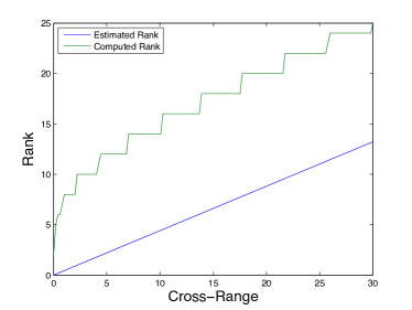
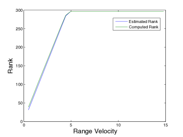
Figure 16: Comparison of the computed and estimated rank of $\mathcal{Y}$ for a single target. Left: Stationary target at various cross-range positions. Right: Moving target with various velocities.

We show in Figure 16 an illustration of this result. The left plot is for a stationary target and the right plot is for a moving target. The green line shows the numerically computed rank of the matrix $\mathcal{Y}$, while the blue line shows its asymptotic estimate (4.25). Note that both curves show the same growth. In the case of the stationary target there is a mismatch of the magnitude of the computed and estimated rank. This is because $n$ is not large enough in the simulation. A good approximation is obtained when $y_{j}\approx 0$ for $j\approx n$, because then we can approximate the series (4.22) that defines the symbol by the truncated sum for indices $|j|\leq n$. This is not the case in this simulation, so there is a discrepancy in the estimated rank. However, if we increase the aperture, thus increasing $n$, the result improves. Figure 17 illustrates this fact by showing how the rank normalized by the size of the matrix has the predicted asymptote as $n$ increases.

In the right plot of Figure 16 we compare the computed rank (in green) and the asymptotic estimate (4.25) (in blue) for a moving target located at $\vec{\boldsymbol{\rho}}=\vec{\boldsymbol{\rho}}_{o}$ at $s=0$. The rank is plotted as a function of the range component of the velocity. Note that, as expected, the rank increases with the velocity, and therefore with $|\alpha|$. For the moving target, the asymptotic estimate is in closer agreement to the computed one. This is because in this case the entries in the sequence $\{y_{j}\}_{j\in\mathbb{Z}}$ decay faster with $j$. Finally, we can observe that the rank is much larger for the moving target than the stationary target, even for small velocities.

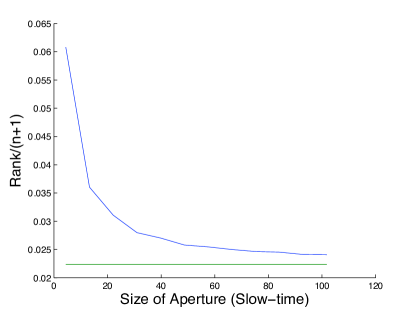
Figure 17: Convergence of the rank of $\mathcal{Y}$ normalized by the size $(n+1)$. The blue line is the computed value and the green line is the asymptotic estimate. The slow time sampling is fixed, so the longer the aperture is, the larger $n$.

4.4.2 Two targets

When there are two targets in the scene, we obtain from model (4.5) and the choice (4.6) of the pulse that

$$\mathcal{M}(s,t)=\sum_{j=1}^{2}\cos\left[\omega_{o}(t-\Delta\tau(s,\vec{\boldsymbol{\rho}}_{j}))\right]\exp\left[-\frac{B^{2}}{2}(t-\Delta\tau(s,\vec{\boldsymbol{\rho}}_{j}))^{2}\right].$$ (4.26)

We restrict the discussion to the case of two stationary targets. The extension to moving targets is straightforward. It amounts to adjusting the parameters $\alpha_{1}$ and $\alpha_{2}$ defined below in (4.28), by adding two linear terms in the target velocity, as in equation (4.20).

We obtain after a calculation given in detail in [2] that the entries of the matrix (4.17) are the discrete slow time samples of the function

$$\mathcal{Y}(s,s^{\prime}) \approx\frac{\sqrt{\pi}}{2B\Delta t}\left\{\sum_{j=1}^{2}\cos[\omega_{o}\alpha_{j}(s-s^{\prime})]\exp\left[-\frac{(B\alpha_{j})^{2}(s-s^{\prime})^{2}}{4}\right]\right.$$

$$+\cos[\omega_{o}(\alpha_{1}s-\alpha_{2}s^{\prime}+\beta)]\exp\left[-\frac{B^{2}(\alpha_{1}s-\alpha_{2}s^{\prime}+\beta)^{2}}{4}\right]$$ (4.27)

$$\left.+\cos[\omega_{o}(\alpha_{1}s^{\prime}-\alpha_{2}s+\beta)]\exp\left[-\frac{B^{2}(\alpha_{1}s^{\prime}-\alpha_{2}s+\beta)^{2}}{4}\right]\right\},$$

where

$$\alpha_{j}=-\frac{2V\vec{{\bf t}}\cdot\mathbb{P}_{o}(\vec{\boldsymbol{\rho}}_{j}-\vec{\boldsymbol{\rho}}_{o})}{cL},\quad j=1,2,$$ (4.28)

and

$$\beta=\frac{2}{c}\sum_{j=1}^{2}(-1)^{j}\left\{\vec{{\bf m}}_{o}\cdot(\vec{\boldsymbol{\rho}}_{j}-\vec{\boldsymbol{\rho}}_{o})+\frac{[\vec{{\bf m}}_{o}\cdot(\vec{\boldsymbol{\rho}}_{j}-\vec{\boldsymbol{\rho}}_{o})]^{2}}{2L}\right\}.$$ (4.29)

Thus, the matrix $\mathcal{Y}$ has a more complicated structure. The first term in (4.27), the sum over $j$, gives rise to a Toeplitz matrix, as before. The last two terms give matrices that are approximately g-Toeplitz or g-Hankel, depending on the sign of the ratio $\alpha_{2}/\alpha_{1}$.

Definition 1

An $(n+1)\times(n+1)$ g-Hankel matrix $\mathcal{H}$ with shift $g\in\mathbb{Z}^{+}$ is defined by a sequence $\{h_{j}\}_{j\in\mathbb{N}}$ as

$$\mathcal{H}_{j\ell}=h_{j-1+g(\ell-1)},\qquad j,\ell=1,\ldots,n+1.$$

The matrix is Hankel when $g=1$. A g-Toeplitz matrix is defined similarly, by replacing $g$ with $-g$.

It is easier to analyze the spectrum of the matrix $\mathcal{Y}$, when the reference point $\vec{\boldsymbol{\rho}}_{o}$ is chosen so that

$$\frac{\alpha_{2}}{\alpha_{1}}<0,\quad\mbox{and}\quad g:=\left|\frac{\alpha_{2}}{\alpha_{1}}\right|\in\mathbb{N}.$$ (4.30)

Then, $\mathcal{Y}$ is given by

$$\mathcal{Y}=\mathcal{T}+\mathcal{H}+\mathcal{H}^{T},$$ (4.31)

with the Toeplitz and g-Hankel matrices

$$\mathcal{T}_{j\ell}=y_{j-\ell},\qquad\mathcal{H}_{j\ell}=h_{(j-1)+g(\ell-1)},\qquad j,\ell=1,\ldots,n+1.$$ (4.32)

The sequences $\{y_{j}\}_{j\in\mathbb{Z}}$ and $\{h_{j}\}_{j\in\mathbb{N}}$ that define these matrices are

$$y_{j}=\frac{\sqrt{\pi}}{2B\Delta t}\sum_{\ell=1}^{2}\cos\left(\omega_{o}\Delta s|\alpha_{\ell}|j\right)e^{-\frac{(B\Delta s|\alpha_{\ell}|j)^{2}}{4}},$$ (4.33)

and

$$h_{j}=\frac{\sqrt{\pi}}{2B\Delta t}e^{-\frac{[B\Delta s|\alpha_{1}|(j+\zeta)]^{2}}{4}}\cos[\omega_{o}\Delta s|\alpha_{1}|(j+\zeta)],\qquad\zeta=\frac{\beta}{|\alpha_{1}|\Delta s}.$$ (4.34)

If the range offsets from the reference point $\vec{\boldsymbol{\rho}}_{o}$ are sufficiently large, so that

$$B|\beta|=\frac{2B}{c}\left|\sum_{\ell=1}^{2}(-1)^{\ell}\{\vec{{\bf m}}_{o}\cdot(\vec{\boldsymbol{\rho}}_{\ell}-\vec{\boldsymbol{\rho}}_{o})+\frac{[\vec{{\bf m}}_{o}\cdot(\vec{\boldsymbol{\rho}}_{\ell}-\vec{\boldsymbol{\rho}}_{o})]^{2}}{2L}\right|\gg 1,$$

then the g-Hankel matrix has small entries, and $\mathcal{Y}$ is approximately Toeplitz, as in the single target case. The meaning of this is that the difference of the travel times between the SAR platform and such targets is larger than the compressed pulse width, which makes their interaction in (4.27) negligible. However, if the range offsets are small, the interaction plays a role and the structure of the matrix $\mathcal{Y}$ is given by equation (4.31). In this case, the estimate of the rank of $\mathcal{Y}$ follows from the recent results in [21, 13, 14]. They state that the g-Hankel terms $\mathcal{H}+\mathcal{H}^{T}$ have a negligible effect on the rank in the limit $n\to\infty$. See [2] for more details. Thus, we can conclude in either case that the rank estimate of $\mathcal{Y}$ is given by equation (4.23), in terms of the symbol $\widehat{y}(\theta)$ defined by (4.22), using the sequence $\{y_{j}\}_{j\in\mathbb{Z}}$ with entries (4.33).

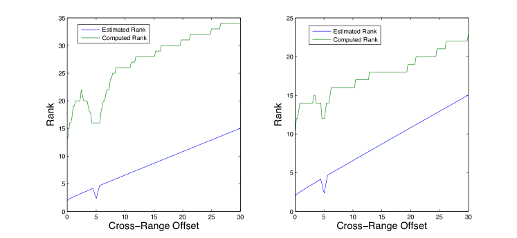
Figure 18: Computed and estimated rank of matrix $\mathcal{Y}$ for a scene with two stationary targets. On the left, one target is fixed at location $\vec{\boldsymbol{\rho}}_{1}=(5,5,0)$m and the location of the other varies on the line segment between $(-5,0.01,0)$m and $(-5,30,0)$m. On the right, one target is fixed at location $\vec{\boldsymbol{\rho}}_{1}=(0.15,5,0)$m and the location of the other varies on the line segment between $(-0.15,0.01,0)$m and $(-0.15,30,0)$m.

We plot in Figure 18 the computed and estimated rank for two different configurations of the stationary targets. The results on the left consider one target at location $\vec{\boldsymbol{\rho}}_{1}=(5,5,0)$m. The second target location is varied between $(-5,0.01,0)$m and $(-5,30,0)$m. The range separation is large, equal to $10$m, so the entries of the g-Hankel matrix $H$ are negligible because $B|\beta|=41.47\gg 1$. The plot on the right considers one target at $\vec{\boldsymbol{\rho}}_{1}=(0.15,5,0)$m and a second target at location the $\vec{\boldsymbol{\rho}}_{2}$ varying between $(-0.15,0.01,0)$m and $(-0.15,30,0)$ m. The range separation is now small, and the g-Hankel matrix $\mathcal{H}$ is no longer negligible. Nevertheless, as predicted by the asymptotic theory, the rank of matrix $\mathcal{Y}$ behaves essentially the same as before.

4.4.3 Conclusions of the analysis of rank

Several conclusions can be made from the analysis summarized above. First, the traces from a moving target form a high rank matrix. For a fixed number $n$ of slow time samples, the rank grows linearly with the target speed, until the matrix becomes full rank. The traces from a stationary target form a low rank matrix if the scene is small enough. The rank grows linearly with the cross-range offset of the target from the reference point $\vec{\boldsymbol{\rho}}_{o}$, but the growth is at a slower rate than for a moving target.

We also analyzed the rank for scenes with two stationary targets and found that it increases linearly with the cross-range offsets of the targets from $\vec{\boldsymbol{\rho}}_{o}$. The expectation, confirmed by the numerical simulations, is that the rank increases with the number of targets. This is why the data separation with robust PCA should be done in successive small time windows, with each window containing the traces from only a few stationary targets. These traces give a matrix that is low rank, and thus can be separated from the traces due to moving targets. The results shown in Figure 9 illustrate this point.

5 Numerical Simulations

We present here more numerical simulations that illustrate the performance of the annihilation filters defined in sections 3.1 and 3.4. We have presented already in sections 3.2 and 3.3 three different simulations for data separation with robust PCA. More results can be found in [2].

5.1 Setup of the simulations

We use the GOTCHA Volumetric SAR setup as described in section 4.1. The data traces are generated with the model (4.3). In all the simulations, the point targets are assumed to have identical reflectivity $\sigma_{q}=1$. The motion estimation results are obtained with the phase space algorithm introduced in [3]. This algorithm requires that we know the location of the target at one moment during the measurement window. We choose it at the center of the aperture, which is why there is no error in the target trajectory at $s=0$.

For the robust PCA results, the principal component pursuit optimization is solved with an augmented Lagrangian approach. It requires the computation of the top few singular values and corresponding singular vectors of large and sparse matrices, which we do with the software package PROPACK.

5.2 Annihilation Filters

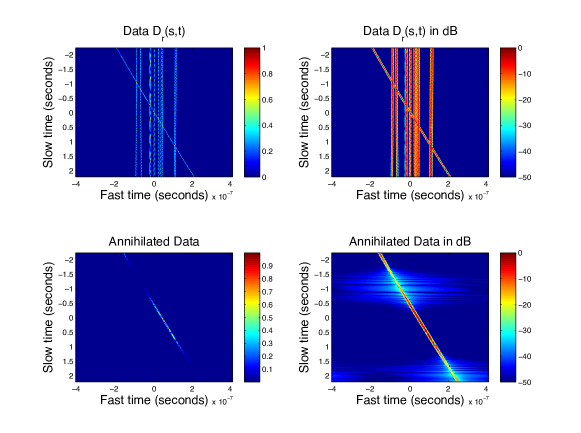
Figure 19: Data separation with the annihilation filter for a scene with ten stationary targets and a moving one. The top row shows the data traces and the bottom row the trace from the moving target, as separated by the algorithm. The right column is the left column plotted in dB scale.

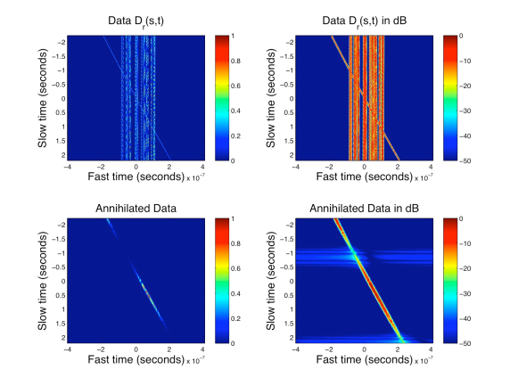
Figure 20: Data separation with the annihilation filter for a scene with thirty stationary targets and a moving one. The top row shows the data traces and the bottom row the trace from the moving target, as separated by the algorithm. The right column is the left column plotted in dB scale.

We give two examples of data separation with the annihilation filters described in section 3.1. In the first example, we have a complex scene composed of ten stationary scatterers in an imaging region of 50$\times$50$\mbox{m}^{2}$, and a moving target with velocity $\vec{\bf u}=28/\sqrt{2}(1,1,0)$m/s. We plot in the top row of Figure 19 the data traces, and in the bottom row the filtered traces. The right column is the same as the left except it is plotted in decibel (dB) scale to increase the contrast of the figure. The second example considers a scene with thirty stationary targets and the same one moving target. The results are in Figure 20. In both examples we used the exact stationary scatterer locations in the definition of the filters (3.4). The errors in the estimated target trajectories, with the separated trace from the moving target for each example, are shown in Figure 21.

Note that the filtering and the motion estimation results are worse in the second example, where there are more stationary targets to remove, by applying repeatedly filters like (3.4) to the traces. Computing many times numerical approximations of slow time derivatives causes errors to accumulate. This is specially because we have high frequency signals, and the sampling in slow time is limited by the pulse repetition frequency of the SAR system.

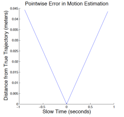
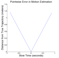
Figure 21: Error of the estimated target trajectory in a complex scene with ten stationary targets (left) and thirty stationary targets (right). The motion estimation is done with the filtered data shown in the bottom row of Figures 19 and 20.

5.3 Data separation for Scene 1

We already saw in section 3.3, Figure 11, the separation of the traces from the twenty stationary and two moving targets in Scene 1. Here we show the further separation of the traces from the moving targets, as described in section 3.4. The first moving target is located at $(0,0,0)$m at $s=0$, and is moving in the horizontal plane with velocity ${\bf u}=\frac{28}{\sqrt{2}}(1,1)$m/s. The second target is located at $(-5,5,0)$m at $s=0$, and moves with velocity ${\bf u}=\frac{14}{\sqrt{3}}\left(-1,\sqrt{2}\right)$m/s.

We apply the method described in section 3.3 to the traces shown in the right plot of Figure 11, separated by robust PCA. We estimate the velocity of the first target, apply the travel time transformation (3.17) to the traces, and then use the robust PCA approach to do the separation. The output of the data separation is shown in Figure 22. The traces from the stationary targets, as obtained by the robust PCA method are on the left. The traces from the two moving targets are in the middle and right plots. The images obtained with these traces are in Figure 23. All the targets, stationary and moving are now in focus. The peak of the image for the second moving target is slightly displaced in cross-range due to the error in its velocity estimation after separation.

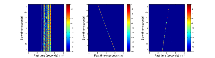
Figure 22: Data separation for Scene 1. Left: traces from the stationary targets. Middle and right: traces from the moving targets.

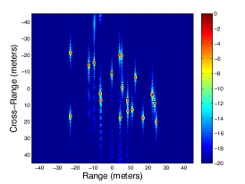
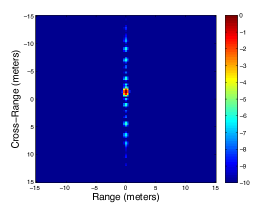
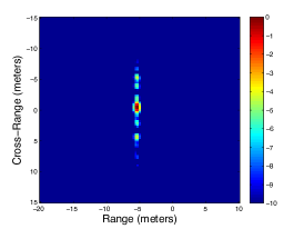
Figure 23: Images for Scene 1. Left: image with the traces from the stationary targets. Middle and right: image with the traces the moving targets.

6 Summary

We presented two approaches for separating the pulse and range compressed echoes from stationary and moving targets in a complex scene using a single synthetic aperture radar (SAR) antenna. The separation is required for estimating the motion of the targets and focusing the images.

The first approach subtracts the echoes from the stationary targets one by one, by performing the following four steps: (1) It estimates the stationary target location $\vec{\boldsymbol{\rho}}^{e}$ from a preliminary image. (2) It transforms the data using a map $\mathbb{T}_{+}^{\vec{\boldsymbol{\rho}}^{e}}$ so that the echo from the target becomes approximately independent of the SAR antenna location on the flight path. (3) It annihilates the target echo by exploiting this independence. (4) It undoes the transformation at step (2) by applying the map $\mathbb{T}_{-}^{\vec{\boldsymbol{\rho}}^{e}}$ to the remaining echoes.

The second approach is based on the robust principle component analysis (PCA) method, which is designed to decompose a matrix ${\cal M}$ into its low rank part and high rank but sparse part. In our context, the entries of the matrix ${\cal M}$ are the samples of the pulse and range compressed echoes measured by the SAR antenna. The main observation is that with appropriate pre-processing and windowing, the discrete samples of the stationary target echoes form a low rank matrix, while those from a few moving targets form a high rank sparse matrix. Thus, they can be separated with robust PCA.

We presented a brief analysis of the two methods, and a numerical comparison of their performance. Each method has its advantages and disadvantages, but they complement each other. Thus, we can combine them to improve the data separation results for complex and extended imaging scenes.

References

- [1] S. Barbarossa and A. Farina. Detection and imaging of moving objects with synthetic aperture radar. IEE Proceedings-F, 139(1):79–88, 1992.
- [2] L. Borcea, T. Callaghan, and G. Papanicolaou. Synthetic Aperture Radar Imaging and Motion Estimation via Robust Principal Component Analysis. arXiv:1208.3700, 2012.
- [3] L. Borcea, T. Callaghan, and G. Papanicolaou. Synthetic Aperture Radar Imaging with Motion Estimation and Autofocus. Inverse Problems, 28:045006, 2012.
- [4] L. Borcea, F. Gonzalez del Cueto, G. Papanicolaou, and C. Tsogka. Filtering deterministic layering effects in imaging. SIAM Multiscale Model. Simul., 7(3):1267–1301, 2009.
- [5] L. Borcea, F. Gonzalez del Cueto, G. Papanicolaou, and C. Tsogka. Filtering random layering effects in imaging. SIAM Multiscale Model. Simul., 8(3):751–781, 2010.
- [6] A. Böttcher and B. Silbermann. Introduction to Large Truncated Toeplitz Matrices. Springer, 1999.
- [7] E. J. Candès, X. Li, Y. Ma, and J. Wright. Robust Principal Component Analysis? Journal of ACM, 58(1):1–37, 2009.
- [8] M. Cheney. A mathematical tutorial on synthetic aperture radar. SIAM review, 43(2):301–312, 2001.
- [9] John C. Curlander and Robert N. McDonough. Synthetic Aperture Radar: Systems and Signal Processing. Wiley-Interscience, 1991.
- [10] Y. Ding and DC Munson Jr. Time-frequency methods in SAR imaging of moving targets. In IEEE International Conference on Acoustics, Speech, and Signal Processing, 2002. Proceedings.(ICASSP’02), volume 3, pages 2881–2884, 2002.
- [11] Y. Ding, N. Xue, and DC Munson Jr. An analysis of time-frequency methods in SAR imaging of moving targets. In Sensor Array and Multichannel Signal Processing Workshop. 2000. Proceedings of the 2000 IEEE, pages 221–225, 2000.
- [12] J. Ender. Detectability of slowly moving targets using a multi-channel SAR with an along-track antenna array. In Proceedings of SEE/IEE Conference (SAR 93), Paris, pages 19–22, 1993.
- [13] D. Fasino. Spectral properties of Toeplitz-plus-Hankel matrices. Calcolo, 33:87–98, 1996.
- [14] D. Fasino and P. Tilli. Spectral clustering properties of block multilevel Hankel matrices. Linear Algebra and its Applications, 306:155–163, 2000.
- [15] J. R. Fienup. Detecting Moving Targets in SAR Imagery by Focusing. IEEE Transactions on Aerospace and Electronic Systems, 37(3):794–809, 2001.
- [16] B. Friedlander and B. Porat. VSAR: a high resolution radar system for detection of moving targets. IEE Proc.-Radar, Sonar Navig., 144(4):205–218, 1997.
- [17] J. K. Jao. Theory of Synthetic Aperture Radar Imaging of a Moving Target. IEEE Transactions on Geoscience and Remote Sensing, 39(9):1984–1992, 2001.
- [18] Charles V. Jakowatz Jr., Daniel E. Wahl, Paul H. Eichel, Dennis C. Ghiglia, and Paul A. Thompson. Spotlight-mode synthetic aperture radar: A signal processing approach. Springer, New York, NY, 1996.
- [19] M. Kac, W. L. Murdock, and G. Szegő. On the eigenvalues of certain Hermitian forms. J. Rational Mech. Anal., (1):767–800, 1953.
- [20] M. Kirscht. Detection and imaging of arbitrarily moving targets with single-channel SAR. IEE Proc.-Radar Sonar Navig., 150(1):1984–1992, 2003.
- [21] E. Ngondiep, S Serra-Capizzano, and D. Sesana. Spectral Features and Asymptotic Properties for -Circulants and -Toeplitz Sequences. SIAM J. Matrix Anal. Appl., 31(4):1663–1687, 2010.
- [22] R. P. Perry, R. C. DiPietro, and R. L. Fante. SAR Imaging of Moving Targets. IEEE Transactions on Aerospace and Electronic Systems, 35(1):188–200, 1999.
- [23] T. Sparr. Time-Frequency Signatures of a Moving Target in SAR Images. Paper presented at the RTO SET Symposium on Target Identification and Recognition Using RF Systems, Oslo, Norway, 11-13 October, 2004. Published in RTO-MP-SET-080.
- [24] G. Wang, X. Xia, and V. Chen. Dual-Speed SAR Imaging of Moving Targets. IEEE Transactions on Aerospace and Electronic Systems, 42(1):368–379, 2006.
- [25] G. Wang, X. Xia, V. Chen, and R. Fiedler. Detection, Location, and Imaging of Fast Moving Targets Using Multifrequency Antenna Array SAR. IEEE Transactions on Aerospace and Electronic Systems, 40(1):345–355, 2004.
- [26] S. Zhu, G. Liao, Y. Qu, Z. Zhou, and X. Liu. Ground Moving Targets Imaging Algorithm for Synthetic Aperture Radar. IEEE Transactions on Geoscience and Remote Sensing, 49(1):462–477, 2011.