DAMTP-2012-68

Exact Kähler Potential from Gauge Theory and Mirror Symmetry

Jaume Gomis and Sungjay Lee

^aPerimeter Institute for Theoretical Physics,
Waterloo, Ontario, N2L 2Y5, Canada

^bDAMTP, Centre for Mathematical Sciences,
Cambridge University, Cambridge CB3 0WA, United Kingdom

1 Introduction

Two dimensional gauge theories – known as gauged linear sigma models (GLSM) – provide a variety of insights into the dynamics of nonlinear sigma models [1]. These two dimensional field theories – apart from mimicking ubiquitous phenomena in four dimensional gauge theories – play a central role in string theory. Specially, nonlinear sigma models on Calabi-Yau threefold target spaces, which give rise to a very rich set of vacua of string theory. The study of Calabi-Yau sigma models is at the genesis of several remarkable discoveries – including mirror symmetry [2, 3]– and has emerged as a source of inspiration for both physicists and mathematicians.

Physical observables in Calabi-Yau sigma models can receive non-perturbative corrections. These are generated by worldsheet instantons, which correspond to holomorphic maps from the worldsheet to the Calabi-Yau target space. Worldsheet instanton corrections to the point particle approximation correct the Kähler moduli space of the Calabi-Yau manifold into the so called “quantum Kähler moduli space”, from which effective Yukawa couplings among other observables can be computed. The problem of summing over all worldsheet instantons defines an interesting class of topological invariants, known as the Gromow-Witten invariants [4, 5]. One of the central themes in this research area is to develop methods to compute these invariants.

Recently – with Doroud and Le Floch – we have computed [6] the exact partition function of $\mathcal{N}=(2,2)$ gauge theories on $S^{2}$ (see also [7]). The partition function admits two alternative descriptions, either as an integral over the Coulomb branch or as sum over vortex and anti-vortex configurations on the Higgs vacua of the theory. Each representation yields complementary insights into the dynamics of these gauge theories. These results offer a new window into the exact dynamics of nonlinear sigma models on Kähler manifolds. Specifically on Calabi-Yau manifolds, since two dimensional $\mathcal{N}=(2,2)$ gauge theories which flow to an $\mathcal{N}=(2,2)$ superconformal field theory in the infrared provide an elegant framework to study Calabi-Yau sigma models [1] (see also [8]).

In [6] these exact results were applied to the study of worldsheet instantons in Calabi-Yau sigma models. The representation of the $S^{2}$ partition function as a sum over vortices at the north pole and anti-vortices at the south pole was used to explicitly confirm that the non-perturbative worldsheet instanton corrections to the Kähler moduli space de-singularize the quantum dynamics across the topology-changing flop transition [1, 9]. We further speculated that the exact partition function of $\mathcal{N}=(2,2)$ gauge theories on $S^{2}$ may provide a novel approach to the computation of worldsheet instantons in Calabi-Yau sigma models.

More recently, these speculations became a conjecture in an interesting paper by Jockers et al. [10]. These authors conjectured that the exact $S^{2}$ partition function $Z$ [6, 7] of an $\mathcal{N}=(2,2)$ gauge theory flowing to a sigma model on a Calabi-Yau computes the exact Kähler potential $\mathcal{K}$ on the quantum Kähler moduli space $\mathcal{M}$ of the Calabi-Yau

$$Z(\tau_{a},\bar{\tau}_{a})=e^{-\mathcal{K}(\tau_{a},\bar{\tau}_{a})}\,.$$ (1.1)

Here, $\tau_{a}$ are coordinates in $\mathcal{M}$ parametrizing the Kähler moduli of the Calabi-Yau, which correspond to the complexified Fayet-Iliopoulos parameters in the GLSM. Evidence for this conjecture was presented in [10] by extracting the Gromov-Witten invariants from the exact Kähler potential $\mathcal{K}$ via (1.1) and matching them with those computed in the literature using different methods. Remarkably, the partition function on $S^{2}$ [6, 7] was also used in [10] to predict new Gromov-Witten invariants, which pass all consistency checks.

In this paper we provide two alternative proofs of the conjecture (1.1). One derivation uses the gauge theory approach to Calabi-Yau sigma models provided by GLSM’s. We demonstrate that path integral on the squashed two-sphere in the limit in which the two-sphere is infinitely squashed describes a very specific overlap of ground states of the infrared conformal field theory, which is known from the work of Cecotti and Vafa [11] to compute the exact Kähler potential $\mathcal{K}$. By explicitly proving that the partition function on the squashed two-sphere does not depend on the squashing parameter, we arrive to (1.1). This chain of reasoning ends up relating the partition function on the round two-sphere with the exact Kähler potential in the quantum Kähler moduli space of the Calabi-Yau that emerges in the infrared.

We also compute the exact two-sphere partition function of $\mathcal{N}=(2,2)$ Landau-Ginzburg models with an arbitrary twisted superpotential $W$. The partition function takes the simple form

$$Z=\int dYd\overline{Y}e^{-4\pi irW(Y)-4\pi ir\overline{W}(\overline{Y})}\,,$$ (1.2)

where $r$ is the radius of the two-sphere. Landau-Ginzburg models capture the dynamics of Calabi-Yau non-linear sigma models in certain domains of the Kähler moduli space of a Calabi-Yau as well as serving as the mirror description of Calabi-Yau sigma models. We study the two-sphere partition function as a function of the space of marginal deformations of the underlying superconformal field theory – which span the Kähler moduli space $\mathcal{M}$ – and obtain a second derivation of the conjecture (1.1), now from the Landau-Ginzburg approach to Calabi-Yau sigma models.

We investigate mirror symmetry for sigma models on Kähler manifolds – including Calabi-Yau manifolds – from the viewpoint of the two-sphere partition function. This uses the results for the partition function of GLSM’s found in [6, 7] and the result (1.2) derived in this paper for Landau-Ginzburg models. We show that the $S^{2}$ partition function of the Landau-Ginzburg models put forward by Hori and Vafa [12] exactly reproduces the $S^{2}$ partition function for the mirror abelian GLSM’s, which describe toric varieties and complete intersections in toric varieties. For non-abelian GLSM’s we use the exact results on the two-sphere [6, 7] to rewrite the gauge theory partition function in Landau-Ginzburg form and prove a conjecture by Hori and Vafa [12] for the mirror Landau-Ginzburg description of these non-abelian GLSM’s.

The plan of the rest of the paper is as follows. In section 2 we construct the Lagrangian and supersymmetry transformations of $\mathcal{N}=(2,2)$ theories on the squashed two-sphere. In section 3 we provide a proof of the conjecture (1.1) in two steps. We first prove that the partition function on the squashed two-sphere is independent of the squashing parameter, while relegating many of the technical details of this proof to the Appendix. We then show that the path integral on the squashed two-sphere in the limit where the sphere is infinitely squashed provides a path integral representation of the ground state overlap which is known to compute the Kähler potential $\mathcal{K}$. In section 4 we construct the Lagrangian and supersymmetry transformations of $\mathcal{N}=(2,2)$ Landau-Ginzburg models with an arbitrary twisted superpotential $W$. We then use these results to give an alternative proof of the conjecture (1.1) as well as to establish the exact equivalence of the two-sphere partition function of GLSM’s and mirror Landau-Ginzburg models.

2 Supersymmetric Theories on Squashed Two-Sphere

The partition function of $\mathcal{N}=(2,2)$ gauge theories on $S^{2}$ was computed in [6, 7]. These theories are invariant under the $SU(2|1)$ algebra, which is the $\mathcal{N}=(2,2)$ supersymmetry algebra on $S^{2}$. In order for a field theory to be supersymmetric on $S^{2}$, the theory must admit a $U(1)$ $R$-symmetry, as the associated conserved charge $R$ appears in the anticommutator of supercharges in $SU(2|1)$.

In this section we construct the supersymmetry transformations and supersymmetric action for $\mathcal{N}=(2,2)$ gauge theories on the squashed two-sphere $S^{2}_{b}$. As we shall see, the existence of a $U(1)$ $R$-symmetry plays an important role in the construction of these theories.

As we shall see, the study of the partition function of $\mathcal{N}=(2,2)$ gauge theories on the squashed two-sphere provides a path towards proving the conjecture (1.1). In section 4.2 an alternative approach to the derivation of (1.1) is presented.

2.1 Superalgebra and Killing Spinors on Squashed Two-Sphere

Let us consider deforming the round sphere to the squashed two-sphere $S^{2}_{b}$ while preserving a $U(1)\subset SU(2)$ isometry. The squashed two-sphere can be described by an embedding equation in $\mathbb{R}^{3}$

$$\frac{x_{1}^{2}+x_{2}^{2}}{l^{2}}+\frac{x_{3}^{2}}{\tilde{l}^{2}}=1\ ,$$ (2.1)

which depends on the dimensionless squashing parameter $b=l/\tilde{l}$. The metric on the squashed two-sphere is

$$ds^{2}=f^{2}(\theta)d\theta^{2}+l^{2}\sin^{2}\theta d\varphi^{2}\,,$$ (2.2)

where $f^{2}(\theta)=\tilde{l}^{2}\sin^{2}\theta+l^{2}\cos^{2}\theta$. The vielbein in a patch around the equator excluding the north and south poles of $S^{2}_{b}$ is chosen as

$$e^{\hat{1}}=f(\theta)d\theta\ ,\qquad e^{\hat{2}}=l\sin\theta d\varphi\,.$$ (2.3)

In this patch, the spin connection on $S^{2}_{b}$ is given by

$$\omega\equiv\omega_{\hat{1}\hat{2}}=-\frac{l\cos\theta}{f(\theta)}d\varphi\,.$$ (2.4)

Later we consider vielbein and spin connection which are smooth in a patch near the north and the south poles of $S^{2}_{b}$ to analyze the physics near the poles.

Since squashing the $S^{2}$ breaks the $SU(2)$ symmetry down to $U(1)$, the supercharges on $S^{2}$ that do not generate the $U(1)$ symmetry of $S^{2}_{b}$ must be broken on the squashed two-sphere. This implies that the supersymmetry algebra on the squashed two-sphere is an $SU(1|1)$ subalgebra of $SU(2|1)$

$$\mathcal{Q}^{2}=J+\frac{R}{2}\ ,\qquad\Big{[}J+\frac{R}{2},\mathcal{Q}\Big{]}=0\,,$$ (2.5)

where $J$ corresponds to the $U(1)$ subgroup of the $SU(2)$ symmetry preserving $S^{2}_{b}$ and $R$ is the $U(1)$ $R$-symmetry generator in $SU(2|1)$. We note that this is precisely the supersymmetry algebra generated by the supercharge used in [6]

$$\mathcal{Q}=S_{1}+Q_{2}\,$$ (2.6)

to localize the path integral of $\mathcal{N}=(2,2)$ gauge theories on $S^{2}$.

While bosonic space-time transformations are parametrized by Killing vectors, Killing spinors parametrize supersymmetry transformations. On the round two-sphere $S^{2}$ of radius $l$, the supersymmetry parameters $\epsilon$ and $\bar{\epsilon}$ corresponding to the supercharge $\mathcal{Q}$ in (2.6) are conformal Killing spinors, which can be taken to satisfy

$$\nabla_{i}\epsilon=+\frac{1}{2l}\gamma_{i}\gamma^{3}\epsilon\,,\qquad\nabla_{i}\bar{\epsilon}=-\frac{1}{2l}\gamma_{i}\gamma^{3}\bar{\epsilon}\,.$$ (2.7)

In the patch near the equator defined by the vielbein (2.3), they are explicitly given by [6]

$$\epsilon=e^{-\frac{i}{2}\gamma^{\hat{2}}\theta}e^{+\frac{i}{2}\varphi}\epsilon_{\circ}\ ,\ \text{ with }\ \gamma^{3}\epsilon_{\circ}=+\epsilon_{\circ}\ ,$$

$$\bar{\epsilon}=e^{+\frac{i}{2}\gamma^{\hat{2}}\theta}e^{-\frac{i}{2}\varphi}\bar{\epsilon}_{\circ}\ ,\ \text{ with }\ \gamma^{3}\bar{\epsilon}_{\circ}=-\bar{\epsilon}_{\circ}\ .$$ (2.8)

Killing spinors generating the $SU(1|1)$ supersymmetry transformations on the squashed two-sphere $S^{2}_{b}$ can be found by turning on a background gauge field $V_{i}$ for the $U(1)$ $R$-symmetry, just as on the squashed three-sphere [13]. The Killing spinors on $S^{2}_{b}$ satisfy a generalized Killing spinor equation

$$D_{i}\epsilon=\frac{1}{2f(\theta)}\gamma_{i}\gamma^{3}\epsilon\,,\qquad\qquad D_{i}\bar{\epsilon}=-\frac{1}{2f(\theta)}\gamma_{i}\gamma^{3}\bar{\epsilon}\,,$$ (2.9)

where the covariant derivative $D_{i}$ includes the background gauge connection for the $U(1)$ $R$-symmetry

$$D_{i}\epsilon=\left(\nabla_{i}-iV_{i}\right)\epsilon\ ,\qquad D_{i}\bar{\epsilon}=\left(\nabla_{i}+iV_{i}\right)\bar{\epsilon}\,,$$ (2.10)

and we have taken into account that the $R$-charge of $\epsilon$ is $1$ and that of $\bar{\epsilon}$ is $-1$. With the choice of connection

$$V=\frac{1}{2}\left(1-\frac{l}{f(\theta)}\right)d\varphi\,,$$ (2.11)

the Killing spinors on $S^{2}_{b}$ in the patch near the equator of the squashed two-sphere are given by (2.8). These generate the $SU(1|1)$ transformations on the squashed two-sphere. We collect useful identities obeyed by the Killing spinors on the squashed two-sphere which are frequently used throughout the paper in the Appendix.

We note that the background connection for the $U(1)$ $R$-symmetry (2.11) is topologically trivial and is defined everywhere on the squashed two-sphere, unlike the vielbein and spin connection, that need to be defined in coordinate patches.

2.2 Supersymmetric Lagrangian on Squashed Two-Sphere

The supersymmetry transformations are similar to those on the round two-sphere $S^{2}$ once the background gauge field $V_{i}$ is coupled to the various fields according to their $U(1)$ $R$-charges and we take into account the generalized Killing spinor equation (2.9). As explained in [6], the supersymmetry transformations are completely determined by demanding that the supersymmetry transformations of the theory in flat space are covariant under Weyl transformations (see Appendix B of [6] for more details).

Let us begin with the supersymmetry transformations and Lagrangian for the vector multiplet. The transformation laws generated by the supercharge $\mathcal{Q}$ are given by

$$\delta\lambda= (iV_{m}\gamma^{m}-{\rm D})\epsilon$$

$$\delta\bar{\lambda}= (i\bar{V}_{m}\gamma^{m}+{\rm D})\bar{\epsilon}$$

$$\delta A_{i}= -\frac{i}{2}\Big{(}\bar{\epsilon}\gamma_{i}\lambda-\bar{\lambda}\gamma_{i}\epsilon\Big{)}$$

$$\delta\sigma_{1}= \frac{1}{2}\Big{(}\bar{\epsilon}\lambda-\bar{\lambda}\epsilon\Big{)}$$

$$\delta\sigma_{2}= -\frac{i}{2}\Big{(}\bar{\epsilon}\gamma_{3}\lambda-\bar{\lambda}\gamma_{3}\epsilon\Big{)}$$

$$\delta D= -\frac{i}{2}\bar{\epsilon}\not{D}\lambda-\frac{i}{2}\big{[}\sigma_{1},\bar{\epsilon}\lambda\big{]}-\frac{1}{2}\big{[}\sigma_{2},\bar{\epsilon}\gamma^{3}\lambda\big{]}+\frac{i}{2}\epsilon\not{D}\bar{\lambda}-\frac{i}{2}\big{[}\sigma_{1},\bar{\lambda}\epsilon\big{]}-\frac{1}{2}\big{[}\sigma_{2},\bar{\lambda}\gamma^{3}\epsilon\big{]}\,,$$ (2.12)

with $\epsilon$ and $\bar{\epsilon}$ the Killing spinors on $S^{2}_{b}$ and $V_{m}$ and ${\bar{V}}_{m}$ defined by

$$V_{m}= \Big{(}+D_{1}\sigma_{1}+D_{2}\sigma_{2},\ +D_{2}\sigma_{1}-D_{1}\sigma_{2},\ F_{\hat{1}\hat{2}}+i[\sigma_{1},\sigma_{2}]+\frac{1}{f(\theta)}\sigma_{1}\Big{)}\ ,$$

$$\bar{V}_{m}= \Big{(}-D_{1}\sigma_{1}+D_{2}\sigma_{2},\ -D_{2}\sigma_{1}-D_{1}\sigma_{2},\ F_{\hat{1}\hat{2}}-i[\sigma_{1},\sigma_{2}]+\frac{1}{f(\theta)}\sigma_{1}\Big{)}\ .$$ (2.13)

Note that in all formulas the covariant derivative $D_{i}$ includes the gauge, local Lorentz and $U(1)$ $R$-symmetry connections. These supersymmetry transformations close off-shell and realize $SU(1|1)$ on the vector multiplet fields.

The Lagrangian for a vector multiplet takes the following form

$${\cal L}_{\text{v.m.}} =\frac{1}{2g^{2}}\text{Tr}\bigg{[}\left(F_{\hat{1}\hat{2}}+\frac{\sigma_{1}}{f(\theta)}\right)^{2}+(D_{i}\sigma_{1})^{2}+(D_{i}\sigma_{2})^{2}-[\sigma_{1},\sigma_{2}]^{2}+{\rm D}^{2}$$

$$\qquad\qquad\ \ +i\bar{\lambda}\gamma^{i}D_{i}\lambda+i\bar{\lambda}[\sigma_{1},\lambda]+\bar{\lambda}\gamma^{3}[\sigma_{2},\lambda]\bigg{]}\ ,$$ (2.14)

which can be shown to be invariant under the supersymmetry transformations (2.12). For each $U(1)$ factor in the gauge group $G$, a supersymmetric Fayet-Iliopoulos (FI) ${\rm D}$-term can be added

$${\cal L}_{\text{FI}}=-i\xi\text{Tr}\left[{\rm D}-\frac{\sigma_{2}}{f(\theta)}\right]\ ,$$ (2.15)

as well as a two-dimensional theta angle

$${\cal L}_{\text{top}}=-i\frac{\vartheta}{2\pi}\text{Tr}F\ .$$ (2.16)

We now in turn consider a chiral multiplet charged in some representation of the gauge group $G$. The supersymmetry transformations for a chiral multiplet of $R$-charge $-q$ are given by

$$\delta\phi= \bar{\epsilon}\psi\$$

$$\delta\bar{\phi}= \epsilon\bar{\psi}\ ,$$

$$\delta\psi= +i\gamma^{i}\epsilon D_{i}\phi+i\epsilon\sigma_{1}\phi+\gamma^{3}\epsilon\sigma_{2}\phi+i\frac{q}{2f(\theta)}\gamma_{3}\epsilon\phi+\bar{\epsilon}F\$$

$$\delta\bar{\psi}= -i\bar{\epsilon}\gamma^{i}D_{i}\bar{\phi}+i\bar{\epsilon}\bar{\phi}\sigma_{1}+\bar{\epsilon}\gamma^{3}\bar{\phi}\sigma_{2}+i\frac{q}{2f(\theta)}\bar{\epsilon}\gamma_{3}\bar{\phi}+\epsilon\bar{F}\$$

$$\delta F= \epsilon\Big{(}i\gamma^{i}D_{i}\psi-i\sigma_{1}\psi+\gamma^{3}\sigma_{2}\psi-i\lambda\phi\Big{)}-i\frac{q}{2}\psi\gamma^{i}D_{i}\epsilon\$$

$$\delta\bar{F}= \bar{\epsilon}\Big{(}i\gamma^{i}D_{i}\bar{\psi}-i\bar{\psi}\sigma_{1}-\gamma^{3}\bar{\psi}\sigma_{2}+i\bar{\phi}\lambda\Big{)}-i\frac{q}{2}\bar{\psi}\gamma^{i}D_{i}\bar{\epsilon}\,.$$ (2.17)

One can explicitly show that the supersymmetry algebra also closes off-shell for the chiral multiplet.

The $SU(1|1)$ invariant Lagrangian for a chiral multiplet of $R$-charge $-q$ is

$${\cal L}_{\text{c.m.}} =D_{i}\bar{\phi}D^{i}\phi+\bar{\phi}\left[\sigma_{1}^{2}+\sigma_{2}^{2}+i\frac{q-1}{f(\theta)}\sigma_{2}-\frac{q^{2}}{4f(\theta)^{2}}+\frac{q}{4}{\cal R}\right]\phi+\bar{F}F+i\bar{\phi}{\rm D}\phi$$

$$\ \ \ -i\bar{\psi}\gamma^{i}D_{i}\psi+\bar{\psi}\left[i\sigma_{1}-\left(\sigma_{2}+i\frac{q}{2f(\theta)}\right)\gamma^{3}\right]\psi+i\bar{\psi}\lambda\phi-i\bar{\phi}\bar{\lambda}\psi\ ,$$ (2.18)

where ${\cal R}$ denotes the curvature scalar of the squashed two-sphere. A supersymmetric superpotential ${\cal W}$ term for chiral multiplets

$${\cal L}_{\cal W}=F_{\cal W}+{\bar{F}}_{\cal W}\ ,$$ (2.19)

can be added provided that the superpotential carries $R$-charge $-2$, i.e., $q_{\cal W}=2$. The supersymmetric superpotential couplings (2.19) are precisely those of the theory in flat space, even though the action of a supersymmetric theory on curved space is generically corrected by $1/r$ terms [14].

When the theory has a flavour symmetry group $G_{F}$, we can turn on a supersymmetric background expectation value for a non-dynamical $G_{F}$ vector multiplet. This introduces twisted masses $m$ for the chiral multiplets. As we shall prove, the twisted masses $m$ and $R$-charges $q$ appear in the expression we derive for the partition function in the holomorphic combination

$$M=m+i{q\over 2l}\,.$$ (2.20)

These take values in the Cartan subalgebra of $G_{F}$.

It is also possible to introduce twisted chiral multiplets preserving supersymmetry on the squashed-sphere. Even though twisted chiral multiplets must be neutral under conventional vector multiplets, these multiplets play an important role in mirror symmetry and we will consider them in detail in section 4. As we shall see, the supersymmetrized twisted superpotential $W$ couplings on the squashed two-sphere are modified in comparison to the theory in flat space. These modifications have interesting physical implications.

3 A Proof of the Conjecture

The main conjecture that we want to prove states that whenever a Calabi-Yau manifold admits a Gauged Linear Sigma Model (GLSM) description, then the exact partition function of the GLSM on the round two-sphere [6, 7] determines the exact Kähler potential in the quantum Kähler moduli space, including all worldsheet instanton corrections. The explicit conjecture is

$$Z\left(\tau_{a},{\bar{\tau}}_{a}\right)=e^{-\mathcal{K}\left(\tau_{a},\bar{\tau}_{a}\right)}\,.$$ (3.1)

This conjecture [10] successfully passes several nontrivial tests and has been used to predict new Gromov-Witten invariants for a Calabi-Yau manifold for which no mirror Calabi-Yau is known.

Before delving into a proof of this conjecture, we will make a few preparatory remarks. In the GLSM approach to nonlinear sigma models on Calabi-Yau manifolds, the moduli of the Calabi-Yau map to parameters in the associated GLSM. The complex structure deformations of the Calabi-Yau manifold appear as parameters in the superpotential $\mathcal{W}$. These parameters can be interpreted as background expectation values for chiral multiplets. The (complexified) Kähler parameters of the Calabi-Yau appear instead in the twisted superpotential $W$ (see section 4.1 for more details) and correspond in the GLSM to the complexified FI parameters

$$\tau_{a}={\vartheta_{a}\over 2\pi}+i\xi_{a}\,.$$ (3.2)

These can be interpreted as background expectation values for twisted chiral multiplets.

Since the superpotential couplings (2.19) on the (squashed) two-sphere are the same as in flat space and ${\cal Q}$-exact, standard decoupling arguments [1] show that the GLSM partition function on the (squashed) two-sphere does not depend on the superpotential. The only constraint on the superpotential is that it carries $R$-charge $-2$, so that it can be coupled supersymmetrically to the (squashed) two-sphere. The partition function of the GLSM on the (squashed) two-sphere is, however, a non-trivial function of the complexified FI parameters, which are coordinates on the quantum Kähler moduli space of the Calabi-Yau.

Compact, non-singular Calabi-Yau manifolds do not admit continous isometries. This is realized in the associated superpotential $\mathcal{W}$ of the GLSM breaking all the symmetries of the GLSM kinetic terms. The absence of flavour symmetries forbids the addition of twisted masses $m$ for the chiral multipliets. Since the $R$-charges $-q$ of the fields are fixed by demanding that the superpotential $\mathcal{W}$ has $R$-charge $-q_{\cal W}=-2$ and no flavor symmetries, we conclude that the partition function on the (squashed) two-sphere for compact Calabi-Yau GLSM’s are non-trivial functions of the complexified Kähler moduli, as summarized in the notation $Z(\tau_{a},\bar{\tau}_{a})$. This is precisely the data that enters in the exact Kähler potential in the quantum Kähler moduli space of a compact Calabi-Yau. This provides a simple consistency check on the conjecture.

As already mentioned in [10], the Kähler potential $\mathcal{K}$ is known from the work of Cecotti and Vafa [11] to compute the inner product between certain ground states in the $\mathcal{N}=(2,2)$ superconformal field theory to which the GLSM flows in the infrared. This inner product is a function of the Calabi-Yau Kähler moduli. These moduli, in turn, correspond to marginal operators in the $\mathcal{N}=(2,2)$ superconformal field theory. These operators are superconformal descendants of operators in the twisted chiral ring of the conformal field theory. The Kähler potential in the quantum Kähler moduli space is given by [11]

$$\mathcal{K}(\tau_{a},\bar{\tau}_{a})=-\text{log}\ {}_{\text{R}}\langle\bar{0}|0\rangle_{\text{R}}\ ,$$ (3.3)

where $|0\rangle_{\text{R}}$ denotes the canonical supersymmetric vacuum in the Ramond sector while ${}_{\text{R}}\langle\bar{0}|$ denotes the conjugate to the canonical vacuum. We return to this below and refer to reference [11] for more details regarding the relation between the Kähler potential and this overlap of states.

We present in the rest of this section a physical proof of the above conjecture, completed in the following two steps. We first compute the exact partition function on the squashed two-sphere $S_{b}^{2}$, denoted by $Z_{b}$, and prove that $Z_{b}$ is independent of the squashing parameter $b$. In particular, it equals the partition function $Z$ on the round two-sphere. In section 4.2 we find an alternative proof of the conjecture using Landau-Ginzburg models.

We then show that the path integral on the squashed two-sphere $S^{2}_{b}$ in the degenerate limit $b\to 0$ yields a path integral representation of the overlap ${}_{\text{R}}\big{\langle}\bar{0}|0\big{\rangle}_{\text{R}}$ of the canonical ground states in the Ramond sector of the ${\cal N}=(2,2)$ superconformal field theory. Combining these two results, we arrive at the very relation we were aiming to prove

$$Z(\tau_{a},\bar{\tau}_{a})=Z_{b}(\tau_{a},\bar{\tau}_{a})\overset{b\to 0}{=}\ _{R}\big{\langle}\bar{0}|0\big{\rangle}_{\text{R}}\,=e^{-\mathcal{K}(\tau_{a},\bar{\tau}_{a})}\ .$$ (3.4)

It is well known, however, that the Kähler potential $\mathcal{K}$ is only defined up to Kähler transformations. These act as follows

$$\mathcal{K}(\tau,\bar{\tau})\rightarrow\mathcal{K}(\tau,\bar{\tau})+f(\tau)+\bar{f}(\bar{\tau})\,.$$ (3.5)

This raises a question: what is the gauge theory counterpart of this ambiguity? This ambiguity is mirrored in the choice of supersymmetric couplings on the (squashed) two-sphere for the background twisted chiral multiplet fields corresponding to the complexified FI parameters $\tau_{a}$. As shown in section 4.1, the inclusion of a twisted superpotential $W$ for the background twisted chiral multiplet changes the partition on the (squashed) two-sphere to

$$Z(\tau_{a},\bar{\tau}_{a})\rightarrow Z(\tau_{a},\bar{\tau}_{a})\exp\left(-4\pi ilW(\tau_{a})-4\pi il\overline{W}(\bar{\tau}_{a})\right)\,.$$ (3.6)

Therefore, both the Kähler potential $\mathcal{K}$ and the GLSM partition function $Z$ are only defined up to Kähler transformations.

The next two subsections are devoted to proving the two main claims summarized above.

3.1 Exact Partition Function

We compute in this section the partition function $Z_{b}$ of $\mathcal{N}=(2,2)$ gauge theories on the squashed two-sphere $S^{2}_{b}$ by supersymmetric localization. We perform the computation for an arbitrary gauge theory, including GLSM’s for arbitrary Kähler manifolds. After a technical computation, we prove that the partition function $Z_{b}$ is independent of the squashing parameter. This result is key in establishing the equivalence of the partition function of $\mathcal{N}=(2,2)$ gauge theories on the round $S^{2}$ with the exact Kähler potential in the quantum corrected Kähler moduli space of Calabi-Yau manifolds. To keep the flow of ideas clear, we relegate many of the technical details of the computation to the Appendix.

In a localization computation, the path integral restricts to the space of supersymmetric field configurations annihilated by a choice of supercharge. As mentioned earlier, the supercharge ${\cal Q}$ that generates the $SU(1|1)$ supersymmetry algebra is precisely the same one that was used in [6, 7] to localize the partition function $Z$ of $\mathcal{N}=(2,2)$ gauge theories on the round two-sphere $S^{2}$. Depending on the choice of deformation term (or contour), as shown in [6, 7], the partition function on $S^{2}$ can be localized to supersymmetric configurations either in the Coulomb branch or in the Higgs branch. The Coulomb branch configurations appear in the Coulomb phase of the gauge theory, while the Higgs branch configurations, which correspond to vortices at the north pole and anti-vortices at the south pole, appear in the Higgs phase of the theory. This yields two alternative but equal representations of the partition function $Z$: the Coulomb and Higgs branch representation.

In order to prove that the partition function $Z_{b}$ on $S^{2}_{b}$ is independent of the squashing parameter $b$ it suffices to localize the partition function on the squashed two-sphere to the Coulomb branch. Generalizing the analysis of saddle points of [6, 7] to the squashed two-sphere, we find that the path integral localizes onto the moduli space of solutions of the set of equations

$$D_{\hat{i}}\sigma_{1}=D_{\hat{i}}\sigma_{2}=0\ ,\qquad\left[\sigma_{1},\sigma_{2}\right]=0\,,\qquad F_{\hat{1}\hat{2}}+\frac{\sigma_{1}}{f(\theta)}=0\,.$$ (3.7)

Nontrivial gauge field configurations can be characterized by their flux through the squashed two-sphere

$$\frac{1}{2\pi}\int_{S^{2}_{b}}F=B\,,$$ (3.8)

where $B$ takes values in the Cartan subalgebra $\mathfrak{t}$ of $G$ and is GNO-quantized. The most general smooth solution to the saddle point equations (3.7) is

$$A=\frac{B}{2}\left(\kappa-\cos\theta\right)d\varphi\ ,\qquad\sigma_{1}=-\frac{B}{2l}\ ,\qquad\sigma_{2}=\sigma\ ,$$ (3.9)

where $\sigma$ is valued in the Lie algebra of $G$ and subject to the constraint

$$[\sigma,B]=0\,.$$ (3.10)

It is noteworthy that the vector multiplet Lagrangian (2.14) and the chiral multiplet Lagrangian (2.18) are both $\mathcal{Q}$-exact. More precisely

$${\cal L}_{\text{v.m.}} =-\frac{1}{g^{2}}\delta_{\mathcal{Q}}\delta_{\bar{\epsilon}}\ \text{Tr}\left(\frac{1}{2}\bar{\lambda}\gamma^{3}\lambda-2i{\rm D}\sigma_{2}+{i\over f(\theta)}\sigma_{2}^{2}\right)\ ,$$

$${\cal L}_{\text{c.m.}} =-\delta_{\mathcal{Q}}\delta_{\bar{\epsilon}}\left(\bar{\psi}\gamma^{3}\psi-2\bar{\phi}\sigma_{2}\phi-i\frac{q-1}{f(\theta)}\bar{\phi}\phi\right)\ .$$ (3.11)

This implies that the partition function of $\mathcal{N}=(2,2)$ gauge theories on the squashed two-sphere $S^{2}_{b}$ is independent of the super-renormalizable gauge couplings $g$. Furthermore, the superpotential couplings (2.19), which must have $R$-charge $-2$ to be supersymmetric on $S^{2}_{b}$, are also $\mathcal{Q}$-exact. Therefore the partition function $Z_{b}$ does not depend on the complex parameters that enter in the superpotential. It does depend, however, on the complexified FI parameters $\tau_{a}$, and the $R$-charges $-q$ and twisted masses $m$ associated to the flavour symmetry group $G_{F}$ of the gauge theory, which capture the isometries of the associated Kähler manifold.

We can compute the partition function by evaluating the Gaussian integral around the saddle point field configurations (3.9) using as the $\mathcal{Q}$-exact deformation term the vector and chiral multiplet Lagrangians ${\cal L}_{\text{v.m.}}$ and ${\cal L}_{\text{c.m.}}$, as well as a $\mathcal{Q}$-exact regulator term (A.6) given in the Appendix. The one-loop determinant for the vector multiplet fields once we take into account the Jacobian factor reducing the integral over $\sigma$ with the constraint $[\sigma,B]=0$ to an integral over the Cartan subalgebra is

$$Z^{\text{v.m.}}_{\text{one-loop}}(\sigma,B)\cdot J(\sigma,B)=\frac{1}{|\mathcal{W}(H_{B})|}\prod_{\begin{subarray}{c}\alpha\in\Delta^{+}\end{subarray}}\left[\left(\frac{\alpha\cdot B}{2l}\right)^{2}+\left(\alpha\cdot\sigma\right)^{2}\right]\,.$$ (3.12)

$\alpha$ are the roots of the Lie algebra of $G$ and $\mathcal{W}(H_{B})$ is the Weyl group of the symmetry group $H_{B}\subset G$ left unbroken by the flux. The one-loop determinant for a chiral multiplet transforming in a representation $\bf R$ of $G$ is

$$Z_{\text{one-loop}}^{\text{c.m.}}(\sigma,B,m,q) =\prod_{w\in\bf R}(-i)^{w\cdot B}(-1)^{|w\cdot B|/2}\frac{\Gamma\left({q\over 2}-il({w}\cdot\sigma+m)+{|{w}\cdot B|\over 2}\right)}{\Gamma\left(1-{q\over 2}+il({w}\cdot\sigma+m)+{|{w}\cdot B|\over 2}\right)}\,,$$ (3.13)

where $w$ are the weights of the representation $\bf R$ of $G$.

Combining the one-loop determinants with the classical contribution and summing over magnetic fluxes $B$ and integrating over the moduli space parametrized by $\sigma$, we get that the $S^{2}_{b}$ partition function of an $\mathcal{N}=(2,2)$ gauge theory is given by

$$Z_{b}(\tau_{a},\bar{\tau}_{a},M)= \sum_{B}\frac{1}{|\mathcal{W}(H_{B})|}\int_{\mathfrak{t}}d\sigma\,e^{-4\pi i\xi_{\rm ren}l\text{Tr}\sigma+i\vartheta\text{Tr}B}\prod_{\alpha\in\Delta^{+}}\left[\left(\frac{\alpha\cdot B}{2l}\right)^{2}+\left(\alpha\cdot\sigma\right)^{2}\right]$$ (3.14)

$$\hskip 8.5359pt\prod_{w\in\bf R}(-i)^{w\cdot B}(-1)^{|w\cdot B|/2}\frac{\Gamma\left({q\over 2}-il({w}\cdot\sigma+m)+{|{w}\cdot B|\over 2}\right)}{\Gamma\left(1-{q\over 2}+il({w}\cdot\sigma+m)+{|{w}\cdot B|\over 2}\right)}\ .$$

The partition function depends on the complexified FI parameters $\tau$ and on the mass $m$ and $R$-charges $-q$ of the chiral multiples through the holomorphic combination $M$ (2.20).

The conclusion of this computation is that the partition function on the squashed two-sphere $S^{2}_{b}$ is independent of the squashing parameter $b$. This is the first result needed in our proof of the main conjecture (1.1). In particular, the partition function of the round two-sphere $Z:=Z_{b=1}$ is identical to that of the squashed two-sphere

$$Z(\tau_{a},\bar{\tau}_{a},M)=Z_{b}(\tau_{a},\bar{\tau}_{a},M)\,.$$ (3.15)

Next, we use the freedom to change the squashing parameter $b$ to show that the partition function on the squashed two-sphere $S^{2}_{b}$ in the limit $b\rightarrow 0$ provides a path integral representation of the sought after overlap of states ${}_{\text{R}}\langle\bar{0}|0\rangle_{\text{R}}$.

3.2 Degenerate Limit and Ground State Inner Product

We now show that the partition function on the squashed two-sphere $S^{2}_{b}$ in the degenerate limit $b\to 0$ provides the path integral representation of ${}_{\text{R}}\langle\bar{0}|0\rangle_{\text{R}}$ :

$$Z_{b}(\tau_{a},\bar{\tau}_{a})\overset{b\to 0}{=}\ _{\text{R}}\langle\bar{0}|0\rangle_{\text{R}}\ .$$ (3.16)

Here we focus on GLSM’s that flow in the infrared to $\mathcal{N}=(2,2)$ superconformal field theories, which describe nonlinear sigma models on Calabi-Yau manifolds.

Let us first consider the path integral of a two dimensional ${\cal N}=(2,2)$ theory on a hemisphere. This path integral produces the wavefunction for a state which is prepared at the boundary of the hemisphere. This state is in the same cohomology class as the ground state. The projection to the actual ground state can be obtained through the following canonical construction [11]. We attach to the hemisphere a long “neck” to project into the actual ground state. More precisely, let us imagine that a semi-infinite cylinder is attached to the boundary of the hemisphere. Introducing such a semi-infinite cylinder evolves the state $|\Psi\rangle$ on the boundary of the hemisphere into a state $e^{-HT}|\Psi\rangle$ where $T\to\infty$. This evolution can be understood as a projection of the state $|\Psi\rangle$ down to the ground state. Thus the above path integral chooses a distinguished ground state in the Hilbert space, which is known as the canonical ground state denoted by $|0\rangle_{\text{NS}}$. Due to the spin structure on the hemisphere, the state thus prepared is in the anti-periodic or Neveu-Schwarz sector.

In order to obtain a state the Ramond sector rather than the Neveu-Schwarz sector, we need to perform spectral flow on the Hilbert space based on the boundary of the hemisphere. Cecotti and Vafa [11] introduced an elegant way to implement spectral flow by topologically twisting the theory on the hemisphere. That is, they considered the topological version of the same path integral. This can be implemented by introducing a background connection $V$ coupled to the $U(1)$ vector R-symmetry current of the theory. This background gauge field is set to be one-half of the spin connection $V=\frac{1}{2}\omega$, thus producing the $A$-twisted theory. The background connection introduces a non-trivial holonomy when a fermion is transported around the boundary of the hemisphere. The acquired holonomy is

$$e^{i\int_{S^{1}}V}=e^{i\int_{\text{hemisphere}}dV}=-1\ ,$$ (3.17)

which accounts for the very spectral flow mapping states from the Neveu-Schwarz sector to those in the Ramond sector. As a consequence, the canonical vacuum state $|0\rangle_{\text{NS}}$ flows to a unique supersymmetric ground state in the Ramond sector denoted by $|0\rangle_{\text{R}}$. A very similar construction exists for the conjugate state ${}_{\text{R}}\langle\bar{0}|$. In this case we need to consider the $\bar{A}$-twisted theory, obtained by turning on the background expectation value $V=-\frac{1}{2}\omega$. Therefore, the path integral representation of the overlap ${}_{\text{R}}\langle\bar{0}|0\rangle_{\text{R}}$ corresponds to joining these two hemispheres through a very long cylinder. The “fusion” of these states and the tt^∗ equations [11] were used to derive the identity (3.3). We refer to [11] for the details of the derivation.

We now argue that the path integral of ${\cal N}=(2,2)$ supersymmetric theories on the squashed two-sphere $S_{b}^{2}$ in the degenerate limit $b\to 0$ introduces an alternative realization of the spectral flow changing the ground state in the Neveu-Schwarz sector to the canonical ground state in the Ramond sector. Moreover, it gives an explicit path integral representation of the sought after overlap of ground states ${}_{\text{R}}\langle\bar{0}|0\rangle_{\text{R}}$.

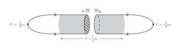
Figure 1: In the degenerate limit $b\to 0$, the two-sphere is deformed into a union of two infinitely stretched cigar-like geometries. The shaded region represents an infinitely long flat cylinder on which the standard $\mathcal{N}=(2,2)$ supersymmetric theories in the Ramond sector are defined.

In the limit $b\to 0$, the sphere gets deformed into a long cylinder with caps at both ends. It can be described as the union of two infinitely stretched cigar geometries attached to each other, as depicted in Fig. 1. In particular, one has a cylinder region arising from zooming near the equator of the squashed two-sphere $S^{2}_{b}$. In order to make this very explicit, it is instructive to change coordinates to $\rho=\tilde{l}\cos\theta$, where the metric of $S^{2}_{b}$ becomes

$$ds^{2}=d\rho^{2}+\left({l\over\tilde{l}}\right)^{2}{\big{(}{\rho/\tilde{l}}\big{)}^{2}\over 1-\big{(}{\rho/\tilde{l}}\big{)}^{2}}d\rho^{2}+l^{2}\left(1-\big{(}{\rho/\tilde{l}}\big{)}^{2}\right)d\varphi^{2}\,.$$ (3.18)

The cylinder metric

$$ds^{2}\simeq d\rho^{2}+l^{2}d\varphi^{2}$$ (3.19)

indeed appears in the region ${\rho/\tilde{l}}\ll 1$ in the limit $b\to 0$, close to the equator of $S^{2}_{b}$. In the cylinder region the spin connection is trivial $\omega\simeq 0$, as expected.

In the flat cylinder region, however, the background connection $V$ for the $U(1)$ $R$-symmetry (2.11) becomes in the limit $b\to 0$

$$V\simeq\frac{1}{2}d\varphi\,.$$ (3.20)

This has important consequences for the boundary conditions of the spinors around the cylinder.

Recall that an antiperiodic spinor $\epsilon(\varphi)$ on a cylinder with coordinates $(\rho,\varphi)$ in the presence of a background flat connection $V=\nu d\varphi$ is equivalent to a spinor with periodicity $\epsilon(\varphi+2\pi)=-e^{2\pi i\nu}\epsilon(\varphi)$ without a background gauge field. Therefore, the background gauge field (3.20) implies that the boundary conditions of the Killing spinors (2.8) on $S^{2}_{b}$ around the cylinder are periodic. Stated differently, the holonomy induced by the background connection $V$ provides the spectral flow changing the states based on the boundary of the cigar from the Neveu-Schwarz sector to the Ramond sector. Consequently the $\mathcal{N}=(2,2)$ gauge theory in the flat cylinder region is in the Ramond sector and on the boundary one has the canonical vacuum $|0\rangle_{\text{R}}$ after the evolution along the infinitely long cylinder.

In short, the background gauge field $V$ (2.11) on the squashed two-sphere allows us to deform the theory on the hemisphere to the theory on the infinitely long cigar geometry in a supersymmetric fashion. The infinite squashing limit $b\to 0$ projects the state based on the boundary of the hemisphere down to the supersymmetric ground state and simultaneously implements the spectral flow to yield the canonical ground state $|0\rangle_{\text{R}}$ in the Ramond sector. Therefore, the path integral on the $S_{b}^{2}$ in the limit $b\to 0$ – which we denoted by $Z_{b}$ – becomes the path integral representation of the overlap ${}_{\text{R}}\langle\bar{0}|0\rangle_{\text{R}}$.

It is noteworthy that, very near the poles, the background gauge field $V$ becomes that required to perform the $A$-twist and $\bar{A}$ twist near the north and south poles respectively. In order to analyze these regions $\theta\simeq 0$ or $\theta\simeq\pi$, we should first choose vielbein that are regular in a patch around each pole. The corresponding spin connection is then given by

$$\omega_{N}=+\left(1-\frac{l\cos\theta}{f(\theta)}\right)d\varphi\ ,\qquad\omega_{S}=-\left(1+\frac{l\cos\theta}{f(\theta)}\right)d\varphi\ .$$ (3.21)

In the infinitely squashed limit $b\to 0$, one can show that

$$V_{N}\simeq\frac{1}{2}\omega_{N}\ ,\qquad V_{S}\simeq-\frac{1}{2}\omega_{S}\ ,$$ (3.22)

which accounts for the A-twisting near the north pole and $\bar{\rm A}$-twisting near the south pole. One can thus say that the theory on the squashed two-sphere nicely interpolates in a supersymmetric manner the A-twisted theory very near the poles with the ${\cal N}=(2,2)$ theory in the R sector on the flat cylinder.

We present a different proof of the conjecture (1.1) in the next section in the context of $\mathcal{N}=(2,2)$ Landau-Ginzburg models on the two-sphere, to which we now turn.

4 Mirror Symmetry and the $S^{2}$ Partition Function

A well established method for computing worldsheet instantons and Gromov-Witten invariants is mirror symmetry. In this approach, initiated in [15], the non-perturbative corrections in Kähler moduli space are captured by a purely geometrical problem in the mirror Calabi-Yau manifold.

In mirror symmetry, the Kähler moduli of a Calabi-Yau get exchanged with the complex structure moduli of the mirror Calabi-Yau. In the language of the GLSM’s, this corresponds to exchanging chiral multiplets and twisted chiral multiplets, which as described earlier, parametrize the complex structure and Kähler moduli respectively.

While no general methods are available to determine the mirror manifold to a given Calabi-Yau, powerful techniques have been developed to compute Gromow-Witten invariants for complete intersections in toric varieties. In the language of GLSM’s, this class of Calabi-Yau manifolds corresponds to gauge theories based on abelian gauge groups. In fact, for abelian GLSM’s describing non-linear sigma models on target spaces with non-negative curvature, Hori and Vafa [12] devised a powerful “dualization” method for obtaining the mirror description of the corresponding sigma models in terms of Landau-Ginzburg models. This includes the mirrors of sigma models on toric varieties and hypersurfaces in toric varieties.

Given that the partition function of $\mathcal{N}=(2,2)$ gauge theories on $S^{2}$ can be computed exactly [6, 7], it is interesting to investigate mirror symmetry from the point of view of the partition function on the two-sphere. This is the goal of this section. By pursuing this line of inquiry, we arrive at an independent proof of the main conjecture (1.1) using Landau-Ginzburg models. Also, pleasingly, we find that the $S^{2}$ partition function of the Hori-Vafa Landau-Ginzburg models [12] exactly reproduce the partition function of the corresponding mirror abelian GLSM’s.

Finally, we consider non-abelian GLSM’s describing complete intersections in Grassmanians, where the dualization methods used [12] are not applicable. Using the exact result for the gauge theory partition function [6, 7], we prove the conjectured mirror description put forward by Hori and Vafa [12].

Before presenting these results, we must first construct the mirror $\mathcal{N}=(2,2)$ supersymmetric Landau-Ginzburg models on the two-sphere $S^{2}$. These theories are written in terms of twisted chiral multiplets since, as mentioned above, mirror symmetry exchanges chiral multiplets, which appear in the GLSM description, with twisted chiral multiplets, which appear in the mirror Landau-Ginzburg description.

4.1 Supersymmetric Twisted Chiral Multiplets on S²

The field content of a twisted chiral multiplet is the same as that of the chiral multiplet. We denote the fields in the twisted chiral multiplet by

$$\text{twisted chiral multiplet}:(Y,\overline{Y},\chi,\bar{\chi},G,\bar{G})\,.$$ (4.1)

The $SU(2|1)$ invariant Lagrangian of a twisted chiral multiplet on the round two-sphere of radius $r$ is given by

$${\cal L}_{\text{twisted}}= D^{i}\overline{Y}D_{i}Y+i\bar{\chi}\gamma^{i}D_{i}\chi+\left(\bar{G}+\frac{\Delta}{r}\overline{Y}\right)\left(G+\frac{\Delta}{r}Y\right)\,.$$ (4.2)

This action is invariant under the supersymmetry transformations given by

$$\delta Y= +i\bar{\epsilon}\frac{1-\gamma^{3}}{2}\chi-i\epsilon\frac{1+\gamma^{3}}{2}\bar{\chi}$$

$$\delta\overline{Y}= -i\bar{\epsilon}\frac{1+\gamma^{3}}{2}\chi+i\epsilon\frac{1-\gamma^{3}}{2}\bar{\chi}\$$

$$\delta\chi= +\gamma^{i}\frac{1+\gamma^{3}}{2}\epsilon D_{i}Y-\gamma^{i}\frac{1-\gamma^{3}}{2}\epsilon D_{i}\overline{Y}-\frac{1+\gamma^{3}}{2}\epsilon\left(\bar{G}+\frac{\Delta}{r}\overline{Y}\right)-\frac{1-\gamma^{3}}{2}\epsilon\left(G+\frac{\Delta}{r}Y\right)\$$

$$\delta\bar{\chi}= +\gamma^{i}\frac{1+\gamma^{3}}{2}\bar{\epsilon}D_{i}\overline{Y}-\gamma^{i}\frac{1-\gamma^{3}}{2}\bar{\epsilon}D_{i}Y+\frac{1+\gamma^{3}}{2}\bar{\epsilon}\left(G+\frac{\Delta}{r}Y\right)+\frac{1-\gamma^{3}}{2}\bar{\epsilon}\left(\bar{G}+\frac{\Delta}{r}\overline{Y}\right)\$$

$$\delta G= -i\bar{\epsilon}\gamma^{i}\frac{1-\gamma^{3}}{2}\nabla_{i}\chi+i\epsilon\gamma^{i}\frac{1+\gamma^{3}}{2}\nabla_{i}\bar{\chi}-i\frac{\Delta}{r}\bar{\epsilon}\frac{1-\gamma^{3}}{2}\chi+i\frac{\Delta}{r}\epsilon\frac{1+\gamma^{3}}{2}\bar{\chi}\$$

$$\delta\bar{G}= -i\bar{\epsilon}\gamma^{i}\frac{1+\gamma^{3}}{2}\nabla_{i}\chi+i\epsilon\gamma^{i}\frac{1-\gamma^{3}}{2}\nabla_{i}\bar{\chi}+i\frac{\Delta}{r}\bar{\epsilon}\frac{1+\gamma^{3}}{2}\chi-i\frac{\Delta}{r}\epsilon\frac{1-\gamma^{3}}{2}\bar{\chi}\,$$ (4.3)

where $\epsilon$ and $\bar{\epsilon}$ are Killing spinors on $S^{2}$. These transformation realize the $SU(2|1)$ algebra off-shell on the twisted chiral multiplet fields. The parameter $\Delta$ can be identified as the Weyl weight of the twisted chiral multiplet. We note that the above Lagrangian and supersymmetry transformations are identical to those of the vector multiplet on $S^{2}$ once various component fields are identified as follows

$$Y=\sigma_{2}+i\sigma_{1}\ ,\qquad\overline{Y}=\sigma_{2}-i\sigma_{1}\ ,\qquad\chi=\lambda\ ,\qquad\bar{\chi}=\bar{\lambda}$$

$$\qquad G={\rm D}-\frac{\sigma_{2}}{r}+iF_{12}\ ,\qquad\bar{G}={\rm D}-\frac{\sigma_{2}}{r}-iF_{12}\ ,$$ (4.4)

and the Weyl weight is fixed to the canonical value, i.e., $\Delta=1$.

Twisted superpotential couplings for the twisted chiral multiplet can be written on $S^{2}$ in an $SU(2|1)$ invariant way in terms of a holomorphic function $W(Y)$. The interaction terms

$${\cal L}_{\text{twisted}}=-iW^{\prime}(Y)\left(G+\frac{\Delta}{r}Y\right)-W^{\prime\prime}(Y)\bar{\chi}\left(\frac{1-\gamma^{3}}{2}\right)\chi+\frac{i}{r}W(Y)\$$ (4.5)

are invariant under the supersymmetry transformations above (4.3). Unlike the superpotential $\mathcal{W}$ couplings for chiral superfields in (2.19), the twisted superpotential $W$ couplings (4.5) are modified in comparison to those in flat space. As we shall show, the deformation term

$$\frac{i}{r}W(Y)$$ (4.6)

in (4.5) controls most of the features of the partition function on the two-sphere even though this term disappears from the action in the flat space, $r\rightarrow\infty$ limit.

Finally, we note that even though twisted chiral multiplets cannot be minimally coupled to conventional vector multiplets, the field strength multiplet $\Sigma$, which is a twisted chiral multiplet, can couple with a twisted chiral multiplet through a twisted superpotential

$$W(\Sigma,Y)\,.$$ (4.7)

In the context mirror symmetry, the coupling of a twisted chiral multiplet $Y$ to $\Sigma$ via a dynamical FI term

$$W(\Sigma,Y)=\Sigma\,Y$$ (4.8)

is known to play an important role [12], and will appear later in our analysis.

Everything that we have discussed for the round two-sphere, admits a fairly simple extension to the squashed two-sphere.

4.2 Landau-Ginzburg Proof of the Conjecture

We first proceed to the computation of the $S^{2}$ partition function of Landau-Ginzburg models by supersymmetric localization. Using the choice of localizing supercharge ${\cal Q}$ in (2.6), the path integral localizes to the saddle point configurations

$$Y=x+iy\ ,\qquad G+\frac{\Delta}{r}Y=0\ ,$$ (4.9)

where $x,y$ are real constants over the two-sphere.

The twisted chiral kinetic terms (4.2) can be shown to be ${\cal Q}$-exact, and thus can be used as the ${\cal Q}$-exact deformation term to compute the one-loop determinant around the saddle points (4.9). The one-loop determinant of a twisted chiral multiplet is trivial, in the sense that it is independent of the choice of saddle point configuration $x$ and $y$.

Therefore, the $S^{2}$ partition function $Z$ of an $\mathcal{N}=(2,2)$ Landau-Ginzburg model with a twisted superpotential $W$ reduces to the following integral

$$Z=\int dYd\overline{Y}e^{-4\pi irW(Y)-4\pi ir\overline{W}(\overline{Y})}=\int dx\,dy\ e^{-4\pi irW(x+iy)-4\pi ir\overline{W}(x-iy)}\,.$$ (4.10)

The partition function depends only on the choice of twisted superpotential $W$.

This computation offers a new way to derive the conjecture in (1.1). We first quickly recall that Landau-Ginzburg models of the type we have discussed capture the physics of non-linear sigma models on Calabi-Yau target space in some regions in Kähler moduli space. This fact can be most elegantly seen using the GLSM description of the Calabi-Yau moduli space. In this framework, the Landau-Ginzburg description corresponds to a different “phase” [1] of the phase diagram parametrized by the Kähler moduli. Furthermore, Landau-Ginzburg models are mirror to GLSM’s describing the nonlinear sigma models on the mirror Calabi-Yau manifold.

Let us now consider a Landau-Ginzburg description of a two dimensional $\mathcal{N}=(2,2)$ superconformal field theory that can appear at a special point in Kähler moduli space. Consider deforming the conformal field theory by exactly marginal operators, which are descendants of operators in the twisted chiral ring. This deformation is implemented in the Landau-Ginzburg description by turning on the twisted superpotential

$$W=i\sum_{a}\tau_{a}\mathcal{O}_{a}(Y)\,,$$ (4.11)

where $\mathcal{O}_{a}(Y)$ are operators in the twisted chiral ring. The parameters $\tau_{a}$ are dimensionless and parametrize the moduli space of the conformal field theory. The partition function on $S^{2}$ is a function of these parameters.

We now differentiate the $S^{2}$ partition function and obtain the following correlation function

$$\partial_{a}\partial_{\bar{b}}\log Z={\left\langle\mathfrak{O}_{a}\cdot\bar{\mathfrak{O}}_{\bar{b}}\right\rangle_{S^{2}}\over Z}\,,$$ (4.12)

where explicitly

$$\mathfrak{O}_{a} =\int d^{2}x\sqrt{g}\ \left(-\partial_{i}{\cal O}_{a}\Big{(}G^{i}+\Delta Y^{i}\right)+{\cal O}_{a}+\text{fermionic terms}\Big{)}$$

$$\bar{\mathfrak{O}}_{\bar{b}} =\int d^{2}x\sqrt{g}\ \Big{(}+\partial_{\bar{j}}\bar{{\cal O}}_{\bar{b}}\left(\bar{G}^{\bar{j}}+\Delta\bar{Y}^{\bar{j}}\right)-\bar{{\cal O}}_{\bar{b}}+\text{fermionic terms}\Big{)}\,.$$ (4.13)

It is important to now note that the operators $\mathfrak{O}_{a}$ and $\bar{\mathfrak{O}}_{\bar{b}}$ are invariant under the supersymmetry transformations (4.3). Therefore, their correlation functions can be computed by the same localization procedure as we did for the $S^{2}$ partition function. Evaluating these operators on the saddle point field configurations (4.9), we find that the two-point correlation function on $S^{2}$ (4.12) can be reduced to the following simple integral

$$\partial_{a}\partial_{\bar{b}}\log Z=-{1\over Z}\int d\vec{x}\,d\vec{y}\ {\cal O}_{a}(\vec{x}+i\vec{y})\bar{{\cal O}}_{\bar{b}}(\vec{x}-i\vec{y})e^{-4\pi iW-4\pi i{\overline{W}}}\ .$$ (4.14)

Let us now consider the insertion of a twisted chiral operator ${\cal O}_{a}$ at the north pole and a twisted anti-chiral operator $\bar{{\cal O}}_{\bar{b}}$ at the south pole of the $S^{2}$. These operators preserve precisely the supercharge ${\cal Q}$ (2.6) with respect to which we have localized the $S^{2}$ partition function. This implies that we can compute this two-point correlation function exactly using the same saddle points. We obtain that

$$\left\langle{\cal O}_{a}(N)\bar{{\cal O}}_{\bar{b}}(S)\right\rangle_{S^{2}}=\int d\vec{x}\,d\vec{y}\ {\cal O}_{a}(\vec{x}+i\vec{y})\bar{{\cal O}}_{\bar{b}}(\vec{x}-i\vec{y})e^{-4\pi iW-4\pi i{\overline{W}}}\ .$$ (4.15)

Comparing the results (4.12) and (4.15) of the two computations we have just performed leads to the following relation

$$-\partial_{a}\partial_{\bar{b}}\log Z=\frac{\left\langle{\cal O}_{a}(N)\bar{{\cal O}}_{\bar{b}}(S)\right\rangle_{S^{2}}}{Z}\ .$$ (4.16)

As shown by Cecotti-Vafa in [11], the two-point correlation function on S² in the r.h.s. of (4.16) turns out to be the normalized ground state metric $G_{a\bar{b}}$ in the space of supersymmetric ground states in the Ramond sector

$$\frac{\left\langle{\cal O}_{a}(N)\bar{{\cal O}}_{\bar{b}}(S)\right\rangle_{S^{2}}}{Z}=\frac{{}_{\text{R}}\langle\bar{b}|a\rangle_{\text{R}}}{{}_{\text{R}}\langle\bar{0}|0\rangle_{\text{R}}}\equiv G_{a\bar{b}}\ .$$ (4.17)

Furthermore, using the $tt^{*}$ equations, it can be proven that [11]

$$G_{a\bar{b}}=-\partial_{a}\partial_{\bar{b}}\ \log\ _{\text{R}}\langle\bar{0}|0\rangle_{\text{R}}\ .$$ (4.18)

Therefore, up to an ambiguity due to Kähler transformations, we arrive at the desired result

$$Z(\tau_{a},\bar{\tau}_{a})=\ _{\text{R}}\langle\bar{0}|0\rangle_{\text{R}}=e^{-\mathcal{K}(\tau_{a},\bar{\tau}_{a})}\ .$$ (4.19)

4.3 Mirror Symmetry and Hori-Vafa Conjecture

Hori and Vafa [12] put forward a powerful method for constructing the mirror description of non-linear sigma models on Kähler manifolds admiting an abelian GLSM description. This method applies to a broad class of Kähler manifolds with non-negative curvature. These authors provide the mirror description of sigma models on toric varieties and hypersurfaces in toric varieties.

In this section we show that the $S^{2}$ partition function of proposed mirror Landau-Ginzburg models and abelian GLSM’s are identical in all cases, even though the expression for their partition functions are rather distinct ((4.10) versus (3.14)). Furthermore, by studying the partition function of non-abelian GLSM’s describing complete intersections in Grassmanians, we prove a conjecture by Hori and Vafa regarding the mirror Landau-Ginzburg description of this interesting class of nonlinear sigma models.

We now consider the partition function of mirror Landau-Ginzburg models for the various cases: toric varieties, hyper surfaces in toric varieties and non-abelian GLSM’s.

Landau-Ginzburg Mirror of Toric Varieties:

For simplicity, we begin with toric varieties based on a GLSM with $U(1)$ gauge group and $n$ chiral multiplets $\Phi_{a}$ with charges $Q_{a}$, where $a=1,2,\ldots,n$. We also start with the case of a GLSM with no superpotential.

According to the Hori-Vafa prescription [12], the dual Landau-Ginzburg description involves a twisted chiral multiplet $\Sigma$, the field strength multiplet constructed from the vector multiplet, and $n$ neutral twisted chiral multiplets $Y^{a}$. The imaginary part of $Y^{a}$ is periodic with period $2\pi$. The mirror Landau-Ginzburg model has a twisted superpotential of the Toda type and the twisted chiral multiplets $Y^{a}$ act as dynamical FI parameters. The explicit twisted superpotential is

$$W=-\frac{1}{4\pi}\left[\Sigma\left(\sum_{a=1}^{n}Q_{a}Y^{a}+2\pi i\tau(\mu)\right)+i\mu\sum_{a=1}^{n}e^{-Y^{a}}\right]\ ,$$ (4.20)

where $\mu$ is an infrared scale, set to be $1/r$ on the two-sphere.

If the original twisted chiral multiplets $\Phi^{a}$ have twisted masses $m_{a}$ and $U(1)_{R}$ charges $-q_{a}$, the mirror Landau-Ginzburg model acquires an extra linear twisted superpotential coupling

$$W_{\text{lin}}=-\frac{1}{4\pi}\sum_{a=1}^{n}\left(m_{a}+i\frac{q_{a}}{2r}\right)Y^{a}\,.$$ (4.21)

In order not to clutter formulas we will mostly focus on the case $m_{a}=0$ and $q_{a}\to 0^{+}$, the later limit arising due to convergence, as will be discussed shortly. Adding it is straightforward and in all cases reproduces the the effect of turning on these parameters on the mirror GLSM.

Using (4.10) and the saddle points of the vector multiplet (3.9), the two-sphere partition function of this Landau-Ginzburg model is given by

$$Z=\sum_{B\in\mathbb{Z}}\int_{-\infty}^{\infty}d\sigma\prod_{a=1}^{n}\int_{-\infty}^{\infty}dx^{a}\int_{-\pi}^{+\pi}dy^{a}\ e^{+2ir\sigma\left(Q_{a}x^{a}-2\pi\xi\right)+iB\left(Q_{a}y^{a}+\vartheta\right)}\cdot e^{2ie^{-x^{a}}\sin y^{a}}\,.$$ (4.22)

Note here that, on the saddle point field configurations, the imaginary part $-\frac{B}{2r}$ of the field strength superfield $\Sigma$ is quantized ($B\in\mathbb{Z}$) while the imaginary part $y^{a}$ of $Y^{a}$ is periodic with period $2\pi$.

Using the integral representation of the Bessel function of the first kind $J_{\alpha}$,

$$J_{\alpha}(x)=\frac{1}{2\pi}\int^{+\pi}_{-\pi}dy\ e^{-i\alpha y}e^{ix\sin y}\ ,$$ (4.23)

we can rewrite the partition function as follows

$$Z=\sum_{B\in\mathbb{Z}}e^{+iB\vartheta}\int d\sigma\ e^{-4\pi ir\sigma\xi}\prod_{a=1}^{n}(-1)^{BQ_{a}}\int dx^{a}\ e^{2ir\sigma Q_{a}x^{a}}J_{BQ_{a}}\left(2e^{-x^{a}}\right)\,.$$ (4.24)

Interestingly, the Fourier transformation of the Bessel function of the first kind with a fine-tuned parameter can be expressed in terms of a ratio of Euler gamma functions

$$\int_{-\infty}^{+\infty}dx\ e^{-qx}e^{2iQpx}J_{BQ}(2e^{-x})=(-1)^{\frac{|BQ|-BQ}{2}}\frac{1}{2}\frac{\Gamma\left(\frac{q}{2}+\frac{1}{2}\left|BQ\right|-iQp\right)}{\Gamma\left(1-\frac{q}{2}+\frac{1}{2}\left|BQ\right|+iQp\right)}\ .$$ (4.25)

This identity holds for all nonzero integer $BQ$ and arbitrary $q$. For $B=0$, one has to be careful about the convergence of the integral. The integral becomes convergent for any positive real $q$. As explained in [6], the physical origin of the divergence at $q=0$ is due to an extra supersymmetric zero mode. Using this formula, we can express the partition function of the Landau-Ginzburg model in the following form

$$Z=\sum_{B\in\mathbb{Z}}e^{+iB\vartheta}\int d\sigma\ e^{-4\pi ir\sigma\xi}\prod_{a=1}^{n}(-1)^{\frac{|BQ_{a}|+BQ_{a}}{2}}\frac{\Gamma\left(\frac{1}{2}\left|BQ_{a}\right|-irQ_{a}\sigma\right)}{\Gamma\left(1+\frac{1}{2}\left|BQ_{a}\right|+irQ_{a}\sigma\right)}\,.$$ (4.26)

This result is in perfect agreement with the two-sphere partition function of the mirror $U(1)$ gauge theory with $n$ chiral multiplets of charge $Q_{a}$ (3.14).

This matching can be easily generalized to GLSM’s with gauge group $G=\prod_{i}U(1)_{j}$ coupled to $n$ chiral multiplets $\Phi^{a}$ carrying charges encoded in the charge matrix $Q^{j}_{a}$. In this case, the twisted superpotential of the mirror Landau-Ginzburg description is given by

$$W=-\frac{1}{4\pi}\bigg{[}\sum_{j=1}^{\text{rk}(G)}\Sigma_{j}\left(\sum_{a=1}^{n}Q_{a}^{j}Y^{a}+2\pi i\tau^{j}(\mu)\right)+i\mu\sum_{a=1}^{n}e^{-Y^{a}}\bigg{]}\ .$$ (4.27)

Extending our previous computation, we find that the two-sphere partition function of this Landau-Ginzburg model can be recast into the following form

$$Z=\sum_{B_{j}\in\mathbb{Z}}e^{+iB_{j}\vartheta^{j}}\int\prod_{j=1}^{\text{rk}(G)}d\sigma_{j}\ e^{-4\pi i\sigma_{j}\xi^{j}}\prod_{a=1}^{n}(-1)^{\frac{\left|B_{j}Q^{j}_{a}\right|+B_{j}Q^{j}_{a}}{2}}\frac{\Gamma\left(\frac{1}{2}\left|B_{j}Q^{j}_{a}\right|-irQ^{j}_{a}\sigma_{j}\right)}{\Gamma\left(1+\frac{1}{2}\left|B_{j}Q^{j}_{a}\right|+irQ^{j}_{a}\sigma_{j}\right)}\,.$$ (4.28)

This exactly reproduces the partition function (3.14) of the mirror GLSM.

Landau-Ginzburg Mirror of Hypersurfaces in Toric Varieties:

Hypersurfaces in toric varieties admit a GLSM description as an abelian gauge theory with a superpotential ${\cal W}$ for the chiral multiplets. As argued in [12], the inclusion of a superpotential in the GLSM does not modify the expression for the twisted superpotential in the mirror Landau-Ginzburg model. There is, nevertheless, an important difference in the Landau-Ginzburg model for the GLSM without and with a superpotential. The choice of fundamental coordinates in the Landau-Ginzburg model changes between the two cases. More precisely, adding superpotential in the GLSM affects the topology of field space in the mirror Landau-Ginzburg model from product of cylinders to product of complex planes with a certain orbifold action. It is therefore interesting to investigate how the two-sphere partition function implements the change of topology of field space after introducing a superpotential term.

For clarity, let us consider the two-sphere partition function of a GLSM with a $U(1)$ gauge group and $n$ chiral multiplets $\Phi^{a}$ with charges $Q_{a}$, where $a=1,2,\ldots,n$. Recall that adding a superpotential $\mathcal{W}$ on the two-sphere in a supersymmetric way is only possible if its $R$-charge is $-2$, so we assign $U(1)$ $R$-charges $-q_{a}$ to the chiral multiplets. The partition function of this theory is (3.14)

$$Z=\sum_{B\in\mathbb{Z}}e^{+iB\vartheta}\int d\sigma\ e^{-4\pi ir\sigma\xi}\prod_{a=1}^{n}(-1)^{\frac{|BQ_{a}|+BQ_{a}}{2}}\frac{\Gamma\left(\frac{q_{a}}{2}+\frac{1}{2}\left|BQ_{a}\right|-irQ_{a}\sigma\right)}{\Gamma\left(1-\frac{q_{a}}{2}+\frac{1}{2}\left|BQ_{a}\right|+irQ_{a}\sigma\right)}\ .$$ (4.29)

Noting that

$$\int_{-\infty}^{+\infty}dx\ e^{-qx}e^{2iQpx}J_{BQ}(2e^{-x})=(-1)^{\frac{|BQ|-BQ}{2}}\frac{1}{2}\frac{\Gamma\left(\frac{q}{2}+\frac{1}{2}\left|BQ\right|-iQp\right)}{\Gamma\left(1-\frac{q}{2}+\frac{1}{2}\left|BQ\right|+iQp\right)}\ ,$$ (4.30)

we can rewrite (4.29) into the following form

$$Z =\sum_{B\in\mathbb{Z}}\int d\sigma\prod_{a=1}^{n}\int dx^{a}e^{-q_{a}x^{a}}\int_{-\pi}^{+\pi}dy^{a}\ e^{+2ir\sigma\left(Q_{a}x^{a}-2\pi\xi\right)+iB\left(Q_{a}y^{a}+\vartheta\right)}e^{2ie^{-x^{a}}\sin y^{a}}$$

$$=\int d\Sigma\,d\bar{\Sigma}\int\left[\prod_{a=1}^{n}dY_{a}d{\overline{Y}}_{a}e^{-\frac{q_{a}}{2}(Y^{a}+{\overline{Y}}^{a})}\right]\ e^{-4\pi irW-4\pi ir\overline{W}}\,,$$ (4.31)

with the twisted superpotential (4.20)

$$W=-\frac{1}{4\pi}\left[\Sigma\left(\sum_{a=1}^{n}Q_{a}Y^{a}+2\pi i\tau(\mu)\right)+i\mu\sum_{a=1}^{n}e^{-Y^{a}}\right]\,.$$ (4.32)

The final expression (4.31) is almost the same as what one obtained in our previous examples with $\mathcal{W}=0$, except for extra weight factors $e^{-\frac{q_{a}}{2}(Y^{a}+{\overline{Y}}^{a})}$ in the measure. Although the dual description involves $n$ twisted chiral multiplets $Y^{a}$ coupled via the same twisted superpotential (4.32), these extra factors are responsible for the subtle difference in choosing what the fundamental variables of the mirror Landau-Ginzburg model are. While a twisted chiral multiplet $Y^{a}$ is the variable dual to a chiral multiplet $\Phi^{a}$ with vanishing $U(1)$ $R$-charge, care must be taken to choose an appropriate dual variable for a chiral multiplet $\Phi^{a}$ of $U(1)$ $R$-charge $q_{a}$. The proper fundamental variable in this case is (no summation over $a$)

$$X_{a}=e^{-\frac{q_{a}}{2}Y^{a}}\ .$$ (4.33)

As we shall now demonstrate, the fundamental Landau-Ginzburg variables (4.33) that naturally arise from the two-sphere partition function of the mirror GLSM (4.31) are in perfect agreement with those proposed by Hori and Vafa [12].

For concreteness, let us consider a degree $n$ hypersurface in $\mathbb{CP}^{n-1}$. For $n=5$, this hypersurface describes the celebrated quintic Calabi-Yau threefold. This Calabi-Yau is described [1] by an abelian GLSM with $n$ chiral multiplets $\Phi^{a}$ of gauge charge $+1$ and a chiral multiplet $P$ of gauge charge $-n$. The superpotential is

$${\cal W}=P\,G_{n}(\Phi_{a})\ ,$$ (4.34)

where $G_{n}$ denotes a homogeneous function of $\Phi^{a}$ of degree $n$. The $R$-charge of $\Phi^{a}$ is $q=2\mathfrak{r}$ while the $R$-charge of $P$ is determined by $q=2-2n\mathfrak{r}$. The parameter $\mathfrak{r}$ can be identified as the gauge charge. Due to the convergence of the integral, this parameter should be in the range of $(0,1/n)$.

Looking at (4.31), the two-sphere partition function of this GLSM can be expressed as

$$Z=\int d\Sigma\,d\bar{\Sigma}\int\prod_{a=1}^{n}\left[dY_{a}d{\overline{Y}}_{a}e^{-\mathfrak{r}(Y_{a}+{\overline{Y}}_{a})}\right]\left[dY_{P}d{\overline{Y}}_{P}e^{-(1-n\mathfrak{r})(Y_{P}+{\overline{Y}}_{P})}\right]\ e^{-4\pi irW-4\pi ir\overline{W}}$$ (4.35)

where the twisted superpotential is given by

$$W=-\frac{1}{4\pi}\bigg{[}\Sigma\left(\sum_{a=1}^{n}Y^{a}-nY_{P}+2\pi i\tau\right)+i\frac{1}{r}\Big{(}\sum_{a=1}^{n}e^{-Y^{a}}+e^{-Y_{P}}\Big{)}\bigg{]}\ .$$ (4.36)

Integration first over $\Sigma,\bar{\Sigma}$ and then over $Y_{P},{\overline{Y}}_{P}$ leads to further simplification of the two-sphere partition function

$$Z=\int\prod_{a}\left[d{\widetilde{X}}_{a}d\overline{{\widetilde{X}}}_{a}\right]\ e^{-W_{\text{eff}}+\overline{W}_{\text{eff}}}\,,$$ (4.37)

where the effective twisted superpotential is

$$W_{\text{eff}}=\sum_{a}{\widetilde{X}}_{a}^{n}+e^{-2\pi i\tau/n}\prod_{a}{\widetilde{X}}_{a}\ .$$ (4.38)

Here the canonical variables ${\widetilde{X}}_{a}$ are given by

$${\widetilde{X}}_{a}=e^{-\frac{1}{n}Y_{a}}\,.$$ (4.39)

Since the imaginary part of the twisted chiral field $Y_{a}$ is periodic with period $2\pi$, we need to identify $\widetilde{X}_{a}\simeq e^{2\pi i/n}\widetilde{X}_{a}$. This implies that the present model is indeed an orbifold of the Landau-Ginzburg with twisted superpotential (4.38). Note that the above choice of fundamental variables is in perfect agreement with the choice proposed in [12].

Landau-Ginzburg Mirror of Nonabelian GLSM’s:

The dualization methods in [12] to derive mirror Landau-Ginzburg models, while very powerful for abelian gauge theories, can not extend to non-abelian gauge theories. On the other hand, the exact computation of the partition function of $\mathcal{N}=(2,2)$ gauge theories on the two-sphere [6, 7] applies to arbitrary gauge theories, and offers a new perspective on the problem of finding the mirror Landau-Ginzburg models to non-abelian GLSM’s. These GLSM’s describe interesting non-linear sigma models on hypersurfaces over the Grassmanian or flag varieties in general, for which no universal method of computation of Gromov-Witten invariants are known.

For concreteness let us consider a $U(N)$ gauge theory coupled to a chiral multiplet in a representation $\mathbf{R}$ of the gauge group. The two-sphere partition function is given by (3.14)

$$Z =\frac{1}{|{\cal W}(G)|}\sum_{B_{j}}e^{+i\vartheta\sum_{j}B_{j}}\int\prod_{j=1}^{\text{rk}(G)}d\sigma_{j}\ e^{-4\pi i\xi\sum_{j}\sigma_{j}}\ \prod_{j<k}\left|\sigma_{j}-\sigma_{k}-i\frac{B_{j}-B_{k}}{2r}\right|^{2}$$

$$\ \ \ \times\prod_{\rho^{j}}(-1)^{\frac{\left|\rho^{j}B_{j}\right|+\rho^{j}B_{j}}{2}}\frac{\Gamma\left(\frac{1}{2}\left|\rho^{j}B_{j}\right|-ir\rho^{j}\sigma_{j}\right)}{\Gamma\left(1+\frac{1}{2}\left|\rho^{j}B_{j}\right|+ir\rho^{j}\sigma_{j}\right)}\,.$$ (4.40)

Here $\rho^{j}$ denote the weights of the representation $\bf R$ of $U(N)$. Using the various identities presented above, we can rewrite the two-sphere partition function of this non-abelian gauge theory in the following form

$$Z =\frac{1}{|{\cal W}(G)|}\sum_{B_{j}}\int\prod_{j=1}^{\text{rk}(G)}d\sigma_{j}\prod_{\rho\in\mathbf{R}}\int dx^{\rho}\int_{-\pi}^{+\pi}dy^{\rho}\ \prod_{j<k}\left|\sigma_{j}-\sigma_{k}-i\frac{B_{j}-B_{k}}{2r}\right|^{2}$$

$$\ \ \ \times e^{+2i\sigma_{j}\left(\rho^{j}x^{\rho}-2\pi\xi\right)+iB_{j}\left(\rho^{j}y^{\rho}+\vartheta\right)}\cdot e^{2ie^{-x^{\rho}}\sin y^{\rho}}\,.$$

This can be further massaged into the following conducive Landau-Ginzburg form

$$Z=\frac{1}{|{\cal W}(G)|}\int\Big{[}\prod_{j=1}^{\text{rk}(G)}d\Sigma_{j}d\bar{\Sigma}_{j}\Big{]}\Big{[}\prod_{\rho\in\mathbf{R}}dY^{\rho}d{\overline{Y}}^{\rho}\Big{]}\prod_{j<k}\left|\Sigma_{j}-\Sigma_{k}\right|^{2}\ e^{-4\pi iW-4\pi i\overline{W}}\,,$$ (4.41)

where the effective twisted superpotential is given by

$$W=-\frac{1}{4\pi}\left[\sum_{j=1}^{\text{rk}(G)}\Sigma_{j}\left(\sum_{\rho\in\mathbf{R}}\rho^{j}Y^{\rho}+2\pi i\tau\right)+i\mu\sum_{\rho}e^{-Y^{\rho}}\right]\ .$$ (4.42)

This result agrees perfectly with the conjectured dual description of this nonabelian GLSM proposed by Hori and Vafa in [12] and follows rather directly from the exact results of the partition function of $\mathcal{N}=(2,2)$ gauge theories on the two-sphere.

5 Discussion

In this paper we have found two physical proofs of the conjecture originally put forward in [10]. This conjecture relates the two-sphere partition function of ${\cal N}=(2,2)$ supersymmetric theories with the Kähler potential $\mathcal{K}$ on the quantum Kähler moduli space of Calabi-Yau manifolds

$$Z(\tau_{a},\bar{\tau}_{a})=e^{-\mathcal{K}(\tau_{a},\bar{\tau}_{a})}\ .$$ (5.1)

One proof uses the invariance of the two-sphere partition function under squashing, which we establish by computing the squashed two-sphere partition function. We then note that this path integral in the infinitely squashed limit represents the overlap of the canonical ground state ${}_{\text{R}}\langle\bar{0}|0\rangle_{\text{R}}$ of the infrared ${\cal N}=(2,2)$ superconformal theory in the Ramond sector defined on a flat cylinder, which indeed computes the Kähler potential $\mathcal{K}(\tau_{a},\bar{\tau}_{a})$. Here the background gauge field needed to define the theory on the squashed two-sphere plays a key role in implementing the spectral flow to the Ramond sector.

Therefore, the partition function on $S^{2}$ of Calabi-Yau GLSM’s offers a new explicit method for computing the Kähler potential and Gromov-Witten invariants in Calabi-Yau sigma models. One advantage of this approach is that it does not discriminate between Calabi-Yau manifolds obtained from abelian and non-abelian Calabi-Yau GLSM’s. This is in stark contrast with other approaches, where powerful, general methods exist for complete intersections in toric varieties – which correspond to abelian gauge theories – but no general methods to compute Gromov-Witten invariants are available otherwise, for example, for Calabi-Yau manifolds based on non-abelian gauge theories. Certain non-abelian GLSM’s for non-complete intersections have been constructed recently [20, 21, 22, 23], and the two-sphere partition function is a new exact method to study them. Indeed, the virtues of the two-sphere partition function approach to Gromov-Witten invariants have already been exposed in [10], where Gromov-Witten invariants for Calabi-Yau manifolds for which no other method is available were computed.

Two dimensional $\mathcal{N}=(2,2)$ theories on the two-sphere can be enriched by adding supersymmetric defects. Among these, line operators localized at the equator appear particularly promising. The simplest such defect is a Wilson loop operator, which was already considered in [6]. It would be interesting to construct domain walls preserving the $SU(1|1)$ symmetry used to localize the $S^{2}$ partition function, and to compute the partition function in the presence of the domain wall, similarly to what was done for domain walls [24] (see also [25]) on the four-sphere [26].

Just as the two-sphere partition function computes worldsheet instantons in a Calabi-Yau, we expect that the $S^{2}$ partition function in the presence of a domain wall to compute woldsheet instanton in the presence of D-branes in the Calabi-Yau geometry. This is a particularly promising speculation since it is notoriously difficult to compute such worldsheet instantons by conventional methods, while the result of the computation of the partition function in the presence of a domain wall will be rather explicit. This may provide a new effective tool to compute open Gromov-Witten invariants in Calabi-Yau geometries.

We have also defined supersymmetric theories for twisted chiral multiplets on the two-sphere, and computed the partition function exactly using localization techniques. Our results have found several interesting applications. Firstly, they provide an alternative proof of the above conjecture in the context of Landau-Ginzburg models. Secondly these results can be used to provide precision studies of mirror symmetry. In particular, our analysis allowed us to show that the partition function of the Landau-Ginzburg models proposed by Hori and Vafa [12] are in exact agreement with the partition function of the mirror GLSM’s. Interestingly, for the case of hypersurfaces in toric varieties, the two-sphere partition function of the GLSM naturally knows what appropriate variables should be used in the mirror Landau-Ginzburg description. The computation of the two-sphere partition function for arbitrary gauge theories provides us with a systematic approach to construct the mirror description of a GLSM with a non-abelian gauge group. This is rather interesting since the usual methods to construct the mirror description break down for non-abelian GLSM’s. As an explicit application, we have used our results to get nontrivial evidence for the mirror description of a certain non-abelian GLSM describing complete intersections in the Grassmannian. The mirror Landau-Ginzburg description we have found proves the conjectured description advanced by Hori and Vafa [12]. It would be interesting to push these ideas as a new tool towards understanding non-abelian dualities in two dimensional gauge theories.

In the GLSM approach to nonlinear sigma models on Kähler manifolds, the isometry group $G_{F}$ of the target space is realized in the GLSM as the flavour symmetry group. Deforming the GLSM by twisted masses $m$, which take values in the Cartan of $G_{F}$, corresponds to adding a supersymmetric potential to the nonlinear sigma model that gauges the corresponding isometries. The nonlinear sigma model in this case computes equivariant Gromov-Witten invariants with respect to the Cartan of $G_{F}$. In this context the twisted masses map to the equivariant parameters. In these theories, the partition function of the GLSM on the (squashed) two-sphere is a non-trivial function of the twisted masses. It would be interesting to explore in detail the two-sphere partition function for these theories as a method for extracting equivariant Gromov-Witten invariants.

In [6][7] it was shown that the two-sphere partition function of gauge theories admit both a Coulomb branch and Higgs branch representation. In the first representation the partition function is written as an integral over the Coulomb branch, while in the Higgs branch representation the partition function is expressed as a sum over Higgs vacua of the product of vortex and anti-vortex partition functions. We expect – in specific examples – a similar dual description of the partition function of Landau-Ginzburg models with a twisted superpotential $W$. We have shown that the partition function of such theories is given by the following integral

$$Z=\int dYd\overline{Y}e^{-4\pi irW(Y)-4\pi ir\overline{W}(\overline{Y})}\,.$$ (5.2)

In section 4 we have demonstrated in examples how this integral reproduces the “Coulomb branch” representation of the mirror gauge theory. The “Higgs branch” representation of the partition function (5.2) as a sum of the product of a holomorphic and an anti-holomorphic function of the parameters in the twisted superpotential, can be obtained by decomposing the integral as a sum over integration cycles, which depend on the critical points of the twisted superpotential $W$. These methods have been recently used by Witten [27] and Gaiotto and Witten [28] in the context of analytic continuation of Chern-Simons theory.

The partition function on the squashed two-sphere can be enriched both by introducing twisted mass terms and by inserting twisted chiral operators at the north pole and twisted antichiral operators at the south pole. This follows from the fact that twisted mass terms and these operator insertions at the poles respect the supercharge $\mathcal{Q}$ with which we localized the path integral. It would be particularly interesting to explore the relation between this enriched two-sphere partition function and the ground state metric in the $tt^{*}$ formulation for massive theories [11], with an emphasis on possible applications to the wall-crossing phenomena of BPS kinks [29].

Along a similar line of inquiry, it would also be interesting to generalize the ideas presented above to four dimensional $\mathcal{N}=2$ gauge theories, as these theories realize many of the same phenomena we have discussed in the context of two dimensional $\mathcal{N}=(2,2)$ theories.

Acknowledgement

We would like to thank Stefano Cremonesi, Nima Doroud, Davide Gaiotto and Bruno Le Floch for valuable discussions. We thank the Simons Center for Geometry and Physics for hospitality, where this work was initiated and completed, and where a preliminary version of these results was presented. S.L. would like to thank Aspen Center for Physics (NSF Grant No. 1066293) for hospitality. Research at the Perimeter Institute is supported in part by the Government of Canada through NSERC and by the Province of Ontario through MRI. J.G. also acknowledges further support from an NSERC Discovery Grant and from an ERA grant by the Province of Ontario. The work of S.L. is supported by the Ernest Rutherford fellowship of the Science & Technology Facilities Council ST/J003549/1.

Appendix

Appendix A Details of the Computation

We present in this section the details of the one-loop determinant computations.

Our choice of supercharge ${\cal Q}$ is exactly the same to what is chosen for the round two-sphere, which generates the $SU(1|1)$ supersymmetry algebra. The Killing spinors associated to this supercharge ${\cal Q}$ are denoted by $\epsilon_{\cal Q}$ and ${\bar{\epsilon}}_{\cal Q}$, normalized such that

$${\bar{\epsilon}}_{\cal Q}\gamma^{3}\epsilon_{\cal Q}=1\ .$$ (A.1)

From now on, we ignore the subscript ${\cal Q}$ unless it causes any confusions. Denoting the rests of bi-linear forms as

$$w=\bar{\epsilon}\epsilon\ ,\qquad v^{i}=\bar{\epsilon}\gamma^{i}\epsilon\ ,$$ (A.2)

it is easy to show that they satisfy the following relations frequently used in what follows

$$w^{2}-v_{i}v^{i}=1\ ,\qquad v_{i}\bar{\epsilon}\gamma^{i}+\bar{\epsilon}\gamma^{3}=w\bar{\epsilon}\ ,\qquad v_{i}\gamma^{i}\epsilon+\gamma^{3}\epsilon=w\epsilon\ ,$$ (A.3)

and

$$\gamma^{i}D_{i}w=\frac{1}{f}\gamma^{3}\gamma^{i}v_{i}\ ,\qquad D_{i}v^{i}=0\ ,\qquad\gamma^{ij}D_{i}v_{j}=\frac{2}{f}w\gamma^{3}\ ,\qquad v^{i}\partial_{i}f=0\ .$$ (A.4)

The following identities is also useful

$$\frac{1}{4}\Big{(}{\cal R}+2iG_{ij}\gamma^{ij}\Big{)}\epsilon =\Big{(}\frac{1}{2f^{2}}-\frac{1}{2}\gamma^{i}\gamma^{3}\partial_{i}f^{-1}\Big{)}\epsilon\ ,$$

$$\frac{1}{4}\bar{\epsilon}\Big{(}{\cal R}+2iG_{ij}\gamma^{ij}\Big{)} =\bar{\epsilon}\Big{(}\frac{1}{2f^{2}}-\frac{1}{2}\gamma^{i}\gamma^{3}\partial_{i}f^{-1}\Big{)}\ ,$$ (A.5)

where $G=dV$.

It would be tedious to work out all the eigenmodes. Limited to the one-loop determinant, it is in fact not necessary to know the explicit expressions of all the eigenmodes and their eigenvalues. This is due to the vast cancellation between the contributions to the one-loop determinant from bosonic and fermionic modes thanks to supersymmetry. It is therefore sufficient to understand how this cancellation happens.

A.1 Matter Multiplet

First, we consider the one-loop determinant from a chiral multiplet of R-charge $-q$ and gauge charge one, coupled to an abelian vector multiplet. It turns out that, instead of the original Lagrangian (2.18), a different choice of a ${\cal Q}$-exact deformation simplifies the one-loop determinant computation. We choose the regulator Lagrangian as follows

$${\cal L}_{\text{reg}}=-\delta_{\epsilon}\delta_{\bar{\epsilon}}\left(\bar{\psi}\gamma^{3}\psi-2\bar{\phi}\sigma_{2}\phi\right)\ ,$$ (A.6)

which leads to the kinetic operators $\Delta_{b}$ and $\Delta_{f}$

$$\Delta_{b} =-D_{i}^{2}+\sigma_{1}^{2}+\sigma^{2}+\frac{q}{4}{\cal R}+\frac{q-1}{f}v^{i}D_{i}+\frac{q-1}{f}w\sigma_{1}+\frac{q^{2}-2q}{4f^{2}}\ ,$$

$$\Delta_{f} =-i\gamma^{i}D_{i}+i\sigma_{1}-\sigma\gamma^{3}-i\frac{1}{2f}\gamma^{3}+i\frac{q-1}{2f}v_{i}\gamma^{i}+i\frac{q-1}{2f}w\ ,$$ (A.7)

acting on scalars and fermions of R-charges $-q$ and $1-q$, respectively. Here $\sigma_{1}$ and the background gauge field $A$ involved in the covariant derivative are given by (3.7). For simplicity, it is also useful to consider spinor eigenmodes for an operator defined by

$$\gamma^{3}\Delta_{f}\Psi=M\Psi\ ,$$ (A.8)

rather than those for the original one.

super multiplet

Given such a spinor eigenmode $\Psi$ for $\gamma^{3}\Delta_{f}\doteq M$, it is straightforward to show that

$$\Phi=\bar{\epsilon}\Psi\$$ (A.9)

is a scalar eigenmode for $\Delta_{b}\doteq-M(M+2\sigma)$. Secondly, let $\Phi$ denote a scalar eigenmode for $\Delta_{b}\doteq-M(M+2\sigma)$. Defining a pair of spinors as

$$\Psi_{1}=\gamma^{3}\epsilon\Phi\ ,\qquad\Psi_{2}=i\gamma^{i}\epsilon D_{i}\Phi+i\epsilon\sigma_{1}\Phi+\gamma^{3}\epsilon\left(\sigma\Phi+i\frac{q}{2f}\right)\Phi\ ,$$ (A.10)

one can show that $\gamma^{3}\Delta_{f}$ can act on them as follows

$$\gamma^{3}\Delta_{f}\begin{pmatrix}\Psi_{1}\\ \Psi_{2}\end{pmatrix}=\begin{pmatrix}-2\sigma&1\\ M(M+2\sigma)&0\end{pmatrix}\begin{pmatrix}\Psi_{1}\\ \Psi_{2}\end{pmatrix}\ .$$ (A.11)

The matrix on the right hind side has eigenvalues

$$\gamma^{3}\Delta_{f}\doteq M\ ,\ \ -(M+2\sigma)\ .$$ (A.12)

We thus found a pair between a scalar eigenmode with $\Delta_{b}\doteq-M(M+2\sigma)$ and two spinor eigenmodes with $\gamma^{3}\Delta_{f}\doteq M,-(M+2\sigma)$. The map pairing scalar and spinor eigenmodes could be guessed from the SUSY variation rules (2.17).

Due to the cancellation, the contribution to the one-loop determinant from any modes participating in this pairing becomes trivial. There are two types of eigenmodes which provide nontrivial contribution to the one-loop determinant, which fail to fall into the aforementioned multiplet structure. That is to say, either the map (A.9) or the map (A.10) becomes ill-defined.

unpaired spinor eigenmodes

We start with the unpaired spinor egenmodes which vanish when contracted with $\bar{\epsilon}$. As consequence, these modes do not have scalar partners. They take the following form

$$\Psi=\bar{\epsilon}g(\theta,\varphi)\ ,$$ (A.13)

where $g(\theta,\varphi)$ is a scalar of R-charge $2-q$ and of gauge charge $+1$. Then, the eigenmode equation $\Delta_{f}\Psi=\gamma^{3}M\Psi$ gives us

$$-i\gamma^{i}\bar{\epsilon}D_{i}g+i\sigma_{1}\bar{\epsilon}g=\left(M+\sigma_{2}+i\frac{q-2}{2f}\right)\gamma^{3}\bar{\epsilon}g$$ (A.14)

with the covariant derivative defined by

$$Dg=d-i\frac{B}{2}\left(\kappa-\cos\theta\right)d\varphi+i\frac{q-2}{2}\left(1-\frac{l}{f}\right)d\varphi\ ,\qquad\sigma_{1}=-\frac{B}{2l}\ .$$ (A.15)

It leads to the following two equations

$$\partial_{\varphi}g=-\left(Ml+\sigma l+i\frac{q-2}{2}-i\frac{B\kappa}{2}\right)g\ ,$$ (A.16)

and

$$\frac{-i}{f}\partial_{\theta}g+\frac{\cos\theta}{\sin\theta}\left(M+\sigma+i\frac{q-2}{2f}\right)g+\frac{i}{\sin\theta}\sigma_{1}g=0\ .$$ (A.17)

Assuming $g(\theta,\varphi)=e^{-iJ\varphi}h(\theta)$, the first equation (A.16) determines the eigenvalue $M$,

$$iJ=\left(Ml+\sigma l+i\frac{q-2}{2}-i\frac{B\kappa}{2}\right)\ ,$$ (A.18)

while the second equation (A.17) determines the function $h(\theta)$,

$$\frac{-i}{f}\partial_{\theta}h+\frac{\cos\theta}{\sin\theta}\left(i\frac{J}{l}-i\frac{q-2}{2l}+i\frac{q-2}{2f}+i\frac{B\kappa}{2l}\right)h-\frac{i}{\sin\theta}\frac{B}{2l}h=0\ .$$ (A.19)

It is not important to know the precise expression of the solutions to the above differential equation. All we need to care about is when the solution becomes non-normalizable. Looking at the differential equation, the solution can develop singularities at the north pole $\theta=0$ and the south pole $\theta=\pi$. One can easily show that the solutions near the pole are approximate to

$$h(\theta)\sim\sin^{J}\theta\ ,$$ (A.20)

For the normalizability, one needs to require $J$ to be non-negative. As a consequence, the eigenvalues for unpaired spinors eigenmodes are given by

$$Ml=i\left(J+1+i\sigma l-\frac{q}{2}+\frac{|B|}{2}\right)\ ,$$ (A.21)

where $J\geq 0$.

missing spinor eigenmodes

Other pieces contributing to the one-loop determinant arise from the missing spinor eigenmodes. It happens when the map (A.10) does not provide two independent spinor eigenmodes from a single scalar eigenmode $\Phi$. In other words, $\Psi_{1}=-M\Psi_{2}$ for a constant $M$. One can show that $\Psi_{1}=-M\Psi_{2}$ is indeed a spinor eigenmode,

$$\gamma^{3}\Delta_{f}\Psi_{1}=-2\sigma_{2}\Psi_{1}+\Psi_{2}=-\left(M+2\sigma_{2}\right)\Psi_{1}\ .$$ (A.22)

Note that any scalar function $\Phi$ of R-charge $-q$ satisfying the relation below

$$\Psi_{1}=-M\Psi_{2}\ \to\ -i\gamma^{i}\epsilon D_{i}\Phi-i\sigma_{1}\epsilon\Phi=\gamma^{3}\epsilon\left(M+\sigma_{2}+i\frac{q}{2f}\right)\Phi\ ,$$ (A.23)

is guaranteed to be a scalar eigenmode for $\Delta_{b}\doteq-M(M+2\sigma_{2})$ via the map $\bar{\epsilon}\Psi_{1}$ (A.9). Hence, a spinor eigenmode for $\Delta_{f}\doteq M$ is missing, which results in the $\frac{1}{M}$ factor for the one-loop determinant. The equation (A.23) can be managed into the following two equations

$$\partial_{\varphi}\Phi=-\left(Ml+\sigma l+i\frac{q}{2}-i\frac{B\kappa}{2}\right)\Phi\ ,$$ (A.24)

and

$$\frac{-i}{f}\partial_{\theta}\Phi-\frac{\cos\theta}{\sin\theta}\left(M+\sigma+i\frac{q}{2f}\right)\Phi-\frac{i}{\sin\theta}\sigma_{1}\Phi=0\ .$$ (A.25)

Assuming $\Phi(\theta,\varphi)=e^{+iJ\varphi}\chi(\theta)$, the first equation (A.24) determines the eigenvalue $M$,

$$iJ=-\left(Ml+\sigma l+i\frac{q}{2}-i\frac{B\kappa}{2}\right)\ ,$$ (A.26)

while the second equation (A.25) determines the unknown function $\chi(\theta)$,

$$\frac{-i}{f}\partial_{\theta}\chi+\frac{\cos\theta}{\sin\theta}\left(i\frac{J}{l}+i\frac{q}{2l}-i\frac{q}{2f}-i\frac{B\kappa}{2l}\right)\chi+\frac{i}{\sin\theta}\frac{B}{2l}\chi=0\ .$$ (A.27)

Again, it is enough to know the normalizability of the solutions. Looking at the differential equation, the solution can develop singularities at the north pole $\theta=0$ and the south pole $\theta=\pi$. One can easily show that the solutions near the pole are approximate to

$$\chi(\theta)\sim\sin^{J}\theta\ ,$$ (A.28)

For the normalizability, one needs to require $J$ to be non-negative. Consequently, the eigenvalues for unpaired spinors eigenmodes are given by

$$Ml=-i\left(J-i\sigma_{2}l+\frac{q}{2}+\frac{|B|}{2}\right)\ ,$$ (A.29)

where $J\geq 0$.

one-loop determinant

For a given superselection sector $B$, collecting all the results (A.21) and (A.29) results in

$$\left.\frac{\text{det}\Delta_{f}}{\text{det}\Delta_{b}}\right|_{B} \simeq\left.\frac{\text{det}\gamma^{3}\Delta_{f}}{\text{det}\Delta_{b}}\right|_{B}$$

$$\simeq\prod_{J=0}^{\infty}\frac{J+1+i\sigma l-\frac{q}{2}+\frac{|B|}{2}}{J-i\sigma l+\frac{q}{2}+\frac{|B|}{2}}\ ,$$ (A.30)

where the symbol ‘$\simeq$’ represents the equality up to a sign factor independent of the vacuum expectation value $\sigma$ but dependent on the flux $B$. One can fix this factor from the comparison to the result for the round-sphere [6, 7]. That is to say, the sign factor is determined by $(-1)^{\frac{|B|+B}{2}}$. This result is exactly the same to the result for the round two-sphere.

A.2 Vector Multiplet

Let us now in turn consider the one-loop determinant from the vector multiplet. We denote the fluctuation modes for the vector and scalar fields as follows

$$A=\frac{B}{2}\left(\kappa-\cos\theta\right)d\varphi+a\ ,\qquad\sigma_{1}=-\frac{B}{2l}+\zeta\ ,\qquad\sigma_{2}=\sigma+\eta\ .$$ (A.31)

With the Cartan-Wyel basis ($E_{\pm\alpha},H$) where $\alpha$ denote the positive roots of G, all the adjoint fields $\varphi$ can be decomposed as

$$\varphi=\sum_{i=1}^{r}\varphi^{i}H_{i}+\sum_{\alpha\in\Delta^{+}}\left(\varphi^{\alpha}E_{\alpha}+\varphi^{-\alpha}E_{-\alpha}\right)\ .$$ (A.32)

The contribution from the modes $\varphi^{i}$ to the one-loop determinant is $\sigma$-independent and one can therefore ignore them in the discussion below. One can show that the Laplacian operators action on bosonic fluctuations $(a^{\alpha},\eta^{\alpha},\zeta^{\alpha})$ takes the following form

$$\Delta=\begin{pmatrix}-\ast D\ast D+(\alpha\cdot\sigma)^{2}+\frac{\mathfrak{q}^{2}}{l^{2}}&-i(\alpha\cdot\sigma)D&i\frac{\mathfrak{q}}{l}D-\ast D\frac{1}{f}\\ -i(\alpha\cdot\sigma)\ast D\ast&-\ast D\ast D+\frac{\mathfrak{q}^{2}}{l^{2}}&(\alpha\cdot\sigma)\frac{\mathfrak{q}}{l}\\ i\frac{\mathfrak{q}}{l}\ast D\ast+\frac{1}{f}\ast D&(\alpha\cdot\sigma)\frac{\mathfrak{q}}{l}&-\ast D\ast D+(\alpha\cdot\sigma)^{2}+\frac{1}{f^{2}}\end{pmatrix}\ ,$$ (A.33)

where $\mathfrak{q}=\frac{\alpha\cdot B}{2}$ for $\alpha\in\Delta$.

non-physical modes

One can easily find two eigenvectors $(a^{\alpha},\eta^{\alpha},\zeta^{\alpha})$ of the operator $\Delta$,

$$\Delta\doteq 0: \ \ (iD\eta,\ (\alpha\cdot\sigma)\eta,\ -\frac{\mathfrak{q}}{l}\eta)$$

$$\Delta\doteq\Delta_{0}+(\alpha\cdot\sigma)^{2}: \ \ (-i(\alpha\cdot\sigma)D\eta,\ \Delta_{0}\eta,\ \frac{\mathfrak{q}}{l}(\alpha\cdot\sigma)\eta)\ ,$$ (A.34)

where $\Delta_{0}$ denotes an eigenvalue of an operator ‘$-\ast D\ast D+\frac{\mathfrak{q}^{2}}{l^{2}}$’. Obviously, the zero eigenmodes of $\Delta$ corresponds to gauge symmetry which should not be regarded as physical modes. In order to evaluate the path integral properly, one needs to take into account for the Faddeev-Popov determinant. We however choose a rather short-cut discussed in [13], instead of considering the ghost fields and some modifications on supersymmetry by BRST transformtaion. One can show that the contribution from another eigenmodes in (A.34) for $\Delta\doteq\Delta_{0}+(\alpha\cdot\sigma)^{2}$ is exactly canceled by the Faddeev-Popov determinant,

$$1={\cal J}\cdot\int D^{\prime}w\ \text{Exp}\Big{[}-\frac{1}{2}\int\ \text{tr}\left(w\wedge\ast\big{(}-\ast D\ast D+\frac{\mathfrak{q}^{2}}{l^{2}}+(\alpha\cdot\sigma)^{2}\big{)}w\right)\Big{]}\ ,$$ (A.35)

which arises from the gauge fixing excluding the contribution from zero eigenvalues. For details, please refer to [13].

super multiplet

The four bosonic eigenmodes for ($a^{\alpha},\eta^{\alpha},\zeta^{\alpha}$) split into two covariant longitudinal-modes with $a^{\alpha}\sim D\eta^{\alpha}$ and two transverse modes with $a^{\alpha}\sim\ast D\eta^{\alpha}$. As explained above, the covariant longitudinal-modes results in no net contribution to the one-loop determinant. The problem is therefore how two phsyical bosonic-modes can be paired with the spinor eigenmdes.

Fixing a gauge,

$$\ast D\ast a^{\alpha}=-i\frac{\mathfrak{q}}{l}\zeta^{\alpha}\ ,\qquad\eta^{\alpha}=0\ ,$$ (A.36)

the differential operators of our interest under the gauge choice (A.36) become

$$\Delta_{b} =\begin{pmatrix}-\ast D\ast D+(\alpha\cdot\sigma)^{2}+\frac{\mathfrak{q}^{2}}{l^{2}}&i\frac{\mathfrak{q}}{l}D-\ast D\frac{1}{f}\\ i\frac{\mathfrak{q}}{l}\ast D\ast+\frac{1}{f}\ast D&-\ast D\ast D+\frac{1}{f^{2}}+(\alpha\cdot\sigma)^{2}\end{pmatrix}\ ,$$

$$\Delta_{f} =i\gamma^{i}D_{i}-i\frac{\mathfrak{q}}{l}+(\alpha\cdot\sigma)\gamma^{3}\ ,$$ (A.37)

where the operator $\Delta_{b}$ acts on $(a^{\alpha},\zeta^{\alpha})$. For later convenience, it is useful to consider the eigenmodes for the following operators,

$$\delta_{b}\equiv\begin{pmatrix}i(\alpha\cdot\sigma)+i\frac{\mathfrak{q}}{l}\ast&-\ast D\\ \ast D&\frac{1}{f}+i(\alpha\cdot\sigma)\end{pmatrix}\ ,\qquad\gamma^{3}\Delta_{f}\ .$$ (A.38)

One can show that, for any eigenmode of $\delta_{b}\doteq-iM$,

$$\delta_{b}\delta_{b}=\Delta_{b}+2i(\alpha\cdot\sigma)\delta_{b}\ \to\ \Delta_{b}\doteq-M\big{(}M+2(\alpha\cdot\sigma)\big{)}\ .$$ (A.39)

It implies that

$$\det\Delta_{b}=\left(\det\delta_{b}\right)^{2}\ .$$ (A.40)

For the vector multiplet, the bosonic and sermonic eigenmodes can be paired in the following manner. Let $({\cal A},\Sigma)$ denote a vector/scalar eigenmode for $\delta_{b}\doteq-iM$. A spinor eigenmode for $\gamma^{3}\Delta_{f}\doteq-M$ can be obtained from the map below

$$\Lambda=\left(\gamma^{3}\gamma^{i}{\cal A}_{i}+i\Sigma\gamma^{3}\right)\epsilon\ .$$ (A.41)

On the other hand, the map from a spinor eigenmode for $\gamma^{3}\Delta_{f}\doteq-M$ to a vector/scalar eigenmode for $\delta_{b}\doteq-iM$ is

$${\cal A}=-i\left(M+\alpha\cdot\sigma\right)\bar{\epsilon}\gamma_{i}\Lambda e^{i}-D\left(\bar{\epsilon}\gamma^{3}\Lambda\right)\ ,$$

$$\Sigma=\left(M+\alpha\cdot\sigma\right)\bar{\epsilon}\Lambda-i\frac{\mathfrak{q}}{l}\bar{\epsilon}\gamma^{3}\Lambda\ .$$ (A.42)

The relation could be guessed from the supersymmetry transformation laws (2.12) with some care given to the gauge condition (A.36). Any paired modes via the above maps are irrelevant when computing the one-loop determinant. As in the case for the matter multiplet, one can have nontrivial contribution to the one-loop determinant from unpaired and missing spinor eigenmodes.

unpaired spinor eigenmodes

Unpaired spinor eigenmodes are annihilated by the map (A.42): one can first show that

$$\Sigma=0\ \to\ \Lambda=g(\theta,\varphi)\left(\bar{\epsilon}+\frac{i\mathfrak{q}}{l\left(M+\alpha\cdot\sigma\right)}\gamma^{3}\bar{\epsilon}\right)\ .$$ (A.43)

Using the above expression for $\Lambda$, one needs to satisfy the condition ${\cal A}=0$ and the spinor eigenmode equation $\gamma^{3}\Delta_{f}\Lambda=-M\Lambda$ simultaneously. At first, it looks overdetermined but it turns out that one relation implies another. One can show that the undetermined function $g(\theta,\varphi)$ should satisfy

$$\partial_{\varphi}g-ig-i\mathfrak{q}\kappa g+l\left(M+\alpha\cdot\sigma\right)g=0\ ,$$ (A.44)

and

$$\frac{1}{f}\sin\theta\partial_{\theta}g+\cos\theta\left(\frac{1}{f}+i\left(M+\alpha\cdot\sigma\right)\right)g+\frac{\mathfrak{q}}{l}g=0\ .$$ (A.45)

Using the ansatz $g(\theta,\varphi)=e^{-iJ\varphi}h(\theta)$, the first equation (A.44) determines the eigenvalues $M$

$$Ml=+i\left(J+1+\mathfrak{q}\kappa+i\alpha\cdot\sigma l\right)\ .$$ (A.46)

Solving the second equation (A.45) determines the function $h(\theta)$

$$\frac{1}{f}\sin\theta\partial_{\theta}h+\cos\theta\left(\frac{1}{f}-\frac{J+1+\mathfrak{q}\kappa}{l}\right)h+\frac{\mathfrak{q}}{l}h=0\ .$$ (A.47)

It is enough to know when the solution becomes normalizable. Near the poles $\theta=0,\pi$, the solutions are approximate to

$$h(\theta)\sim\sin^{J}\theta\ .$$ (A.48)

Naively, the normalizablity could imply that $J$ is non-negative. However, with a careful look at (A.43), one can show that the eigenmode of $J=-1$, i.e., $l\left(M+\alpha\cdot\sigma\right)=i|\bf q|$, are indeed normalizable. We have the following cases:

1. for the positive $\mathfrak{q}>0$, the spinor eigenmode (A.43) of $J=-1$ (or equivalently $\kappa=1$), would-be-singular at the north pole, becomes

   $$\Lambda\sim\begin{pmatrix}\frac{1}{\cos\frac{\theta}{2}}\\ 0\end{pmatrix}\ ,$$ (A.49)

   which is smooth at the north pole $\theta=0$.

2. for the negative $\mathfrak{q}<0$, the spinor eigenmode (A.43) of $J=-1$ (or equivalently $\kappa=-1$), would-be-singular at the south pole, becomes

   $$\Lambda\sim\begin{pmatrix}0\\ \frac{1}{\sin\frac{\theta}{2}}\end{pmatrix}\ ,$$ (A.50)

   which is smooth at the south pole $\theta=\pi$.

3. One remark is that such modes of $J=-1$ become non-normalizable when $B=0$.

As a summary, the eigenvalues for unpaired spinor eigenmodes are given by

$$Ml =+i\Big{(}J+|\mathfrak{q}|+i\alpha\cdot\sigma l\Big{)}\ \ \text{ for }B\neq 0\ ,$$

$$Ml =+i\Big{(}J+1+i\alpha\cdot\sigma l\Big{)}\ \ \ \ \text{ for }B=0\ ,$$ (A.51)

where $J\geq 0$.

missing spinor eigenmodes

In order to work out the missing spinor eigenmodes, one begins by solving ${\cal A}_{i}\gamma^{3}\gamma^{i}\epsilon+i\Sigma\gamma^{3}\epsilon=0$. It leads to

$${\cal A}=g(\theta,\varphi)\left(e^{1}+i\cos\theta e^{2}\right)\ ,\ \ \Sigma=ig(\theta,\varphi)\sin\theta\ .$$ (A.52)

Using the above expression for $({\cal A},\Sigma)$, one needs to satisfy the eigenmode equations $\delta_{b}\doteq-iM$ and the gauge condition (A.36) simultaneously. At first, it again looks overdetermined but turns out that any solutions to one of the eigenmode equation with the ansatz (A.52),

$$\ast D{\cal A}+\left(\frac{1}{f}+i(M+\alpha\cdot\sigma)\right)\Sigma=0\ ,$$ (A.53)

automatically satisfy the other relations. That is to say, it is sufficient to solve the following two equations

$$\partial_{\varphi}g+\Big{(}l(M+\alpha\cdot\sigma)-i\mathfrak{q}\kappa\Big{)}g=0\ ,$$ (A.54)

and

$$\frac{1}{f}\Big{(}\sin\theta\partial_{\theta}+\cos\theta\Big{)}g-\frac{\mathfrak{q}}{l}g-i\cos\theta\left(M+\alpha\cdot\sigma\right)g=0\ .$$ (A.55)

Putting the ansatz $g(\theta,\varphi)=e^{+i(J+1)\varphi}h(\theta)$, the first equation (A.54) determines the eigenvalue $M$,

$$Ml=-i\Big{(}J+1-\mathfrak{q}\kappa-i\alpha\cdot\sigma l\Big{)}\ .$$ (A.56)

The second equation which determines the function $h(\theta)$ can be rewritten as

$$\frac{1}{f}\sin\theta\partial_{\theta}h+\frac{1}{f}\cos\theta h-\frac{\mathfrak{q}}{l}h-\cos\theta\left(\frac{J+1-\mathfrak{q}\kappa}{l}\right)h=0\ .$$ (A.57)

Again, one can show that near the poles $\theta=0,\pi$ the solutions are approximate to

$$h(\theta)\sim\sin^{J}\theta\ .$$ (A.58)

For the normalizablility, one needs to require $J$ to be non-negative. As a summary, the eigenvalue for missing spinor eigenmodes are given by

$$Ml=-i\Big{(}J+1+|\mathfrak{q}|-i\alpha\cdot\sigma l\Big{)}\ ,$$ (A.59)

where $J\geq 0$.

one-loop determinant

For a given superselection sector $B\neq 0$, the contribution to the one-loop determinant from the vector multiplet results in

$$\left.\frac{\det\Delta_{f}}{\sqrt{\det\Delta_{b}}}\right|_{B\neq 0} \simeq\left.\frac{\det\gamma^{3}\Delta_{f}}{\det\delta_{b}}\right|_{B\neq 0}$$

$$\simeq\prod_{\alpha\in\Delta_{\text{root}}}\prod_{J=0}\frac{J+\left|\frac{\alpha\cdot B}{2}\right|-i(\alpha\cdot\sigma l)}{J+1+\left|\frac{\alpha\cdot B}{2}\right|+i(\alpha\cdot\sigma l)}$$

$$\simeq\prod_{\alpha\in\Delta_{+}}\Bigg{[}(\alpha\cdot\sigma l)^{2}+\left(\frac{\alpha\cdot B}{2}\right)^{2}\Bigg{]}\ .$$ (A.60)

By comparing the above results to those in the round-sphere, one can fix a $\sigma-$independent factor by the unity. In the sector of $B=0$, one gets the trivial result for the one-loop determinant. The result is the same to the result for the round two-sphere [6, 7].

References

- [1] E. Witten, “Phases of N = 2 theories in two dimensions,” Nucl. Phys. B403 (1993) 159–222, hep-th/9301042.
- [2] L. J. Dixon, “Some world-sheet properties of superstring compactifications, on orbifolds and otherwise,” Lectures at the 1987 ICTP summer Workshop in High Energy Physics and Cosmology (1987).
- [3] W. Lerche, C. Vafa, and N. P. Warner, “Chiral Rings in N=2 Superconformal Theories,” Nucl.Phys. B324 (1989) 427.
- [4] M. Gromov, “Pseudoholomorphic curves in symplectic manifolds,” Invent.Math. 82 (1985) 307–347.
- [5] E. Witten, “Topological Sigma Models,” Commun.Math.Phys. 118 (1988) 411.
- [6] N. Doroud, J. Gomis, B. Le Floch, and S. Lee, “Exact Results in D=2 Supersymmetric Gauge Theories,” 1206.2606.
- [7] F. Benini and S. Cremonesi, “Partition functions of ) gauge theories on and vortices,” 1206.2356.
- [8] D. R. Morrison and M. R. Plesser, “Summing the instantons: Quantum cohomology and mirror symmetry in toric varieties,” Nucl.Phys. B440 (1995) 279–354, hep-th/9412236.
- [9] P. S. Aspinwall, B. R. Greene, and D. R. Morrison, “Multiple mirror manifolds and topology change in string theory,” Phys.Lett. B303 (1993) 249–259, hep-th/9301043.
- [10] H. Jockers, V. Kumar, J. M. Lapan, D. R. Morrison, and M. Romo, “Two-Sphere Partition Functions and Gromov-Witten Invariants,” 1208.6244.
- [11] S. Cecotti and C. Vafa, “Topological antitopological fusion,” Nucl.Phys. B367 (1991) 359–461.
- [12] K. Hori and C. Vafa, “Mirror symmetry,” hep-th/0002222.
- [13] N. Hama, K. Hosomichi, and S. Lee, “SUSY Gauge Theories on Squashed Three-Spheres,” JHEP 1105 (2011) 014, 1102.4716.
- [14] G. Festuccia and N. Seiberg, “Rigid Supersymmetric Theories in Curved Superspace,” JHEP 1106 (2011) 114, 1105.0689.
- [15] P. Candelas, X. C. De La Ossa, P. S. Green, and L. Parkes, “A Pair of Calabi-Yau manifolds as an exactly soluble superconformal theory,” Nucl.Phys. B359 (1991) 21–74.
- [16] C. Closset, T. T. Dumitrescu, G. Festuccia, Z. Komargodski, and N. Seiberg, “Contact Terms, Unitarity, and F-Maximization in Three-Dimensional Superconformal Theories,” JHEP 1210 (2012) 053, 1205.4142.
- [17] A. Kapustin, B. Willett, and I. Yaakov, “Exact results for Wilson loops in superconformal Chern-Simons theories with matter,” 0909.4559.
- [18] N. Hama, K. Hosomichi, and S. Lee, “Notes on SUSY Gauge Theories on Three-Sphere,” JHEP 1103 (2011) 127, 1012.3512.
- [19] D. L. Jafferis, “The Exact Superconformal R-Symmetry Extremizes Z,” JHEP 1205 (2012) 159, 1012.3210.
- [20] K. Hori and D. Tong, “Aspects of Non-Abelian Gauge Dynamics in Two-Dimensional N=(2,2) Theories,” JHEP 0705 (2007) 079, hep-th/0609032.
- [21] R. Donagi and E. Sharpe, “GLSM’s for partial flag manifolds,” J.Geom.Phys. 58 (2008) 1662–1692, 0704.1761.
- [22] K. Hori, “Duality in two-dimensional (2,2) supersymmetric non-abelian gauge theories,” arXiv/1104.2853.
- [23] H. Jockers, V. Kumar, J. M. Lapan, D. R. Morrison, and M. Romo, “Nonabelian 2D Gauge Theories for Determinantal Calabi-Yau Varieties,” 1205.3192.
- [24] N. Drukker, D. Gaiotto, and J. Gomis, “The Virtue of Defects in 4D Gauge Theories and 2D CFTs,” JHEP 1106 (2011) 025, 1003.1112.
- [25] K. Hosomichi, S. Lee, and J. Park, “AGT on the S-duality Wall,” JHEP 12 (2010) 079, 1009.0340.
- [26] V. Pestun, “Localization of gauge theory on a four-sphere and supersymmetric Wilson loops,” 0712.2824.
- [27] E. Witten, “Analytic Continuation Of Chern-Simons Theory,” 1001.2933.
- [28] D. Gaiotto and E. Witten, “Knot Invariants from Four-Dimensional Gauge Theory,” 1106.4789.
- [29] S. Cecotti, P. Fendley, K. A. Intriligator, and C. Vafa, “A New supersymmetric index,” Nucl.Phys. B386 (1992) 405–452, hep-th/9204102.