Order statistics applied to the most massive and most distant galaxy clusters

Abstract

In this work we present for the first time an analytic framework for calculating the individual and joint distributions of the $n$-th most massive or $n$-th highest redshift galaxy cluster for a given survey characteristic allowing to formulate $\Lambda$CDM exclusion criteria. We show that the cumulative distribution functions steepen with increasing order, giving them a higher constraining power with respect to the extreme value statistics. Additionally, we find that the order statistics in mass (being dominated by clusters at lower redshifts) is sensitive to the matter density and the normalisation of the matter fluctuations, whereas the order statistics in redshift is particularly sensitive to the geometric evolution of the Universe. For a fixed cosmology, both order statistics are efficient probes of the functional shape of the mass function at the high mass end. To allow a quick assessment of both order statistics, we provide fits as a function of the survey area that allow percentile estimation with an accuracy better than two per cent. Furthermore, we discuss the joint distributions in the two-dimensional case and find that for the combination of the largest and the second largest observation, it is most likely to find them to be realised with similar values with a broadly peaked distribution. When combining the largest observation with higher orders, it is more likely to find a larger gap between the observations and when combining higher orders in general, the joint pdf peaks more strongly.

Having introduced the theory, we apply the order statistical analysis to the SPT massive cluster sample and MCXC catalogue and find that the ten most massive clusters in the sample are consistent with $\Lambda$CDM and the Tinker mass function. For the order statistics in redshift, we find a discrepancy between the data and the theoretical distributions, which could in principle indicate a deviation from the standard cosmology. However, we attribute this deviation to the uncertainty in the modelling of the SPT survey selection function. In turn, by assuming the $\Lambda$CDM reference cosmology, order statistics can also be utilised for consistency checks of the completeness of the observed sample and of the modelling of the survey selection function.

1 Introduction

Clusters of galaxies represent the top of the hierarchy of gravitationally bound structures in the Universe and can be considered as tracers of the rarest peaks of the initial density field. This feature renders their abundance across the cosmic history a valuable probe of cosmology (for an overview of cluster cosmology see e.g. Voit, 2005; Allen et al., 2011, and references therein). The recent years brought significant advances to the field from an observational point of view. Past and present surveys, like e.g. the ROSAT All Sky Survey (RASS; Voges et al., 1999), the Massive Cluster Survey (MACS; Ebeling et al., 2001) and the Southpole Telescope (SPT; Carlstrom et al., 2011), provided rich data for a multitude of massive clusters $(>10^{15}\,M_{\odot})$. In the near future, cluster data will be drastically extended in terms of completeness, coverage and depth by surveys like for instance PLANCK (Tauber, J. A. et al., 2010), eROSITA (Cappelluti et al., 2011) and EUCLID (Laureijs et al., 2011), allowing for statistical analyses of the samples with increasing quality.

A particular form of statistical analysis that recently entered focus are falsification experiments of the concordance $\Lambda$CDM cosmology, based on the discovery of a single (or a number) of cluster(s) being so massive that it (they) could not have formed in the standard picture (Hotchkiss, 2011; Hoyle et al., 2011; Mortonson et al., 2011; Harrison & Coles, 2012; Harrison & Hotchkiss, 2012; Holz & Perlmutter, 2012; Waizmann et al., 2012a, b). These studies were triggered by the discovery of massive clusters at high redshift (see e.g. Mullis et al., 2005; Jee et al., 2009; Rosati et al., 2009; Foley et al., 2011; Menanteau et al., 2012; Stalder et al., 2012).

However, the usage of a single observation for such falsification experiments requires statistical care since several subtleties have to be taken into account. From the theoretical point of view, it is necessary to include the Eddington bias (Eddington, 1913) in mass, as discussed in Mortonson et al. (2011) and the bias that stems from the a posteriori choice of the redshift interval for the analysis (Hotchkiss, 2011). From the observational point of view, it might, particularly for very high redshift systems, be difficult to define the survey area and selection function that are appropriate for the statistical analysis. Combining all of these effects, recent studies (Hotchkiss, 2011; Harrison & Coles, 2012; Harrison & Hotchkiss, 2012; Waizmann et al., 2012a, b) converge to the finding that, when taken alone, none of the single most massive known clusters can be considered in tension with the concordance $\Lambda$CDM cosmology.

Conceptually, inference based on a single observation is not desirable, because by nature the extreme value might not be representative for the underlying distribution from which it is supposedly drawn. Thus, it is advised to incorporate statistical information from the sample of the most massive high redshift clusters, which in turn are also particularly sensitive to the underlying cosmological model since they probe the exponentially suppressed tail of the mass function.

In this work, we introduce order statistics as a tool for analytically deriving distribution functions for all members of the mass and redshift hierarchy ordered by magnitude. By dividing our analysis in the observables mass and redshift, we avoid the bias due to an a posteriori definition of redshift intervals (Hotchkiss, 2011) and avoid as well the arbitrariness of an a priori choice that had been necessary in our previous works based on the extreme value statistics. Furthermore, the formalism also allows for the formulation of joint probabilities of the order statistics. In the second part of this work, we compare our individual and joint analytic distributions to observed samples of massive galaxy clusters.

This paper is structured according to the following scheme. In Sect. 2, we introduce the statistical branch of order statistics by discussing the basic mathematical relations in Sect. 2.1 and by applying the formalism to the distribution of massive galaxy clusters in mass and redshift in Sect. 2.2. This is followed by a discussion of how the order statistics of haloes in mass and redshift depends on cosmological parameters in Sect. 3. In order to compare our analytic results to observations, we prepare observed cluster samples for the analysis in Sect. 4. Afterwards, we discuss the results of the comparison for the case of the individual order statistic in Sect. 5 and for the joint case in Sect. 6. Then, we summarise our findings in Sect. 7 and draw our conclusions in Sect. 8. In Appendix A we give a more detailed overview of order statistics and in Appendix B fitting formulae for the order statistics in mass and redshift are presented.

Throughout this work, unless stated otherwise, we adopt the Wilkinson Microwave Anisotropy Probe 7–year (WMAP7) parameters $(\Omega_{{\rm m}0},\Omega_{\Lambda 0},\Omega_{{\rm b}0},h,\sigma_{8})=(0.727,0.273,0.0455,0.704,0.811)$ (Komatsu et al., 2011).

2 Order statistics

Order statistics (for an introduction, see e.g. Arnold et al., 1992; David & Nagaraja, 2003) is the study of the statistics of ordered (sorted by magnitude) random variates. In this section, the basic mathematical relations and the connection to cosmology are introduced as they will be needed in remainder of this work.

Figure 1: Cumulative distribution functions of the first fifty orders from $F_{(n-49)}$ to $F_{(n)}$ in mass (left panel) and in redshift (right panel). For comparison, the GEV distribution of the maxima is shown by the red, dashed line for both cases. All distributions were calculated for the full sky, assuming the Tinker mass function. For the order statistics in redshift, a limiting mass of $m_{\rm lim}=10^{15}\,M_{\odot}$ has been adopted.

2.1 Mathematical prerequisites

Let $X_{1},X_{2},\dots,X_{n}$ be a random sample of a continuous population with the probability density function (pdf), $f(x)$, and the corresponding cumulative distribution function (cdf), $F(x)$. Further, let $X_{(1)}\leq X_{(2)}\leq\cdots\leq X_{(n)}$ be the order statistic, the random variates ordered by magnitude, where $X_{(1)}$ is the smallest (minimum) and $X_{(n)}$ denotes the largest (maximum) variate. It can be shown (see Sect. A.1) that the pdf of $X_{(i)}\,(1\leq i\leq n)$ is given by

$$f_{(i)}(x)=\frac{n!}{(i-1)!(n-i)!}\left[F(x)\right]^{i-1}\left[1-F(x)\right]^{n-i}f(x)\,.$$ (1)

The corresponding cdf of the $i$-th order reads then

$$F_{(i)}(x)=\sum_{k=i}^{n}\binom{n}{k}\left[F(x)\right]^{k}\left[1-F(x)\right]^{n-k}\,,$$ (2)

and the distribution function of the smallest and the largest value are found to be

$$F_{(1)}(x)=1-\left[1-F(x)\right]^{n}\,,$$ (3)

and

$$F_{(n)}(x)=\left[F(x)\right]^{n}\,.$$ (4)

In the limit of very large sample sizes both $F_{(n)}(x)$ and $F_{(1)}(x)$ can be described by a member of the general extreme value (GEV) distribution (Fisher & Tippett, 1928; Gnedenko, 1943)

$$G(x)=\exp{\left\{-\left[1+\gamma\left(\frac{x-\alpha}{\beta}\right)\right]^{-1/\gamma}\right\}}\,,$$ (5)

where $\alpha$ is the location-, $\beta$ the scale- and $\gamma$ is the shape-parameter. Usually these parameters are obtained directly from the data or from an underlying model (see for instance Coles (2001)).

Apart from the distributions of the single order statistics, it is very interesting to derive joint distribution functions for several orders. The joint pdf of the two order statistics $X_{(r)},X_{(s)}\;(1\leq r<s\leq n)$ is for $x<y$ given by (see Appendix A for a more detailed discussion)

$$f_{(r)(s)}(x,y)= \frac{n!}{(r-1)!(s-r-1)!(n-s)!}$$

$$\times\left[F(x)\right]^{r-1}\left[F(y)-F(x)\right]^{s-r-1}\left[1-F(y)\right]^{n-s}$$

$$\times f(x)f(y)\,.$$ (6)

The joint cumulative distribution function can e.g. be obtained by integrating the pdf above or by a direct argument and is found to be given by

$$F_{(r)(s)}(x,y)= \sum_{j=s}^{n}\sum_{i=r}^{j}\frac{n!}{i!(j-i)!(n-j)!}$$

$$\times\,\left[F(x)\right]^{i}\left[F(y)-F(x)\right]^{j-i}\left[1-F(y)\right]^{n-j}\,.$$ (7)

Analogously the above relations can be generalised to the joint pdf of $X_{n_{1}},\dots,X_{n_{k}}\;(1\leq n_{1}<\cdots<n_{k}\leq n)$ for $x_{1}\leq\cdots\leq x_{k}$, which is given by

$$f_{(x_{1})\cdots(x_{k})}(x_{1},\dots,x_{k})= \frac{n!}{(n_{1}-1)!(n_{2}-n_{1}-1)!\cdots(n-n_{k})!}$$

$$\times\left[F(x_{1})\right]^{n_{1}-1}f(x_{1})\left[F(x_{2})-F(x_{1})\right]^{n_{2}-n_{1}-1}$$

$$\times f(x_{2})\cdots\left[1-F(x_{k})\right]^{n-n_{k}}f(x_{k})\,.$$ (8)

Further details and derivations concerning order statistics can be found in the Appendix A. In the remainder of this work we will repeatedly make use of percentiles. In statistics, a percentile is defined as the value of a variable below which a certain percentage, $p$, of observations fall. Percentiles can be directly obtained from the inverse of the cdf and will be hereafter denoted as $Qp$.

2.2 Connection to cosmology

As outlined in the previous subsection, the only quantity that is needed for calculating the cdfs, $F_{(i)}(x)$, of the order statistics (see equation 2) is the cdf, $F(x)$, of the underlying distribution from which the sample is drawn. Assuming the random variates, $X_{i}$, to be the masses of galaxy clusters, then the cdf, $F(m)$, can be calculated (see e.g. Harrison & Coles (2012)) by means of

$$F(m)=\frac{f_{\rm sky}}{N_{\rm tot}}\left[\int_{0}^{\infty}\int_{0}^{m}\mathrm{d}z\,\mathrm{d}M\,\frac{\mathrm{d}V}{\mathrm{d}z}\frac{n(M,z)}{\mathrm{d}M}\right]\;,$$ (9)

where the total number of clusters, $N_{\rm tot}$, is given by

$$N_{\rm tot}=f_{\rm sky}\left[\int_{0}^{\infty}\int_{0}^{\infty}\mathrm{d}z\,\mathrm{d}M\,\frac{\mathrm{d}V}{\mathrm{d}z}\frac{n(M,z)}{\mathrm{d}M}\right]\;.$$ (10)

Here, $f_{\rm sky}$ is the fraction of the full sky that is observed, $(\mathrm{d}V/\mathrm{d}z)$ is the volume element and $n(m,z)$ is the halo mass function. If needed, the corresponding pdf can always be obtained by $f(m)=\mathrm{d}F(m)/\mathrm{d}m$.

Analogously, the order statistics can be calculated as well for the redshift instead of the mass. In this case the cdf reads

$$F(z)=\frac{f_{\rm sky}}{N_{\rm tot}}\left[\int_{0}^{z}\int_{m_{\rm lim}(z)}^{\infty}\mathrm{d}z\,\mathrm{d}M\,\frac{\mathrm{d}V}{\mathrm{d}z}\frac{n(M,z)}{\mathrm{d}M}\right]\;,$$ (11)

where

$$N_{\rm tot}=f_{\rm sky}\left[\int_{0}^{\infty}\int_{m_{\rm lim}(z)}^{\infty}\mathrm{d}z\,\mathrm{d}M\,\frac{\mathrm{d}V}{\mathrm{d}z}\frac{n(M,z)}{\mathrm{d}M}\right]\;.$$ (12)

For the latter, the order statistics does no longer depend only on the survey area via $f_{\rm sky}$ but, in addition the selection function of the survey has to be included via a limiting survey mass, $m_{\rm lim}(z)$. In this work, we do not attempt to model the possible redshift dependence of $m_{\rm lim}$ and assume it to be constant throughout the remainder of this work.

With the distributions $F(m)$ and $F(z)$ at hand, we can now easily derive the cdfs of the corresponding order statistics. Since we will focus in this work on the few largest values, we will refer to the distribution of the maximum, $F_{(n)}(x)$, as first order, to the second largest as second order and so on.

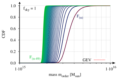
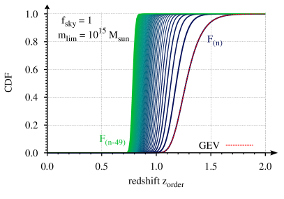
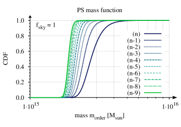
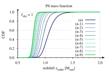
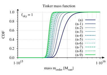
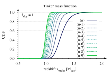
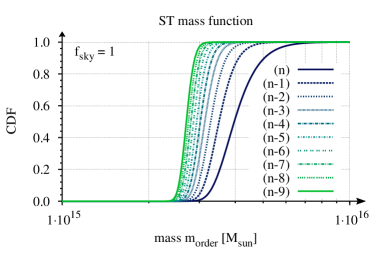
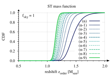
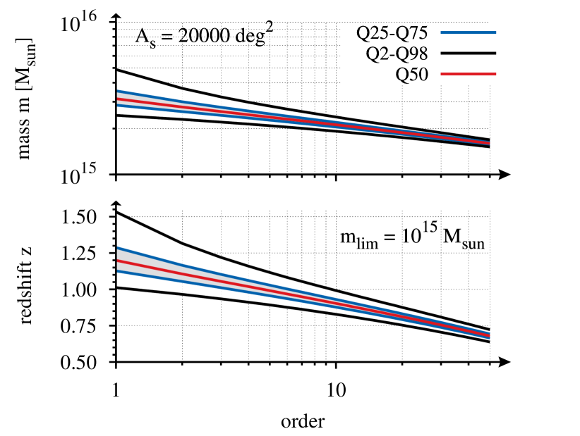
We calculated the distributions of the first fifty orders from $F_{(n)}(x)$ to $F_{(n-49)}(x)$, where $n=N_{\rm tot}$, and present the results in Fig. 1 for the mass (left panel) and redshift (right panel). In both panels the color decodes the order of the distribution, ranging from the blue for $F_{(n)}(x)$ to the green for $F_{(n-49)}(x)$. For both cases we assumed $f_{\rm sky}=1$, a redshift range of $0\leq z\leq\infty$ and the Tinker et al. (2008) mass function. In the case of the order statistics in redshift, we assume a limiting survey mass of $m_{\rm lim}=10^{15}\,M_{\odot}$. It can be nicely seen how, with increasing order (from blue to green), the cdfs shift in both cases to smaller values of the mass or redshift.

A first important result is that, with the increasing order, the cdfs steepen, which results in an enhanced constraining power, since small shifts in the mass or redshift may yield large differences in the derived probabilities. In this sense the higher orders will be more useful for falsification experiments than the extreme value distribution which, due to its shallow shape, requires extremely large values of the observable to statistically rule out the underlying assumptions. Since higher orders encode information from the $n$ most extreme objects, deviations from the expectation are statistically more significant for $n$ values instead of a single extreme one.

In addition, we compare the distribution of the maxima $F_{(n)}(m)$ and $F_{(n)}(z)$ to those obtained from a extreme value approach (Davis et al., 2011; Waizmann et al., 2012a, Metcalf & Waizmann in prep.) based on the void probability (White, 1979), using equation 5. For both cases presented in Fig. 1, the red, dashed curve of the GEV distribution, $G(x)$, agrees very well with the directly calculated $F_{(n)}(x)$.

In order to allow a quick estimation of the distributions of the order statistics, we provide in the Appendix B also fitting formulae for $F(x)$ as a function of the survey area for the cases of mass and redshift. The fitting formulae for the distribution in mass allow an estimation of the quantiles in the range from the 2-percentile, $Q2$, to the 98-percentiles, $Q98$, with an accuracy better than one per cent for $A_{\rm s}\gtrsim 200\,{\rm deg}^{2}$ and for the ten largest masses. In the instance of the order statistics in redshift, the quality of the fits depends on $m_{\rm lim}$ as well. For $m_{\rm lim}=10^{15}\;M_{\odot}$ an accuracy of better than two per cent can be achieved for $A_{\rm s}\gtrsim 2000\,{\rm deg}^{2}$ and for $m_{\rm lim}=5\times 10^{14}\;M_{\odot}$ the same accuracy is obtained down to $A_{\rm s}=100\,{\rm deg}^{2}$. A more detailed discussion of the fitting functions and their performance can be found in Appendix B.

In the remaining part of this work, we will discuss how the underlying cosmological model affects the order statistics and confront the theoretically derived order statistics with observations, afterwards.

Figure 2: Relative differences in the 98 percentile, $Q98$, with respect to the $\Lambda$CDM case for the order statistics in mass (blue lines), in mass with a lower redshift limit of $z=1$ (green lines) and in redshift (red lines) as a function of different cosmological parameters. The upper left panel shows the variation with $\sigma_{8}$, the upper right panel the one with $\Omega_{\rm m}$, the lower left one the one with the constant equation of state parameter $w_{0}$ and the lower right one shows the variation with the derivative of a linearised model for a time dependent equation of state $w_{a}$. The different line-styles denote different orders as indicated in the individual panels. For all calculations, the full sky and the Tinker mass function were assumed.

Figure 3: Impact of the different mass function on the cdfs of the first ten orders $F_{(n)},\dots,F_{(n-9)}$ in mass (left column) and redshift (right column). All distributions were computed for the full sky and three different mass functions comprising the Press-Schechter (PS), the Tinker and the Sheth& Tormen (ST) ones, ordered from top to bottom. For the distributions in redshift, a limiting survey mass of $m_{\rm lim}=10^{15}\,M_{\odot}$ has been assumed.

3 Dependence of the order statistics on the underlying cosmology

Eventually, the order statistics in mass and redshift is determined by the number of galaxy clusters in a given cosmic volume. The quantities that impact on this number can be categorised into two classes. The first one contains all effects that modify structure formation itself, like the choice of the mass function or the amplitude of the mass fluctuations, $\sigma_{8}$, for instance. These effects manifest themselves most strongly in the exponentially suppressed tail of the mass function, hence at high masses. The second class contains all the effects that modify the geometric evolution of the Universe. By changing the evolution of the cosmic volume, the number of clusters in a given redshift range can be substantially different, even if both cosmologies yield the same the number density of objects of a given mass (see e.g. Pace et al., 2010).

3.1 Impact of cosmological parameters

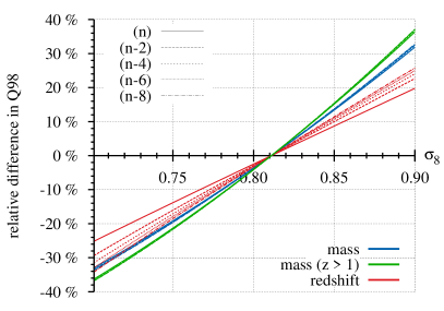
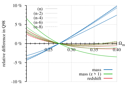
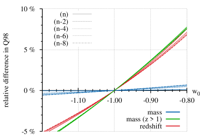
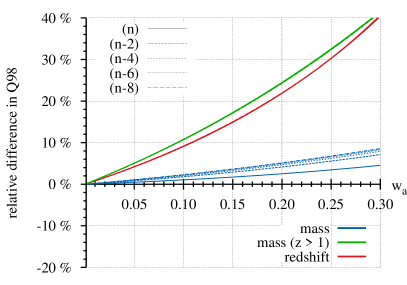
In order to quantify the impact of different cosmological parameters on the order statistics in mass and redshift, we study the effect on the $98$-percentile, $Q98$, which we use to define possible outliers from the underlying distribution. In Fig. 2, we present the relative difference in $Q98$ as a function of four different cosmological parameters comprising $\sigma_{8}$, $\Omega_{\rm m}$ (assuming the flatness constraint), the equation of state parameter, $w_{0}$, and the derivative $w_{a}$ from the relation $w(a)=w_{0}+w_{a}(1-a)$, where $a$ denotes the scale factor. A non-vanishing value of the latter indicates a time-varying equation of state. In each panel of Fig. 2, we show the relative differences for $5$ different orders, of the order statistic in mass with $z\in[0,\infty]$ (blue lines) and $z\in[1,\infty]$ (green lines), as well as in redshift (red lines) assuming $m_{\rm lim}=10^{15}\,M_{\odot}$. For all calculations we assumed the full sky and the Tinker et al. (2008) mass function.

It can be seen that order statistics is very sensitive to $\sigma_{8}$, such that the relative differences in $Q98$ would amount to $\sim 7$ per cent for the range allowed by WMAP7 of $(\sigma_{8}=0.811\pm 0.023)$. All three order statistics exhibit the same functional behaviour, with the mass-based ones being more sensitive than the redshift-based one. This can be understood by the fact that the mass-based order statistics probe the most massive clusters and hence the exponential tail of the mass function which is highly sensitive to $\sigma_{8}$.

For modifications of the matter density, $\Omega_{\rm m}$, assuming the flatness constraint $\Omega_{\Lambda}=1-\Omega_{\rm m}$, the situation is substantially different from the previous case (see upper right panel of Fig. 2). Overall, the order statistics are less sensitive and they do not exhibit the same functional behaviour. The order statistics in mass (blue lines) performs best for larger value of $\Omega_{\rm m}$ because the most massive clusters will reside at rather low redshifts. At high redshifts (green and red lines), the increase in $\Omega_{\rm m}$ and hence, the decrease in $\Omega_{\Lambda}$, yields a smaller number of very massive clusters. Despite the increase in the matter density, the decrease in volume is dominating for the range of $\Omega_{\rm m}$ shown in the plot and, thus, the relative difference decreases. In this sense the volume effects dominate at high redshifts over the increase in matter density, whereas at low redshifts the increase in matter density dominates.

The lower left panel of Fig. 2 shows the sensitivity of the order statistics to changes in the constant equation of state, $w_{0}$. Evidently, the most massive clusters at low redshifts (blue line) have no sensitivity to $w_{0}$, whereas at high redshifts (green and red line) the sensitivity is better. The volume effects are, compared to modifications in $\Omega_{\rm m}$, less important and the observed increase in the relative difference in $Q98$ with decreasing $w_{0}$ is dominated by modifications of the exponential tail of the mass function (for a more thorough discussion, see e.g. Pace et al., 2010).

When assuming a time-dependent equation of state, modelled by $w(a)=w_{0}+w_{a}(1-a)$, as presented in the lower right panel of Fig. 2, the observed functional behaviour can be explained by identical arguments as before. The results exhibit again the high sensitivity of the high redshift order statistics on modifications of $w_{a}$. It should be noted that we fixed $w_{0}=-1.0$ for all cases.

It can be summarised that for modifications that strongly affect the structure formation, like $\sigma_{8}$ for instance, the order statistics in mass for $z\in[0,\infty[$ is comparable in its sensitivity to the redshift based order statistics. Modifications that strongly alter the geometric evolution of the Universe affect more strongly the order statistics in redshift. However, one should keep in mind that in the case of the order statistics in mass, the relative differences are on the same level as the inaccuracies in cluster mass estimates. This problem does not occur for redshifts, which can be measured to a very high accuracy. Of course, in this case the observational challenge is transferred to compiling a sample with a precise mass limit. Apart from the cosmological parameters also the choice of the mass function is expected to have a strong effect on the order statistics as will be discussed in the following subsection.

Table 1: Compilation of the ten most massive galaxy clusters from the SPT massive cluster sample (Williamson et al., 2011) and the MCXC catalogue (Piffaretti et al., 2011), respectively. The masses $M_{200\rm m}$ and $M_{200\rm m}^{\rm Edd}$ are with respect to the mean background density before and after the correction for the Eddington bias based on the estimated mass uncertainty $\sigma_{\ln M}$. The last column lists the references for the values of the observed mass, on which the analysis is based on.

Rank	Cluster	$z$	$M_{200\rm m}$ in units of $M_{\odot}$	$\sigma_{\ln M}$	$M_{200\rm m}^{\rm Edd}$ in units of $M_{\odot}$	Reference
SPT catalogue $\mathbf{(A_{\rm s}=2500\,{\rm deg}^{2})}$
$1^{\rm st}$	SPT-CL J0658-5556	0.296	$(3.12\pm 1.15)\times 10^{15}$	0.39	$1.99_{-0.64}^{+0.95}\times 10^{15}$	Williamson et al. (2011)
$2^{\rm nd}$	SPT-CL J2248-4431	0.348	$(2.90\pm 1.03)\times 10^{15}$	0.37	$1.91_{-0.59}^{+0.86}\times 10^{15}$	”
$3^{\rm rd}$	SPT-CL J0102-4915	0.870	$(2.16\pm 0.32)\times 10^{15}$	0.15	$1.98_{-0.28}^{+0.32}\times 10^{15}$	Menanteau et al. (2012)
$4^{\rm th}$	SPT-CL J0549-6204	0.320	$(1.99\pm 0.67)\times 10^{15}$	0.35	$1.48_{-0.44}^{+0.62}\times 10^{15}$	Williamson et al. (2011)
$5^{\rm th}$	SPT-CL J0638-5358	0.222	$(1.91\pm 0.62)\times 10^{15}$	0.34	$1.50_{-0.44}^{+0.61}\times 10^{15}$	”
$6^{\rm th}$	SPT-CL J0232-4421	0.284	$(1.88\pm 0.59)\times 10^{15}$	0.32	$1.48_{-0.41}^{+0.56}\times 10^{15}$	”
$7^{\rm th}$	SPT-CL J0645-5413	0.167	$(1.81\pm 0.60)\times 10^{15}$	0.34	$1.43_{-0.41}^{+0.58}\times 10^{15}$	”
$8^{\rm th}$	SPT-CL J0245-5302	0.098	$(1.70\pm 0.46)\times 10^{15}$	0.25	$1.48_{-0.33}^{+0.42}\times 10^{15}$	”
$9^{\rm th}$	SPT-CL J2201-5956	0.300	$(1.70\pm 0.42)\times 10^{15}$	0.28	$1.48_{-0.36}^{+0.48}\times 10^{15}$	”
$10^{\rm th}$	SPT-CL J2344-4243	0.450	$(1.65\pm 0.38)\times 10^{15}$	0.31	$1.28_{-0.34}^{+0.47}\times 10^{15}$	”
MCXC catalogue $\mathbf{(A_{\rm s}=27490\,{\rm deg}^{2})}$
$1^{\rm st}$	J0417.5-1154	0.4430	$(3.86\pm 0.62)\times 10^{15}$	0.15	$3.55_{-0.49}^{+0.57}\times 10^{15}$	Piffaretti et al. (2011)
$2^{\rm nd}$	J2211.7-0349	0.3970	$(3.21\pm 0.51)\times 10^{15}$	0.15	$2.98_{-0.42}^{+0.48}\times 10^{15}$	”
$3^{\rm rd}$	J2243.3-0935	0.4470	$(3.04\pm 0.49)\times 10^{15}$	0.15	$2.82_{-0.39}^{+0.46}\times 10^{15}$	”
$4^{\rm th}$	J0308.9+2645	0.3560	$(2.95\pm 0.47)\times 10^{15}$	0.15	$2.75_{-0.38}^{+0.45}\times 10^{15}$	”
$5^{\rm th}$	J1504.1-0248	0.2153	$(2.36\pm 0.35)\times 10^{15}$	0.14	$2.25_{-0.29}^{+0.34}\times 10^{15}$	”
$6^{\rm th}$	J1347.5-1144	0.4516	$(2.30\pm 0.41)\times 10^{15}$	0.16	$2.14_{-0.32}^{+0.37}\times 10^{15}$	”
$7^{\rm th}$	J1731.6+2251	0.3890	$(2.28\pm 0.37)\times 10^{15}$	0.15	$2.14_{-0.30}^{+0.35}\times 10^{15}$	”
$8^{\rm th}$	J0717.5+3745	0.5460	$(2.21\pm 0.35)\times 10^{15}$	0.15	$2.06_{-0.29}^{+0.33}\times 10^{15}$	”
$9^{\rm th}$	J2248.7-4431	0.3475	$(2.13\pm 0.35)\times 10^{15}$	0.15	$2.01_{-0.28}^{+0.33}\times 10^{15}$	”
$10^{\rm th}$	J1615.7-0608	0.2030	$(2.14\pm 0.30)\times 10^{15}$	0.13	$2.03_{-0.25}^{+0.28}\times 10^{15}$	”

3.2 Impact of the choice of the mass function

When performing a falsification experiment of $\Lambda$CDM using the $n$ most massive or $n$ highest redshift clusters, then one has to specify the reference model against which the observations have to be compared with. Apart from the cosmological parameters that are usually fixed to the obvious choice of the WMAP7 values, a halo mass function has to be chosen as well. As mentioned earlier, this is particularly important for galaxy clusters since the exponentially suppressed tail of the mass function is naturally very sensitive to modifications.

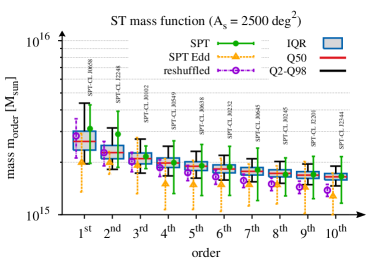
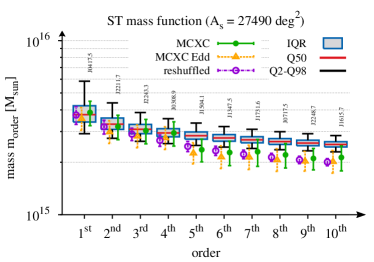
In order to quantify the impact of different mass functions on the order statistics in mass and redshift, we computed the cdfs, $F_{(n-9)},\dots,F_{(n)}$, for the Press & Schechter (1974) (PS), the Tinker et al. (2008) and the Sheth & Tormen (1999) (ST) mass functions for $f_{\rm sky}=1$ and present them from top to bottom in Fig. 3. Comparing the panels to each other reveals the tremendous sensitivity of the distributions to the choice of the mass function. Taking the Tinker mass function as a reference, the median, $Q50$, changes for both types of order statistics by $-20$ per cent for the PS case and by $+15$ percent for the ST case. These differences can be explained by the fact that the ST mass function leads to a substantial increase in the number of haloes, particularly at the high mass end, whereas the PS mass function results in much fewer haloes in the mass and redshift range of interest. For the remainder of this paper we will use the Tinker mass function as reference because the halo masses are defined as spherical overdensities with respect to the mean background density, a definition that is closer to theory and actual observations than friend-of-friend masses.

However, considering that due to statistical limitations, current fits for the mass function are still not very accurate for the highest masses $(>3\times 10^{15}\,M_{\odot})$ and that systematic uncertainties allow even smaller masses an accuracy of a few per cent at most (Bhattacharya et al., 2011), one has to be very cautious with falsification experiments that are based on extreme objects. The uncertainty in the mass function alone will allow a rather wide range of distributions.

4 Suitable samples of galaxy clusters for an order statistical analysis

Having introduced the order statistics of the most massive or the highest redshift clusters, we intend now to compare observed clusters with the theoretical distributions. To do so, it is necessary to select suitable samples of galaxy clusters, which we will discuss in the following.

4.1 General considerations

The selection of a suitable sample of galaxy clusters for an order statistical analysis is by no means a trivial task. The necessary ordering of the quantities mass and redshift by magnitude requires that they have been derived in an identical way across the sample. Otherwise, systematics and biases, like the differences between lensing and X-ray mass estimates for instance (see e.g. Mahdavi et al., 2008; Zhang et al., 2010; Planck Collaboration et al., 2012; Meneghetti et al., 2010; Rasia et al., 2012), will render the ordering meaningless. Despite an increasing amount of data from different surveys, a lack of large homogeneous samples persists. Thus, we decided to base our comparison on clusters that stem from catalogues like the SPT massive cluster sample (Williamson et al., 2011) and the MCXC cluster catalogue (Piffaretti et al., 2011), which will be discussed in further detail below.

4.2 The SPT massive cluster sample

The SPT survey (Carlstrom et al., 2011) is ideally suited for the intended purpose of an order statistical analysis. Being based on the Sunyaev Zeldovich (SZ) effect (Sunyaev & Zeldovich, 1972, 1980) the SPT survey is able to detect massive galaxy clusters up to high redshifts. The fact that the limiting mass of SZ surveys varies weakly with redshift (Carlstrom et al., 2002) allows in principle to construct mass limited cluster catalogues. However, it should be emphasised that the assumption of an $m_{\rm lim}$ independent of redshift depends critically on the sensitivity and the beam width of an actual survey.

For this work, we take the catalogue of Williamson et al. (2011) which comprises the 26 most significant detections in the full survey area of $A_{\rm s}^{\rm SPT}=2500\,{\rm deg}^{2}$. Ensuring a constant mass limit of $M_{200\rm m}\approx 10^{15}\,M_{\odot}$, clusters were selected on the basis of a signal-to-noise (S/N) threshold in the filtered SPT maps. For all 26 catalogue members, either photometric or spectroscopic redshifts were determined as well. The cluster masses given in the catalogue are defined with respect to the mean cosmic background density and need no further conversion to match the mass definition of the reference Tinker et al. (2008) mass function. To each cluster of the sample we assign the error bars that we obtained by adding the reported statistical and systematic errors in quadrature.

4.3 The MCXC cluster catalogue

The MCXC catalogue (Piffaretti et al., 2011) is based on the publicly available compilation of clusters’ detections from ROSAT All-Sky Survey (NORAS, REFLEX, BCS, SGP, NEP, MACS, and CIZA) and other serendipitous surveys (160SD, 400SD, SHARC, WARPS, and EMSS), and provides the physical properties of 1743 galaxy clusters systematically homogenised to an overdensity of 500 (with respect to the cosmic critical density). This meta-catalogue is not complete in any sense, but it is constituted by X-ray flux-limited samples that ensure that the X-ray brightest objects in the nearby ($z\la 0.3$) Universe, and therefore the most massive X-ray detected clusters, are all included.

We have then simply ranked the objects accordingly to their estimated $M_{200\rm m}$, that is obtained from the tabulated $M_{500\rm c}$ as

$$M_{200\rm m}=M_{500\rm c}\frac{200\Omega_{z}}{500}\left(\frac{R_{200\rm m}}{R_{500{\rm c}}}\right)^{3}$$ (13)

where $\Omega_{z}=\Omega_{\rm m}(1+z)^{3}/E_{z}^{2}$, $E_{z}=(\Omega_{\rm m}(1+z)^{3}+\Omega_{\Lambda})^{1/2}$, and the ratio between the radii at different overdensities has been obtained by assuming an NFW profile (Navarro et al., 1996) with $c_{200}=4$.

4.4 Preparations of the ordered samples

We order the SPT and MCXC catalogues by magnitude of the observed mass and present the ten most massive systems in Table 1. For statistical comparisons the observed masses have to be corrected for the Eddington bias (Eddington, 1913) in mass. As a result of the exponentially suppressed tail of the mass function and the substantial uncertainties in the mass determination of galaxy clusters, it is more likely that lower mass systems scatter up while higher mass systems scatter down, resulting in a systematic shift. Thus, before an observed mass can be compared to a theoretical distribution, this shift has to be corrected for. To do so, we follow Mortonson et al. (2011) and shift the observed masses, $M_{\rm obs}$, to the corrected masses, $M_{\rm corr}$, according to

$$\ln M_{\rm corr}=\ln M_{\rm obs}+\frac{1}{2}\epsilon\sigma_{\ln M}^{2},$$ (14)

where $\epsilon$ is the local slope of the mass function ($\mathrm{d}n/\mathrm{d}\ln M\propto M^{\epsilon}$) and $\sigma_{\ln M}$ is the uncertainty in the mass measurement. We corrected the observed masses in both, the SPT and the MCXC catalogues, using the values of $\sigma_{\ln M}$ listed in the fifth column of Table 1 which we deduced from the reported uncertainties in the nominal masses. The larger the observational errors are, the larger is the correction towards lower masses.

As an exemplary exception from the SPT catalogue, we used for the mass of SPT-CL J0102-4915 the value reported by Menanteau et al. (2012), which is based on a combined SZ+X-rays+optical+infrared analysis. The multi-wavelength study shifts $M_{\rm obs}=(1.89\pm 0.45)\times 10^{15}\,M_{\odot}$ (Williamson et al., 2011) to a larger value of $M_{\rm obs}=(2.16\pm 0.32)\times 10^{15}\,M_{\odot}$, changing the rank from the fifth to the third most massive. This shows that with the expected increase in the quality of cluster mass estimates, the ordering of the most massive cluster will undergo significant changes. We expect that the reshuffling will affect more strongly the most massive clusters due to the fact that the large error bars will cause lower ranked clusters to scatter up. We will discuss the impact of the reshuffling in more detail in Sect. 5.1.

In addition, we sorted the SPT catalogue by redshift and list the ten highest redshift clusters above $m_{\rm lim}\approx 10^{15}\,M_{\odot}$ in Table 2.

Table 2: Compilation of the ten highest redshift clusters from the SPT massive cluster sample (Williamson et al., 2011). Here, (s) and (p) denote the spectroscopic and photometric redshifts, respectively.

Rank	Cluster	$z$	$M_{200\rm m}$ in units of $M_{\odot}$
$1^{\rm st}$	SPT-CL J2106-5844	1.132 (s)	$(1.27\pm 0.21)\times 10^{15}$
$2^{\rm nd}$	SPT-CL J0615-5746	0.972 (s)	$(1.32\pm 0.40)\times 10^{15}$
$3^{\rm rd}$	SPT-CL J0102-4915	0.870 (s)	$(2.16\pm 0.32)\times 10^{15}$
$4^{\rm th}$	SPT-CL J2337-5942	0.775 (s)	$(1.99\pm 0.20)\times 10^{15}$
$5^{\rm th}$	SPT-CL J2344-4243	0.620 (p)	$(1.91\pm 0.50)\times 10^{15}$
$6^{\rm th}$	SPT-CL J0417-4748	0.620 (p)	$(1.88\pm 0.20)\times 10^{15}$
$7^{\rm th}$	SPT-CL J0243-4833	0.530 (p)	$(1.81\pm 0.23)\times 10^{15}$
$8^{\rm th}$	SPT-CL J0304-4401	0.520 (p)	$(1.70\pm 0.33)\times 10^{15}$
$9^{\rm th}$	SPT-CLJ0438-5419	0.450 (p)	$(1.70\pm 0.38)\times 10^{15}$
$10^{\rm th}$	SPT-CLJ0254-5856	0.438 (s)	$(1.65\pm 0.25)\times 10^{15}$

Figure 4: Functional box plots for the first nine orders in the observable mass as indicated in the individual panels. Here, the red line denotes the median ($Q$50), the blue-bordered, grey region the interquartile range (IQR) and the black lines denote the 2 and the 98-percentile ($Q$2, $Q$98). The green error bars show the corresponding observed masses, $M_{200\rm m}$, from the SPT (green circles) and the MCXC (green triangles) catalogues (see Table 1) for their respective survey areas of $A^{\rm SPT}_{\rm s}=2500\,{\rm deg^{2}}$ and $A^{\rm MCXC}_{\rm s}=27490\,{\rm deg^{2}}$.

Figure 5: Box-and-whisker diagram of the ten most massive clusters from the SPT survey (left column) and the MCXC catalogue (right column) for three different choices of the mass function as denoted in the title of each panel. For each order, the red lines denote the median ($Q$50), the blue-bordered, grey boxes give the IQR and the black whiskers mark the range between the $2$ and $98-$percentile ($Q$2, $Q$98) of the theoretical distribution. The green, filled circles denote the nominal observed cluster masses, $M_{200\rm m}$, the orange, empty triangles the ones that are corrected for the Eddington bias in mass and the violet, empty circles are the results of the Monte Carlo reshuffling of the ranks. All error bars denote the $1\sigma$ range.

Figure 6: Dependence of different percentiles on the order for the order statistics in mass (upper panel) and redshift (lower panel). For both cases a survey area of $A_{\rm s}=20\,000\,{\rm deg}^{2}$ is assumed. Further, a limiting mass of $m_{\rm lim}=10^{15}\,M_{\odot}$ has been adopted for the order statistics in redshift. All percentiles are denoted by the same line styles as used in the previous figures and are given in the key.

5 Comparison of the individual order statistics with observations

In this section we will compare the individual ranked systems listed in Table 1 for the mass and in Table 2 for the redshift with the individual distributions for each rank, as e.g. shown in Fig. 3.

5.1 Order statistics in cluster mass

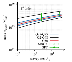
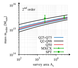
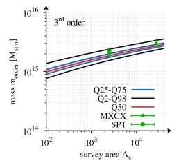
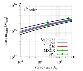
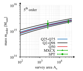
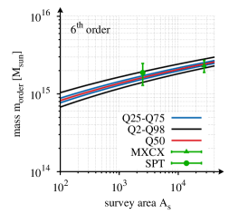
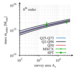
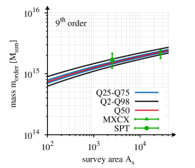
In order to demonstrate the impact of the survey area on the distributions of the order statistics in mass, we show in Fig. 4 the dependence of different quantiles ($Q$2, $Q$25, $Q$50, $Q$75 and $Q$98) on the survey area for the nine most massive clusters. In addition, the green error bars show the clusters from the SPT and MCXC catalogues listed in Table 1 for the respective survey areas of $A^{\rm SPT}_{\rm s}=2500\,{\rm deg^{2}}$ and $A^{\rm MCXC}_{\rm s}=27490\,{\rm deg^{2}}$.

From the individual panels in Fig. 4 it can be inferred that, as expected, a larger survey area yields a larger expected mass for the individual rank. Furthermore, with increasing rank towards higher orders, the interquantile range, like (Q2-Q98), narrows. A behaviour that can also be seen in Fig. 1 as steepening of the cdf with increasing rank. Therefore, the largest mass (first order) is expected to be realised in a much wider mass range than the higher orders.

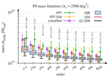
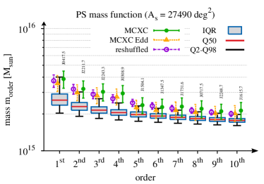
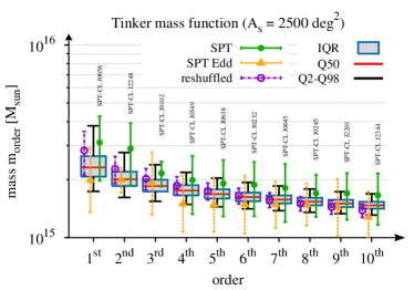
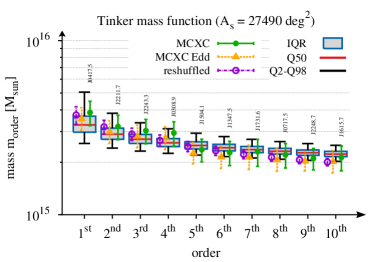
We will now compare the observations in more detail with the theoretical expectations in the form of box-and-whisker diagrams as shown in Fig. 5. Here, the blue-bordered, grey filled box denotes the interquartile range (IQR) which is bounded by the 25 and 75-percentiles ($Q$25, $Q$75) and the median ($Q$50) is depicted as a red line. The black whiskers denote the 2 and 98-percentiles ($Q$2,$Q$98) and we follow the convention that observations that fall outside are considered as outliers. As before, the nominal observed cluster masses are denoted as green error bars where for the left column the SPT catalogue and for the right column the MCXC catalogue was used. In addition we plot the Eddington bias corrected masses, $M_{200\rm m}^{\rm Edd}$, from the sixth column of Table 1 as orange triangles with dashed error bars. We performed the analysis for three different mass functions, comprising from the top to the bottom panel, the PS, the Tinker and the ST mass functions. In addition to the Eddington bias in mass, we expect a shift to larger masses caused by the reshuffling of orders due to the uncertainties in mass. In order to quantify this effect, we Monte Carlo (MC) simulated $10\,000$ realisations of the 26 SPT and 123 MCXC (with $M>10^{15}\,M_{\odot}$) cluster masses after their correction for the Eddington bias and order them by mass. The masses were randomly drawn from the individual error interval, assuming Gaussian distributions. We present the results as violet, empty circles with dash-dotted $1\sigma$ error bars in Fig. 5. It can be seen that the highest ranks are more strongly affected by the reshuffling than the lower ones and that they are on average shifted to larger values. Of course, the amount of this effect will depend on the size of the error bars. Further, the reshuffling yields mass values that fall between the nominal (green error bars) and the Eddington bias corrected ones (orange error bars).

For the SPT catalogue, it can be seen from the top left panel of Fig. 5 that the outdated PS mass function seems to be disfavoured by the reshuffled and the nominal masses of the ten largest objects. However, the error bars are large and do not allow an exclusion of the PS mass function. For the Tinker and the ST mass function, the boxes indicating the theoretical distributions move to larger mass values and therefore they match the observed masses better than the PS mass function. In particular, the third ranked (second ranked after Eddington bias correction) system SPT-CL J0102 with its smaller errors and, hence, giving the tightest constraints, is consistent with $\Lambda$CDM for both mass functions. All other ranks are consistent as well due to their large error bars. The reshuffled sample matches perfectly the Tinker mass function consolidating the conclusion that the most massive clusters of the SPT sample are in agreement with the statistical expectations. The conclusions for the MCXC catalogue are identical, however the jump between the fourth and the fifth largest order yield to an inconsistency of the observed higher orders with the expectations based on the ST mass function. This jump is clearly caused by the incompleteness of the MCXC catalogue and, thus, the inclusion of the missing clusters would most certainly move the observed sample to higher masses in the direction of the results we obtained from the SPT sample. In this sense we do not see any indication of a substantial difference between the small and wide field survey.

The analysis of the SPT sample illustrates the potential of utilising the $n$ most massive galaxy clusters to test underlying assumptions, like e.g. the mass function. For instance, a multi-wavelength study of the 26 SPT clusters would reduce the error bars to the level of SPT-CL J0102 (the nominal third ranked cluster in the left column of Fig. 5 ), which would significantly tighten the constraints on the underlying assumptions like e.g. the halo mass function. In turn, by assuming the $\Lambda$CDM reference cosmology, the comparison of the observed masses with the individual order distributions allows to check the completeness of the observed sample.

In the upper panel of Fig. 6, we present the dependence of different percentiles ($Q2$,$Q25$,$Q50$,$Q75$ and $Q98$) on the order for a survey area of $A_{\rm s}=20\,000\,{\rm deg}^{2}$. Choosing the $Q98$ percentile as exclusion criterion, one would need roughly to find ten clusters with $m\gtrsim 2.5\times 10^{15}\,M_{\odot}$, three clusters with $m\gtrsim 3.2\times 10^{15}\,M_{\odot}$ or one cluster with $m\gtrsim 5\times 10^{15}\,M_{\odot}$ in order to report a significant deviation from the $\Lambda$CDM expectations. Of course, the observed masses might have to be corrected for the Eddington bias in mass and a possible reshuffling as previously demonstrated. In general, exclusion criteria based on order statistics extend previous works (Mortonson et al., 2011; Waizmann et al., 2012a) from statements about single objects to statements about object samples which considerably improves the reliability of the entire study.

Figure 7: Functional box plot for the first nine orders in the observable redshift as indicated in the individual panels. Here, the red line denotes the median ($Q$50), the blue-bordered, grey region the interquartile range (IQR) and the black lines denote the 2 and the 98-percentile ($Q$2, $Q$98). The green circles (with error bars in the case of photometric redshifts) denote the redshifts from the SPT catalogue as listed in Table 2.

5.2 Order statistics in cluster redshift

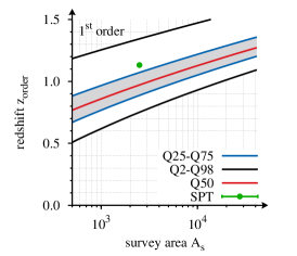
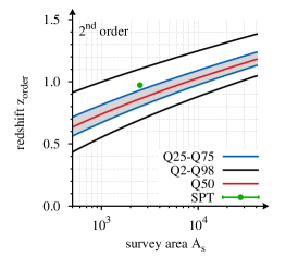
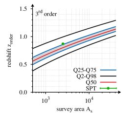
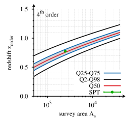
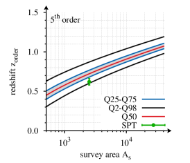
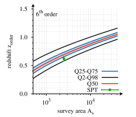
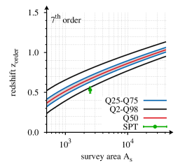
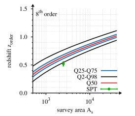
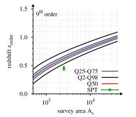
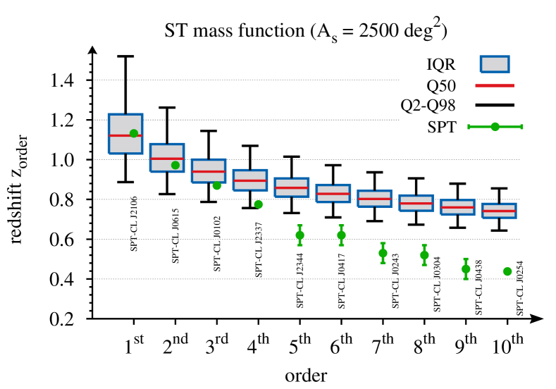
We performed an identical analysis for the individual order statistics for the SPT massive cluster catalogue ranked by redshift listed in Table 2. For the theoretical distributions we assume a limiting mass of $m_{\rm lim}=10^{15}\,M_{\odot}$ and a survey area of $A^{\rm SPT}_{\rm s}=2500\,{\rm deg^{2}}$. As before, we present in Fig. 7 the dependence of the order statistical distributions on the survey area for the first nine orders. Again, an increase in the survey area yields a shift of the theoretical distributions to higher redshifts and, as shown in the right panel of Fig. 1, the cdfs steepen for the higher ranks, resulting in a shrinking interquantile range.

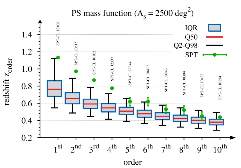
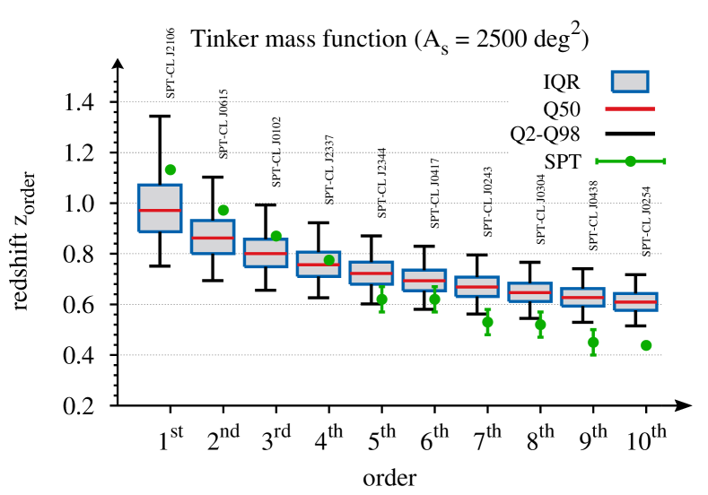
In Fig. 8, we present the box-and-whisker diagram in redshift, again for the PS, the Tinker and the ST mass functions (from top to bottom). The definition of boxes and whiskers remains unchanged with respect to Fig. 5. Again, the data from Table 2 is denoted by green error bars, which are negligibly small in the case of spectroscopic redshifts. Thus, we abstained from the MC simulation of the reshuffling in the case of redshift. While for the order statistics in mass the results only depended on the choice of the survey area, the situation is different for the order statistics in redshift. Here, a constant survey limiting mass is assumed, which will be subject to uncertainties for a real survey and, furthermore, will also exhibit some redshift dependence. Thus, the theoretical distributions are intrinsically less accurate than the ones with respect to cluster mass. Indeed, the comparison with the data in Fig. 8 exhibits a different behaviour with respect to the one in Fig. 5. Here, first four orders seem to be fit better by the Tinker mass function while the higher orders seem to favour the PS mass function. Taking the Tinker mass function as reference it seems that a few systems with $M>10^{15}\,M_{\odot}$ are missing at redshifts $z\gtrsim 0.7$. The difference with respect to the findings for the order statistics in mass for the same sample could, along the lines of Sect. 3, be interpreted as a signature of a deviation from the reference $\Lambda$CDM model. However, considering the previously mentioned simplifying assumptions in the modelling of the theoretical distributions, we do not infer any cosmological conclusions and leave a better, more realistic, modelling of $m_{\rm lim}(z)$ of the SPT survey to a future work.

In the lower panel of Fig. 6, we present the dependence of different percentiles ($Q2$,$Q25$,$Q50$,$Q75$ and $Q98$) on the order for a survey area of $A_{\rm s}=20\,000\,{\rm deg}^{2}$ and a constant limiting mass of $m_{\rm lim}=10^{15}\,M_{\odot}$. Taking the $Q98$ percentile as exclusion criterion, one would need to find ten clusters with $z\gtrsim 1$, three clusters with $z\gtrsim 1.2$ or one cluster with $z\gtrsim 1.55$ in order to report a significant deviation from the $\Lambda$CDM expectations. Currently, SPT-CL J2106 is the only known cluster of such a high mass having a redshift $z>1$. With an assigned survey area of $A_{s}=2800\,{\rm deg}^{2}$ (ACT+SPT), it might from a statistical point of view still be possible to find ten objects that massive at $z>1$ in the larger survey area. The method presented in this work allows to construct similar exclusion criteria for any kind of survey design.

Figure 8: Box-and-whisker diagram of the ten highest redshift clusters from the SPT catalogue as listed in Table 2 for three different choices of the mass function as denoted in the title of each panel. For each order, the red lines denote the median ($Q$50), the blue-bordered, grey boxes give the IQR and the black whiskers mark the range between the $2$ and $98-$percentile ($Q$2, $Q$98). The green circles (with error bars in the case of photometric redshifts) represent the observed cluster redshifts.

6 Comparison of the joint order statistics with observations

Having studied the individual order statistics in mass and redshift in the previous section, we turn now to the study of the joint distributions of the order statistics as introduced in Sect. 2.1.

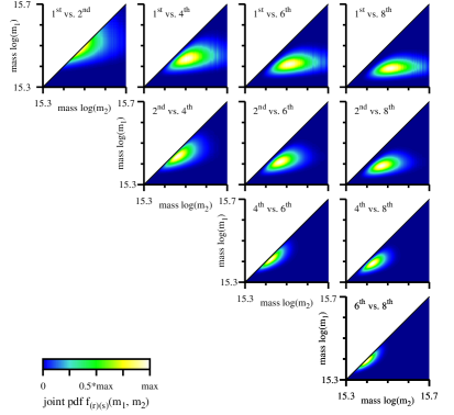
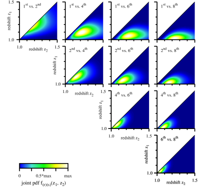
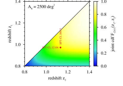
The simplest case of a joint order distribution is two-dimensional. In this case the pdf and cdf are given by equation 6 and equation 7, respectively. Starting with the joint pdf, we present in Fig. 9 the joint distributions in mass (left panel) and redshift (right panel) for several order combinations as denoted in the individual panels. All calculations assume the full sky and the Tinker mass function. In the case of the joint distributions in redshift, we assume a constant limiting survey mass of $m_{\rm lim}=10^{15}\,M_{\odot}$. Due to the condition that $x<y$, all distributions are limited to a triangular domain.

An inspection of the different pdfs in Fig. 9 reveals that, for the combination of the first and the second largest order (upper leftmost panel), the most likely combination of the observables is very close to the diagonal. This means that it is more likely to find the two largest values close to each other, at absolute values that are smaller than the extreme value statistics would imply for the maximum alone. Then, when moving to combinations of the first with higher orders (first row), it can be seen that the peaks of the pdfs move away from the diagonal and that they extend to larger values for the larger observable. This indicates that it is more likely to find the two systems with a larger separation in the observable when the difference between the considered orders is larger. Accordingly, for higher order combinations (lower rows), the peaks of the joint pdf move to smaller values of the observables. It should also be noted that the peaks steepen for higher order combinations, confining the pdfs to smaller and smaller regions in the observable plane. As an example, the first and second largest observations (upper leftmost panel) can be realised in much larger area than the sixth and eighth largest one (lower rightmost panel).

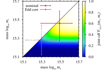
Apart from the joint pdfs, it is also instructive to study the joint cdfs as presented in Fig. 10 for the observed mass (left panel) and redshift (right panel). In order to add observational data from the SPT catalogue, we assume a survey area of $A_{\rm s}^{\rm SPT}=2500\,{\deg}^{2}$ and a $m_{\rm lim}=10^{15}\,M_{\odot}$ for the joint distribution in redshift. Additionally, we added the two largest nominal observed (red error bars) and the Eddington bias corrected masses (grey error bars) from Table 1 to the left panel and the two highest redshifts of the SPT massive cluster sample from Table 2 to the left panel. In the case of the mass, we find $F_{(n-1)(n)}\approx 0.92$ for the nominal and $F_{(n-1)(n)}\approx 0.1$ for the Eddington bias corrected masses. Hence, using the central values, in $\sim(8-90)$ percent of the cases a mass larger than the one of SPT-CL J0658 and a mass larger than the one of SPT-CL J2248 are observed. Thus, also the joint cdf confirms that the two largest masses do not exhibit any tension with the concordance cosmology. The same conclusion applies in the case of the joint distribution in redshift.

By means of equation 8 these results can be extended to the $n$-dimensional case, allowing the formulation of a likelihood function of the ordered sample of the $n$ most massive or highest redshift clusters.

Figure 9: Joint pdf $f_{(r)(s)}(x,y)$ (see equation 6) for the observable mass (left panel) and redshift (right panel) for different combinations of rank as indicated in the upper left of each small panel. The distributions are calculated for the fullsky and a constant limiting survey mass of $m_{\rm lim}=10^{15}\,M_{\odot}$ has been assumed for the joint distribution in redshift. The color bar is set to range from 0 to the maximum of the joint pdf for each rank combination.

Figure 10: Joint cdf $F_{(r)(s)}(x,y)$ (see equation 7) for the observable mass (left panel) and redshift (right panel) for the combination of the largest and second largest observation, assuming a survey area of $A_{\rm s}^{\rm SPT}=2500\,{\deg}^{2}$ and a constant limiting survey mass of $m_{\rm lim}=10^{15}\,M_{\odot}$ for the joint distribution in redshift. The red and grey error bars denote the nominal and the Eddington bias corrected values, $M_{200\rm m}$ and $M_{200\rm m}^{\rm Edd}$, for the SPT catalogue as listed in Table 1 for the mass and in Table 2 for the redshift.

7 Summary

In this work, we studied the application of order statistics to the mass and redshifts of galaxy clusters and compared the theoretically derived distributions with observed samples of galaxy clusters. Our work extends previous studies that hitherto considered only the extreme value distributions in mass or redshift.

On the theoretical side, our results can be summarised as follows.

1. We introduce all relations necessary to calculate pdfs and cdfs of the individual and joint order statistics in mass and redshift. In particular, we find a steepening of the cdfs for higher order distributions with respect to the extreme value distribution of both mass and redshift. This steepening corresponds to a higher constraining power from distributions of the $n$-largest observations. The presented method extends previous works to include exclusion criteria based on the $n$ most massive or $n$ highest redshift clusters for a given survey set-up.

2. Conceptually, we avoid the bias due to an a posteriori choice of the redshift interval in the case of the order statistics in mass by selecting the interval $0\leq z\leq\infty$. Hence, we study the statistics of the hierarchy of the most massive haloes in the Universe, which mostly stem from redshifts $z\lesssim 0.5$. On the contrary, when choosing the order statistics in redshift, focus is laid on haloes that stem from the highest possible redshifts. However, the calculations will require a model of the survey characteristics in the form of a limiting survey mass as a function of redshift.

3. By putting the emphasis on either the most massive or on the highest redshift clusters above a given mass limit, the order statistics is e.g. particularly sensitive to the choice of the mass function. While the order statistics in mass is very sensitive to $\sigma_{8}$ and $\Omega_{\rm m}$ due to the domination of low redshift objects, the order statistics in redshift proves to be very sensitive to $w_{0}$ and $w_{a}$. For a fixed cosmology, both order statistics are efficient probes of the functional shape of the mass function at the high mass end.

4. In addition to the individual order statistics, we study as example case also the joint two order statistics. We find that for the combination of the largest and the second largest observation, it is most likely to find them to be realised with very similar values with a relatively broadly peaked distribution.

5. In order to allow a quick estimation of the distributions of the order statistics, we provide in the Appendix B fitting formulae for $F(x)$ as a function of the survey area for the cases of mass and redshift. The fitting formulae for the distribution in mass allow for a percentile estimation in the range from $Q2$ to $Q98$ with an accuracy better than one per cent for $A_{\rm s}\gtrsim 200\,{\rm deg}^{2}$ and for the ten largest masses. In the case of the order statistics in redshift, the quality of the fits depends on the chosen $m_{\rm lim}$. However, for survey areas of $A_{\rm s}\gtrsim 2000\,{\rm deg}^{2}$ accuracies better than two per cent can be achieved for large values of $m_{\rm lim}=10^{15}\;M_{\odot}$ and a lowering of $m_{\rm lim}$ further improves the accuracy.

After introducing the theoretical framework, we compared the theoretical distributions with actually observed samples of galaxy clusters that we ranked by the magnitude of the observables mass and redshift. We decided to compile two catalogues, the main one is based on the SPT massive cluster sample (Williamson et al., 2011) and additionally we analysed the meta-catalogue of X-ray detected clusters of galaxies MCXC (Piffaretti et al., 2011) based on publicly available flux-limited all-sky survey and serendipitous cluster catalogues. This meta-catalogue can be considered as complete for $z\lesssim 0.3$ and, hence, by no means as complete as the SPT one. The results of the comparison can be summarised as follows.

1. In the case of the order statistics in mass, we compared the theoretical expectations for the ten largest masses for the PS, the Tinker and the ST mass functions. Assuming WMAP7 parameters, we find that the nominal and the Eddington bias corrected values for the observed masses favour the Tinker and the ST mass functions. When considering the possible bias due to a reshuffling of the ranks caused by the large error bars (statistical + systematic errors), we find that the SPT sample matches the Tinker mass function very well. The constraints are expected to tighten considerably once the error bars of all objects are scaled down by combining several cluster observables in multi-wavelength studies.

2. In contrast to the ranking in mass, the order statistics of the SPT clusters in redshift is less well fit by the theoretical distributions based on the Tinker mass function. It appears that a few systems with $M>10^{15}\,M_{\odot}$ are missing at redshifts $z\gtrsim 0.7$. One explanation could be found in a non-standard cosmological evolution to which the order statistics in redshift is more sensitive. However, it is more likely that a more precise modelling (including the redshift dependence) of the true limiting survey mass of SPT will account for the observed deviations.

3. Instead of utilising order statistics to perform exclusion experiments, it can also be used for consistency checks of the completeness of the observed sample and of the modelling of the survey selection function as indicated by the analysis of the MCXC (mass) and the SPT (redshift) samples.

8 Conclusions

We introduced a powerful theoretical framework which allows to calculate the expected individual and joint distribution functions of the $n$-largest masses or the $n$-highest redshifts of galaxy clusters in a given survey area. This approach is more powerful than the extreme value statistics that focusses on the statistics of the single largest observation alone.

As a proof of concept, we compared the theoretical distributions with observed samples of galaxy clusters. However, data of sufficient quantity, uniformity and completeness is still sparse such that constraints are not particularly tight. This situation will most certainly improve in the near and intermediate future. Since the emphasis of this work lies on the introduction of the theoretical framework of order statistics and its application to galaxy clusters, we contended ourselves with a study of cluster masses and redshifts. Unfortunately, the mass of a galaxy cluster is not a direct observable and subject to large scatter and observational biases. In a follow-up work, we intend to extend the formalism to direct observables, like for instance X-ray luminosities, and to include the scatter in the scaling relations into the theoretical distributions.

Appendix A Order statistics

In this appendix, we outline the derivation of the most important relations of the order statistics and some subtleties considering their implementation. For more details we refer to the excellent textbooks on the topic by Arnold et al. (1992) and by David & Nagaraja (2003) which we closely follow for the remainder of this appendix.

A.1 Individual distributions

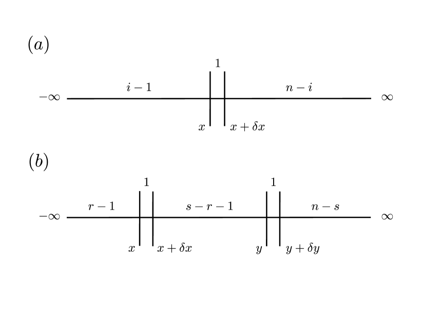
Let $X_{1},X_{2},\dots,X_{n}$ be a random sample of a continuous population with the cumulative distribution function, $F(x)$. Further, let $X_{(1)}\leq X_{(2)}\leq\cdots\leq X_{(n)}$ be the order statistic, the random variates ordered by magnitude, where $X_{(1)}$ is the smallest (minimum) and $X_{(n)}$ denotes the largest (maximum) variate. The event $x<X_{(i)}\leq x+\delta x$ is the same as the one depicted in panel $(a)$ of Fig. 11 and, thus, we have $X_{k}\leq x$ for $i-1$ of the $X_{k}$, exactly one $X_{k}$ in $x<X_{k}\leq x+\delta x$ and the remaining $n-i$ of the $X_{k}$ in $X_{k}>x+\delta x$. Now, the number of ways how $n$ observations can be arranged in the three regimes is given by

$$A(n,i)=\frac{n!}{(i-1)!1!(n-i)!}\,,$$ (15)

where each of them has a probability of

$$\left[F(x)\right]^{i-1}\left[F(x+\delta x)-F(x)\right]\left[1-F(x)\right]^{n-i}.$$ (16)

Therefore, under the assumption that $\delta x$ is small, we find for the probability

$$Pr\{x<X_{(i)}\leq x+\delta x\}=A(n,i)\left[F(x)\right]^{i-1}\left[1-F(x)\right]^{n-i}f(x)\delta x,$$ (17)

neglecting terms of $\mathcal{O}(\delta x)^{2}$. Dividing by $\delta x$ and performing $\delta x\rightarrow 0$ yields the pdf as given in equation 1

$$f_{(i)}(x) = \lim_{\delta x\rightarrow 0}\left\{\frac{Pr\{x<X_{(i)}\leq x+\delta x\}}{\delta x}\right\}$$ (18)

$$= A(n,i)\left[F(x)\right]^{i-1}\left[1-F(x)\right]^{n-i}f(x).$$

The corresponding cdf of the $i$-th order, as given by equation 2 in Sect. 2, can now either be obtained by integrating the above equation or by the following argument

$$F_{(i)}(x) = Pr\{X_{(i)}\leq x\}$$ (19)

$$= Pr\{\text{at least }i\text{ of }X_{(1)},\dots,X_{(n)}\text{ are at most }x\}$$

$$= \sum_{k=i}^{n}Pr\{\text{exactly }k\text{ of }X_{(n)},\dots,X_{(i)}\text{ are at most }x\}$$

$$= \sum_{k=i}^{n}\binom{n}{k}\left[F(x)\right]^{k}\left[1-F(x)\right]^{n-k},$$

for $-\infty<x<\infty$. Hence, the cdf of $X_{(i)}$ is equivalent to the tail probability (starting from $i$) of a binomial distribution with $n$ trials and a success probability of $F(x)$. By setting $i=n$ or $i=1$ one obtains the cdfs for the smallest and the largest order statistics as given by equation 3 and equation 4.

Figure 11: Schematic for the derivation of $f_{(i)}(x)$ and $f_{(r)(s)}(x,y)$.

A.2 Joint distributions

The joint pdf of the two order statistics $X_{(r)},X_{(s)}\;(1\leq r<s\leq n)$ for $x<y$ can be derived by similar arguments as for the single order statistics. The derivation scheme is now extended according to panel $(b)$ of Fig. 11. Analogously to equation 18 we obtain

$$f_{(r)(s)}(x,y) = \lim_{\begin{subarray}{c}\delta x\rightarrow 0\\ \delta y\rightarrow 0\end{subarray}}\left\{\frac{Pr\{x<X_{(r)}\leq x+\delta x,\,y<X_{(s)}\leq y+\delta y\}}{\delta x\delta y}\right\}$$ (20)

$$= A(n,r,s)$$

$$\times\,\left[F(x)\right]^{r-1}\left[F(y)-F(x)\right]^{s-r-1}\left[1-F(y)\right]^{n-s}$$

$$\times\,f(x)f(y)\,,$$

where

$$A(n,r,s)=\frac{n!}{(r-1)!(s-r-1)!(n-s)!}\,.$$ (21)

The joint cumulative distribution function can be obtained by integrating the pdf from above or again by the following direct argument

$$F_{(r)(s)}(x,y) = Pr\{X_{(r)}\leq x,\,X_{(s)}\leq y\}$$ (22)

$$= Pr\{\text{at least }r\,X_{(i)}\leq x\,\wedge\text{ at least }s\,X_{(i)}\leq y\}$$

$$= \sum_{j=s}^{n}\sum_{i=r}^{j}Pr\{\text{exactly }i\,X_{(i)}\leq x\,\wedge\text{ exactly }j\,X_{(i)}\leq y\}$$

$$= \sum_{j=s}^{n}\sum_{i=r}^{j}\frac{n!}{i!(j-i)!(n-j)!}$$

$$\left[F(x)\right]^{i}\left[F(y)-F(x)\right]^{j-i}\left[1-F(y)\right]^{n-j}.$$

This is exactly identical to the tail probability of a bivariate binominal distribution.

Following the same line of reasoning as for the joint two order statistics, the above relations can be generalised to the joint pdf of $X_{n_{1}},\dots,X_{n_{k}}\;(1\leq n_{1}<\cdots<n_{k}\leq n)$ for $x_{1}\leq\cdots\leq x_{k}$, which is given by

$$f_{(x_{1})\cdots(x_{k})}(x_{1},\dots,x_{k})= \frac{n!}{(n_{1}-1)!(n_{2}-n_{1}-1)!\cdots(n-n_{k})!}$$

$$\times\left[F(x_{1})\right]^{n_{1}-1}f(x_{1})\left[F(x_{2})-F(x_{1})\right]^{n_{2}-n_{1}-1}$$

$$\times f(x_{2})\cdots\left[1-F(x_{k})\right]^{n-n_{k}}f(x_{k})\,.$$ (23)

The right hand side of this relation can be written in a more compact form (David & Nagaraja, 2003) as

$$n!\left[\prod_{j=1}^{k}f(x_{j})\right]\prod_{j=0}^{k}\left\{\frac{\left[F(x_{j+1})-F(x_{j})\right]^{n_{j+1}-n_{j}-1}}{\left(n_{j+1}-n_{j}-1\right)!}\right\}\,,$$ (24)

where we defined $n_{0}=0$, $n_{k+1}=n+1$, $x_{0}=-\infty$ and $x_{k+1}=+\infty$.

A.3 Regarding the implementation

The implementation of the order statistics for the intended application of this work, as discussed in Sect. 2.1 and Sect. 2.2, is rather straightforward. However, one important subtlety arises from the combinatoric prefactors that contain factorials of $n$, which due to the large number of haloes cannot be calculated directly. However, for all prefactors the factorials of $n$ can be avoided by writing them as products and by dividing out common terms. As a simple example, we take the prefactor from equation 15. In this case the index $i$ will, depending on the order, be given by a term like $i=(n-j)$ with $j=0$ for the distribution of the maximum, $j=1$ for the second largest and so on. Thus, we obtain

$$A(n,i=n-j) =\frac{n!}{(i-1)!1!(n-i)!}=\frac{n!}{(n-j-1)!(n-n+j)!}\,,$$

$$=\frac{1}{j!}\prod_{k=0}^{j}(n-k)\,,$$ (25)

which can be calculated for rather large values of $n$. In a similar manner, all combinatoric prefactors can be simplified and implemented.

Figure 12: Relative differences, $\Delta=(Q^{\rm fit}-Q^{\rm dir})/Q^{\rm dir}$, between the fitted and directly calculated percentiles (different line styles) as a function of the survey area for the order statistics in mass. The differences are shown for three different ranks, the largest (black lines), the fifth largest (blue lines) and the tenth largest (green lines) one.

Appendix B A fitting function for the order statistics

In this additional section, fitting functions for the order statistics in mass and in redshift are defined. As functional form for the numerical fits, we will use equation 5 in combination with the relation equation 4, which yields

$$F(x)=\left(\exp{\left\{-\left[1+\gamma(y)\left(\frac{x-\alpha(y)}{\beta(y)}\right)\right]^{-1/\gamma(y)}\right\}}\right)^{1/n(y)}\,.$$ (26)

Here, $x$ is the observable, either mass or redshift, and the GEV parameters $\alpha$, $\beta$ and $\gamma$ as well as the number of haloes, $n$, are functions of the survey area via the variable $y=\log_{10}(A_{\rm s})$. Once the cdf, $F(x)$, is known, all order statistics can be calculated by means of the relations discussed in the previous Appendix A. Inverting the cdfs of order statistics allows to obtain the percentiles which can then be utilised as $\Lambda$CDM exclusion criteria (see e.g. Fig. 6).

B.1 Order statistics in mass

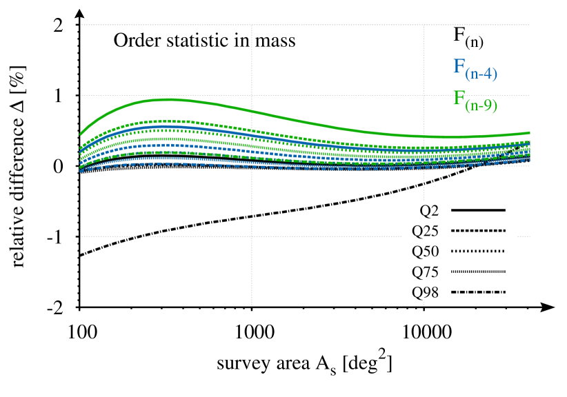
In order to determine the fitting function for the order statistics in mass, we calculate the GEV parameters according to Davis et al. (2011) and Waizmann et al. (2011) and the number of haloes, $n$, as a function of the survey area and fit them by the following functions

$$\alpha(y) =5.99888\ln(y^{0.568634}+10.5689)\,,$$ (27)

$$\beta(y) =0.362939\exp(-1.11069y^{0.324255})\,,$$ (28)

$$\gamma(y) =-0.239274\ln(y^{-0.448009}+0.747006)\,,$$ (29)

$$n(y) =10^{y+2.94112}\,,$$ (30)

where $y=\log_{10}(A_{\rm s})$. The observable $x$ in equation 26 is defined to be $x=\log_{10}(M_{200m}h)$. We present the results in Fig. 12 in the form of relative differences between the fitted and directly calculated values of five selected percentiles ($Q$2, $Q$25, $Q$50, $Q$75 and $Q$98) as a function of the survey area. The different colors denote the largest order statistics, $F_{(n)}(x)$ (black lines), the fifth largest order statistics, $F_{(n-4)}(x)$ (blue lines) and the tenth largest order statistics, $F_{(n-9)}(x)$. The relative errors in the five different percentiles are for almost the complete range of survey areas on the sub-per cent level (only $Q$98 for $F_{(n)}(x)$ exhibits a slightly larger error for very small survey areas).

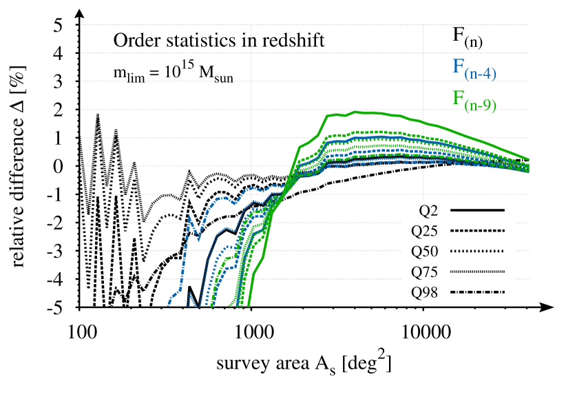
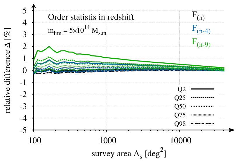
B.2 Order statistics in redshift

For fitting the order statistic in redshift, we proceed in a similar way as for the mass, setting $x=z$ in equation 26. For calculating the GEV parameters as a function of the survey area, we follow the approach presented in (Metcalf & Waizmann in preparation). However, since in contrast to the order statistics in mass, the distributions depend on the choice of the limiting survey mass, we fitted the distributions for two choices of $m_{\rm lim}$. First, we set $m_{\rm lim}=10^{15}\,M_{\odot}$, identical to the setup we discussed in this paper for the SPT massive cluster sample. Secondly, we lower the threshold to $m_{\rm lim}=5\times 10^{14}\,M_{\odot}$. In the first case, we obtain

$$\alpha(y) =1.13729\ln(0.567735y+0.332933)\,,$$ (31)

$$\beta(y) =\exp[-\exp(-1.76728y^{-1.84932}+0.929307)]\,,$$ (32)

$$\gamma(y) =-2.23597\ln(y^{-2.96376}+1.01017)\,,$$ (33)

$$n(y) =10^{0.981095y-1.52015}\,.$$ (34)

and for the second choice we find

$$\alpha(y) =2.1084\ln(0.284062y+1.09002)\,,$$ (35)

$$\beta(y) =\exp[-\exp(-0.905364y^{-0.375228}+1.30066)]\,,$$ (36)

$$\gamma(y) =-0.260275\ln(y^{-1.55487}+1.0592)\,,$$ (37)

$$n(y) =10^{0.998552y-0.451364}\,,$$ (38)

where $y=\log_{10}(A_{\rm s})$ for both cases. We present the results in Fig. 13 again as relative differences. It can be seen that in the case of high limiting mass (upper panel), the fit performs poorly for survey areas smaller than $\sim 1000\,{\rm deg}^{2}$ due to the insufficient number of haloes that are expected to be found. However, above $\sim 2000\,{\rm deg}^{2}$ the percentiles of the first ten orders can be fitted with an accuracy better than two per cent.

If the limiting mass is lowered, the quality of the fit improves drastically as shown in the lower panel of Fig. 13 for $m_{\rm lim}=5\times 10^{14}\,M_{\odot}$. In this case, sub-percent-level accuracy is reached for $A_{\rm s}\geq 1000\,{\rm deg}^{2}$ and an accuracy better than two per cent down to $100\,{\rm deg}^{2}$.

Figure 13: Relative differences, $\Delta=(Q^{\rm fit}-Q^{\rm dir})/Q^{\rm dir}$, between the fitted and directly calculated percentiles (different line styles) as a function of the survey area for the order statistics in redshift assuming $m_{\rm lim}=10^{15}\,M_{\odot}$ (upper panel) and $m_{\rm lim}=5\times 10^{15}\,M_{\odot}$ (lower panel). The differences are shown for three different ranks, the largest (black lines), the fifth largest (blue lines) and the tenth largest (green lines) one.

References

- Allen et al. (2011) Allen S. W., Evrard A. E., Mantz A. B., 2011, ARA&A, 49, 409
- Arnold et al. (1992) Arnold B. C., Balakrishnan N., Nagaraja H. N., 1992, A First Course in Order Statistics. John Wiley & Sons, New York
- Bhattacharya et al. (2011) Bhattacharya S., Heitmann K., White M., Lukić Z., Wagner C., Habib S., 2011, ApJ, 732, 122
- Cappelluti et al. (2011) Cappelluti N. et al., 2011, Memorie della Societa Astronomica Italiana Supplementi, 17, 159
- Carlstrom et al. (2011) Carlstrom J. E. et al., 2011, Publi. Astron. Soc. Pac., 123, 568
- Carlstrom et al. (2002) Carlstrom J. E., Holder G. P., Reese E. D., 2002, ARA&A, 40, 643
- Coles (2001) Coles S., 2001, An Introduction to Statistical Modeling of Extreme Values. Springer
- David & Nagaraja (2003) David H. A., Nagaraja H. N., 2003, Order Statistics. John Wiley & Sons, Hoboken, New Jersey
- Davis et al. (2011) Davis O., Devriendt J., Colombi S., Silk J., Pichon C., 2011, MNRAS, 413, 2087
- Ebeling et al. (2001) Ebeling H., Edge A. C., Henry J. P., 2001, ApJ, 553, 668
- Eddington (1913) Eddington A. S., 1913, MNRAS, 73, 359
- Fisher & Tippett (1928) Fisher R., Tippett L., 1928, Proc. Cambridge Phil. Soc., 24, 180
- Foley et al. (2011) Foley R. J. et al., 2011, ApJ, 731, 86
- Gnedenko (1943) Gnedenko B., 1943, Ann. Math., 44, 423
- Harrison & Coles (2012) Harrison I., Coles P., 2012, MNRAS, 421, L19
- Harrison & Hotchkiss (2012) Harrison I., Hotchkiss S., 2012, ArXiv e-prints
- Holz & Perlmutter (2012) Holz D. E., Perlmutter S., 2012, ApJL, 755, L36
- Hotchkiss (2011) Hotchkiss S., 2011, J. Cosmology Astroparticle Phys., 7, 4
- Hoyle et al. (2011) Hoyle B., Jimenez R., Verde L., 2011, Phys. Rev. D, 83, 103502
- Jee et al. (2009) Jee M. J. et al., 2009, ApJ, 704, 672
- Komatsu et al. (2011) Komatsu E. et al., 2011, ApJS, 192, 18
- Laureijs et al. (2011) Laureijs R. et al., 2011, preprint (arXiv: 1110.3193)
- Mahdavi et al. (2008) Mahdavi A., Hoekstra H., Babul A., Henry J. P., 2008, MNRAS, 384, 1567
- Menanteau et al. (2012) Menanteau F. et al., 2012, ApJ, 748, 7
- Meneghetti et al. (2010) Meneghetti M., Rasia E., Merten J., Bellagamba F., Ettori S., Mazzotta P., Dolag K., Marri S., 2010, A&A, 514, A93
- Mortonson et al. (2011) Mortonson M. J., Hu W., Huterer D., 2011, Phys. Rev. D, 83, 023015
- Mullis et al. (2005) Mullis C. R., Rosati P., Lamer G., Böhringer H., Schwope A., Schuecker P., Fassbender R., 2005, ApJL, 623, L85
- Navarro et al. (1996) Navarro J. F., Frenk C. S., White S. D. M., 1996, ApJ, 462, 563
- Pace et al. (2010) Pace F., Waizmann J., Bartelmann M., 2010, MNRAS, 406, 1865
- Piffaretti et al. (2011) Piffaretti R., Arnaud M., Pratt G. W., Pointecouteau E., Melin J.-B., 2011, A&A, 534, A109
- Planck Collaboration et al. (2012) Planck Collaboration et al., 2012, preprint (arXiv: 1204.2743)
- Press & Schechter (1974) Press W. H., Schechter P., 1974, ApJ, 187, 425
- Rasia et al. (2012) Rasia E. et al., 2012, New Journal of Physics, 14, 055018
- Rosati et al. (2009) Rosati P. et al., 2009, A&A, 508, 583
- Sheth & Tormen (1999) Sheth R. K., Tormen G., 1999, MNRAS, 308, 119
- Stalder et al. (2012) Stalder B. et al., 2012, preprint (arXiv: 1205.6478)
- Sunyaev & Zeldovich (1980) Sunyaev R. A., Zeldovich I. B., 1980, ARA&A, 18, 537
- Sunyaev & Zeldovich (1972) Sunyaev R. A., Zeldovich Y. B., 1972, Comments on Astrophysics and Space Physics, 4, 173
- Tauber, J. A. et al. (2010) Tauber, J. A. et al., 2010, A&A, 520, A1
- Tinker et al. (2008) Tinker J., Kravtsov A. V., Klypin A., Abazajian K., Warren M., Yepes G., Gottlöber S., Holz D. E., 2008, ApJ, 688, 709
- Voges et al. (1999) Voges W. et al., 1999, A&A, 349, 389
- Voit (2005) Voit G. M., 2005, Reviews of Modern Physics, 77, 207
- Waizmann et al. (2011) Waizmann J.-C., Ettori S., Moscardini L., 2011, MNRAS, 418, 456
- Waizmann et al. (2012a) Waizmann J.-C., Ettori S., Moscardini L., 2012a, MNRAS, 420, 1754
- Waizmann et al. (2012b) Waizmann J.-C., Ettori S., Moscardini L., 2012b, MNRAS, 422, 3554
- White (1979) White S. D. M., 1979, MNRAS, 186, 145
- Williamson et al. (2011) Williamson R. et al., 2011, ApJ, 738, 139
- Zhang et al. (2010) Zhang Y.-Y. et al., 2010, ApJ, 711, 1033