First 3D MHD simulation of a massive-star magnetosphere with application to H$\alpha$ emission from 1͡oc

Abstract

We present the first fully 3D MHD simulation for magnetic channeling and confinement of a radiatively driven, massive-star wind. The specific parameters are chosen to represent the prototypical slowly rotating magnetic O star $\theta^{1}$ Ori C, for which centrifugal and other dynamical effects of rotation are negligible. The computed global structure in latitude and radius resembles that found in previous 2D simulations, with unimpeded outflow along open field lines near the magnetic poles, and a complex equatorial belt of inner wind trapping by closed loops near the stellar surface, giving way to outflow above the Alfvén radius. In contrast to this previous 2D work, the 3D simulation described here now also shows how this complex structure fragments in azimuth, forming distinct clumps of closed loop infall within the Alfvén radius, transitioning in the outer wind to radial spokes of enhanced density with characteristic azimuthal separation of $15-20\degr$. Applying these results in a 3D code for line radiative transfer, we show that emission from the associated 3D ‘dynamical magnetosphere’ matches well the observed H$\alpha$ emission seen from $\theta^{1}$ Ori C, fitting both its dynamic spectrum over rotational phase, as well as the observed level of cycle to cycle stochastic variation. Comparison with previously developed 2D models for Balmer emission from a dynamical magnetosphere generally confirms that time-averaging over 2D snapshots can be a good proxy for the spatial averaging over 3D azimuthal wind structure. Nevertheless, fully 3D simulations will still be needed to model the emission from magnetospheres with non-dipole field components, such as suggested by asymmetric features seen in the H$\alpha$ equivalent-width curve of $\theta^{1}$ Ori C.

1 Introduction

Massive, hot (OB type) stars lack the vigorous subsurface convection thought to drive the dynamo central to the magnetic activity cycles of the sun and other cool stars. Nonetheless, new generations of spectropolarimeters have directly revealed large-scale, organized (often significantly dipolar) magnetic fields ranging in strength from 0.1 to 10 kG in several dozen OB stars (e.g. Donati et al., 2002, 2006; Hubrig et al., 2006; Petit et al., 2008; Grunhut et al., 2009; Martins et al., 2010) with ongoing monitoring and surveys carried out by the MiMeS (Magnetism in Massive Stars) consortium (Wade et al., 2012).

A key theoretical issue, examined in a series of papers (ud-Doula & Owocki, 2002; ud-Doula et al., 2008, 2009), is how such strong fields can, in combination with stellar rotation, channel and confine the radiatively driven stellar wind outflows of such OB stars, leading to the formation of a circumstellar magnetosphere. In relatively rapidly rotating magnetic Bp stars (with periods of order a day), magnetically trapped wind material above the Kepler co-rotation radius is centrifugally supported, and so builds up into a stable centrifugal magnetosphere (Townsend & Owocki, 2005), often leading to rotationally modulated, high velocity Balmer line emission (Townsend et al., 2005).

However, likely because of the angular momentum loss in their stronger magnetic winds, most O-stars with detected surface magnetic fields are slow rotators, with periods ranging from 15 days for $\theta^{1}$ Ori C to 538 days for HD 191612 and 55 years for HD 108 (Stahl et al., 2008; Howarth et al., 2007; Martins et al., 2010), implying a very limited dynamical effect of rotation on the wind magnetic channeling. Indeed, Gagné et al. (2005) showed that non-rotating, two-dimensional (2D) magnetohydrodynamic (MHD) simulations match well the temperature, luminosity, and rotational phase-dependent occultation of the X-ray emitting plasma around $\theta^{1}$ Ori C.

For the even more slowly rotating case of HD 191612, Sundqvist et al. (2012) have used similar 2D MHD simulations to show that both the strength and rotational phase variation of the observed H$\alpha$ emission can be well reproduced in terms of a dynamical magnetosphere; in this case, the higher O-star mass loss rate means that, even without significant centrifugal support, the transient magnetic suspension and subsequent gravitational infall of magnetically trapped material yields a high enough circumstellar density to give strong Balmer line emission (see also Grunhut et al. 2012 for a similar application to another O-star HD 57682).

To provide a sound basis for interpreting the Balmer emission in the growing sample of magnetic O-stars being discovered in the MiMeS project (Wade et al., 2012; Petit et al., 2012), the present paper applies this concept of a dynamical magnetosphere to analyzing the rotationally modulated H$\alpha$ line emission of the prototypical magnetic O-star $\theta^{1}$ Ori C, but now using, for the first time, fully 3D MHD simulations of the magnetic channeling and confinement of its radiatively driven stellar wind.

This extension to 3D represents a significant advance over the Sundqvist et al. (2012) approach, which was based on simulations that assume 2D axisymmetry, and so artificially suppress any variations in the azimuthal coordinate $\phi$. To mimic the expected azimuthal fragmentation of structure in a 3D model, Sundqvist et al. (2012) computed spectra from multiple snapshots of a 2D MHD simulation with large stochastic variations, which were then time-averaged as a proxy for the radiation-transport spatial averaging over azimuth in a full 3D model.

The 3D simulations here compute this lateral structure directly, applying the results to a full 3D radiative transfer model of the Balmer emission, and its variability with stochastic fluctuations of the wind, as well as with the changing observer perspective over rotational phase. The next section (§2) describes the basic MHD method, along with the parameters, boundary conditions, and numerical grid used. This leads (§3) to a general description of the resulting 3D structure and evolution, with emphasis on the dense, near-equatorial, magnetically confined gas that makes up the dynamical magnetosphere. These simulation results are then applied (§4) within full 3D radiative transfer calculations to derive the Balmer line emission and its variation. We conclude (§5) with a summary discussion of the implications for understanding the circumstellar emission of magnetic massive stars, along with an outline for future work.

2 3D Simulation Method

2.1 Basic formalism

For our 3D dynamical models we follow the basic methods and formalism developed for 2D simulations by ud-Doula & Owocki (2002), as generalized by Gagné et al. (2005) to include a detailed energy equation with optically thin radiative cooling (MacDonald & Bailey, 1981). Since 3D modeling, especially MHD, is computationally intensive, we now use the parallel version of the publicly available numerical code ZEUS-3D called ZEUS-MP (Hayes et al., 2006), which is an independent code but employs essentially the same numerical algorithms, although in a parallel programming environment.

As in ud-Doula & Owocki (2002), the treatment of radiative driving by line-scattering follows the standard Castor, Abbott & Klein (1975, hereafter CAK) formalism, corrected for the finite cone angle of the star, using a spherical expansion approximation for the local flow gradients (Pauldrach, Puls & Kudritzki, 1986; Friend & Abbott, 1986). This ignores non-radial components of the line-force that may result from velocity gradients of the flow in the lateral directions. Although in purely hydrodynamic models these forces can have significant impact, e.g. by inhibiting wind compressed disk (Owocki et al., 1996), in magnetic models they are generally small compared to the strong non-radial force components associated with the magnetic field (ud-Doula, 2003). It also ignores the extensive small-scale wind structure and clumping that can arise from the intrinsic instability of line driving (Owocki et al., 1988), since modeling such dynamics requires a non-local line-force integration that is too computationally expensive to be tractable in the 3D MHD simulations described here.

2.2 Numerical grid

The computational grid and boundary conditions are again similar to those used by ud-Doula & Owocki (2002), as generalized by ud-Doula et al. (2008) to include the non-zero azimuthal velocity at the lower boundary arising from rotation. Flow variables are specified on a fixed 3D spatial mesh in radius, co-latitude, and azimuth: $\{r_{i},\theta_{j},\phi_{k}\}$. The mesh in radius is defined from an initial zone $i=1$, which has a left interface at $r_{1}=R_{\ast}$, the star’s surface radius, out to a maximum zone ($i=n_{r}=300$), which has a right interface at $r_{300}=10R_{\ast}$. Near the stellar base, where the flow gradients are steepest, the radial grid has an initially fine spacing with $\Delta r_{1}=0.0048R_{\ast}$, and then increases by 1% per zone out to a maximum of $\Delta r_{299}=0.095R_{\ast}$. This is fine enough to resolve gradients in the subsonic base, but is larger than used in previous models; this allows for a larger time step, set as 0.3 of the Courant time, giving a typical time step of 0.1 s.

The mesh in co-latitude uses $n_{\theta}=100$ zones to span the two hemispheres from one pole, where the $j=1$ zone has a left interface at $\theta_{1}=0\degr$, to the other pole, where the $j=n_{\theta}=100$ zone has a right interface at $\theta_{100}=180\degr$. To facilitate resolution of compressed flow structure near the magnetic equator at $\theta=90\degr$, the zone spacing has a minimum of $\Delta\theta_{49}=\Delta\theta_{50}=0.29\degr$ about the equator, and then increases by 5% per zone toward each pole, where $\Delta\theta_{1}=\Delta\theta_{99}=5.5\degr$.

The mesh in azimuth is uniform, with $n_{\phi}=120$ zones of fixed size $\Delta\phi=3\degr$ over the full 360$\degr$ range. We also performed an initial test run with twice the number of azimuthal zones for our future resolution study. But preliminary results show that although there are some differences in finer structure during initial phases of breakup in azimuth, the asymptotic azimuthal structure scale is similar to that found here.

2.3 Boundary conditions

Boundary conditions are implemented by specification of variables in two phantom or ghost zones. At the outer radius, the flow is invariably super-Afvénic outward, and so outer boundary conditions for all variables (i.e. density, energy, and the radial and latitudinal components of both the velocity and magnetic field) are set by simple extrapolation assuming constant gradients. On the other hand, at the inner radius, where the surface of the star is defined, the flow is sub-Afvénic. In general, the number of characteristics pointing into the grid determines the number of boundary conditions needed to be specified (Bogovalov, 1997). For supermagnetosonic flow, this implies that all seven variables (density, internal energy or pressure, three components of velocity and two transverse components of the magnetic field) must be specified. But for sub-magnetosonic flow here, only four characteristics point into the grid (entropy, fast, slow and Afvénic). Thus, four variables must be specified and the remaining three of the variables need to be extrapolated (Bogovalov, 1997). These conditions are briefly described below.

In the two radial zones below $i=1$, we set the radial velocity $v_{r}$ by constant-slope extrapolation, and fix the density at a value $\rho_{o}$ chosen to ensure subsonic base outflow for the characteristic mass flux of a 1D, nonmagnetic CAK model, i.e. $\rho_{o}\approx{\dot{M}}/(4\pi R_{\ast}^{2}a/6)$. These conditions allow the mass flux and the radial velocity to adjust to whatever is appropriate for the local overlying flow (Owocki, Castor, and Rybicki 1988). In most zones, this corresponds to a subsonic wind outflow, although inflow at up to the sound speed is also allowed.

Magnetic flux is introduced through the lower boundary as the radial component of a dipole field $B_{r}(R_{\ast},\theta)=B_{o}\cos(\theta)$, where the polar field $B_{o}=1100$ G is adopted from the observationally inferred value for $\theta^{1}$ Ori C (Donati et al., 2002). The latitudinal components of magnetic field, $B_{\theta}$, and flow speed $v_{\theta}$, are again set by constant slope extrapolation. The azimuthal field $B_{\phi}$ is likewise set by extrapolation, while the azimuthal speed is set by the assumed stellar rotation, $v_{\phi}(R_{\ast},\theta)=V_{rot}\sin\theta$.

While the code is fully 3D, the choice of spherical coordinates leads to numerical difficulties near the coordinate singularity along the polar axis, which is treated with reflecting boundary conditions. Because this prohibits any flow across the axis, we ignore the slow, oblique rotation inferred for $\theta^{1}$ Ori C, since at a period of $\sim$15 d, it is dynamically unimportant. However, to avoid pockets of rarefied gas near the stellar surface that lead to very small Courant time, we do introduce a small dynamically insignificant field-aligned rotation with an equatorial surface speed $V_{rot}=10\,{\rm km\,s^{-1}}$.

2.4 Stellar parameters and initial condition

The adopted stellar and wind parameters are summarized in Table 1. Using these parameter values, we first relax a non-magnetic, spherically symmetric wind model to an asymptotic steady state; this yields the quoted mass loss rate and terminal speed, which are in very good agreement with the standard CAK scaling, adjusted for a finite-disk and non-zero sound speed (Owocki & ud-Doula 2004). This relaxed CAK steady state is used for the initial condition in density and velocity. The temperature is initially set to the associated stellar effective temperature, $T_{\rm eff}\approx 40,000$ K, which also subsequently sets a floor for the temperature, to approximate a radiative equilibrium in which photoionization heating counters the cooling by line emission and adiabatic expansion.

The magnetic field is initialized to have a simple dipole form with components $B_{r}=B_{o}(R_{\ast}/r)^{3}\cos\theta$, $B_{\theta}=(B_{o}/2)(R_{\ast}/r)^{3}\sin\theta$, and $B_{\phi}=0$, with $B_{o}$ the polar field strength at the stellar surface. From this initial condition, the numerical model is then evolved forward in time to study the dynamical competition between the field and flow, as detailed in §3.

Table 1: Stellar and wind parameters

Name	Parameter	Value
Mass	$M_{\ast}$	$40M_{\odot}$
Radius	$R_{\ast}$	$8R_{\odot}$
Luminosity	$L_{\ast}$	$1.5\times 10^{5}L_{\odot}$
CAK $\alpha$	$\alpha$	0.5
Line strength	$\bar{Q}$	700
Mass loss rate	$\dot{M}$	$3.3\times 10^{-7}M_{\odot}$yr-1
Terminal speed	$V_{\infty}$	$3200$ km s-1
Polar field	$B_{Pole}$	$1100$ G

Following ud-Doula & Owocki (2002), the stellar, wind, and magnetic parameters in Table 1 can be used to define a dimensionless “wind magnetic confinement parameter”,

$$\eta_{\ast}\equiv\frac{B_{eq}^{2}R_{\ast}^{2}}{{\dot{M}}V_{\infty}}\approx 14\,,$$ (1)

where for a dipole, the equatorial field is just half the polar value, $B_{eq}=B_{o}/2$. Since $\eta_{\ast}>1$, the magnetic field dominates the wind outflow near the stellar surface. But because the magnetic energy density has a much steeper radial decline ($B^{2}\sim r^{-6}$ for a dipole) than the wind ($\rho v^{2}\sim r^{-2}$ if near terminal speed), the wind can strip open field lines above a a characteristic Alfvén radius, set approximately by (ud-Doula et al., 2008)

$$\frac{R_{\rm A}}{R_{\ast}}\approx 0.3+\eta_{\ast}^{1/4}\approx 2.23\,.$$ (2)

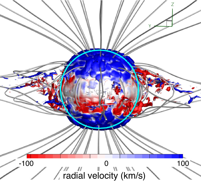
Figure 1: A near stellar surface view of an iso-density ($\log\rho=-12.5$ in cgs units) surface, colored with radial velocity $v_{r}$, ranging from $-100\,{\rm km\,s^{-1}}$ (red) to $+100\,{\rm km\,s^{-1}}$ (blue). Note how some of the gas material within the closed loop region falls back onto the stellar surface, while material in the open field (polar) region streams radially outward. The slowly moving (or infalling) region depicted as white (red) color indicates the lateral extent of the magnetosphere. The circle (cyan) represents the stellar surface.

3 MHD Simulation Results

3.1 Snapshot of 3D structure

As background for the Balmer emission line computations in §4, let us here characterize the spatial structure and time evolution resulting from our 3D MHD simulation.

The characteristic time for the CAK wind here to flow from the sonic point near the stellar surface to the outer boundary at $10R_{\ast}$ is about $t_{flow}\approx 25$ ks. For MHD simulations we find in practice (ud-Doula & Owocki, 2002) it takes $\sim 10-15$ such flow times for resulting structure to reach a state that is independent of the initial conditions. To provide an extended sampling of random variations in this asymptotic state, we run the 3D simulations here to a final time $t=1000$ ks, corresponding to roughly 40 wind flow times.

Figure 1 shows a close-in, equatorial view of the dichotomy between open field over the poles and closed loops around the equator, with density rendered as an iso-density surface for $\log\rho=-12.5$ g/cm³. The color represents the associated radial (in grid coordinate system) component of the flow velocity, ranging from -100 ${\rm km\,s^{-1}}$ inflow (red) to +100 ${\rm km\,s^{-1}}$ outflow (blue). Note that the polar regions have mainly just outflow, reflecting the open nature of the field. In contrast, the equatorial regions have a complex combination of outflow and inflow, reflecting the trapping of the underlying base wind within closed loops, with subsequent gravitational fall-back onto the stellar surface.

A similar pattern of wind trapping and subsequent infall was also seen in 2D simulations (ud-Doula & Owocki, 2002; ud-Doula et al., 2008), manifested there by a complex ‘snake’ pattern extending over radius and latitude, but formally coherent in azimuth within the imposed 2D axisymmetry. This 3D simulation now shows how, because of spontaneous symmetry breaking, this infall becomes azimuthally fragmented into multiple, dense, infalling clumps, distributed in both latitude and azimuth on a scale that is comparable to the latitudinal scale of the 2D snakes.

To provide a more complete picture of this complex, 3D wind structure, figure 2 shows both equatorial (top) and polar (bottom) views for two values of the iso-density surface, namely $\log\rho=-12.5$ (left) and $\log\rho=-13$ (right), again with the same color coding for radial velocity. The polar view now shows clearly the azimuthal organization and scale of the trapped equatorial structure, and how it becomes extended outward into radial “spokes”. While complex, the lower iso-density plot on the right shows a general trend from dominance of infall in the inner region (marked by red) to outflow at larger radii (marked by blue).

Overall, this represents a 3D generalization of the dynamical magnetosphere concept developed to characterize 2D simulations, and their application to modeling Balmer line emission (Sundqvist et al., 2012). The essential feature is that the trapping and compression of wind material in closed loops results in a substantial enhancement of the time-averaged density near the magnetospheric equator, leading then to an associated enhancement in line emission, as we demonstrate quantitatively in §4.

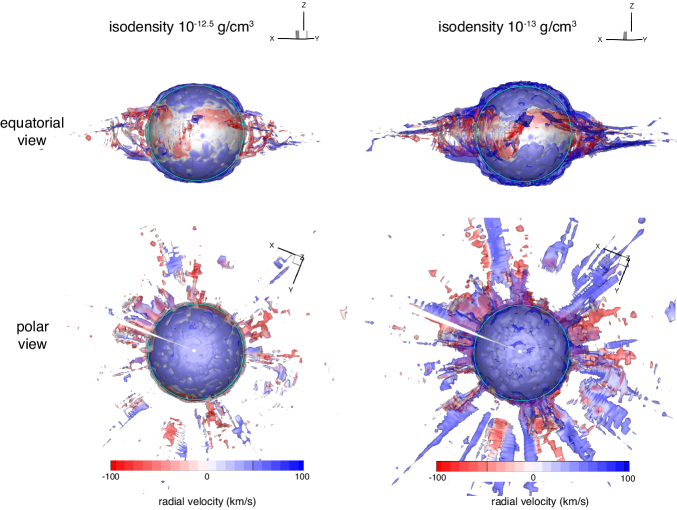
Figure 2: Iso-density surfaces at log($\rho$)=-12.5 (left) and log($\rho$)=-13.0 (right) for a fixed time snaphot $t=1$ Ms, viewed from the equator (top panels) or pole-on (bottom panels). As in figure 1, the color represents radial velocity. The equatorial ‘belt’ visible as white band (low velocity) represents the latitudinal extent of the magnetosphere. Note that substantial material within that region is falling back onto the stellar surface, thus forming the dynamical magnetosphere. The cyan circle again represents the stellar surface.

3.2 Time development and evolution of wind structure

Let us next consider how such complex spatial structure develops from the steady, spherical initial condition, and how it subsequently evolves into a stochastic variation associated with wind trapping, breakout, and infall. Since much of the key structure is near the magnetic equator, let us follow the approach developed by ud-Doula et al. (2008) that defines a radial mass distribution $dm_{\rm e}/dr$ within a specified co-latitude range $\Delta\theta$ (taken here to be $10\degr$) about the equator,

$$\frac{dm_{\rm{e}}(r,\phi,t)}{dr}\equiv 2\pi r^{2}\int_{\pi/2-\Delta\theta/2}^{\pi/2+\Delta\theta/2}\,\rho(r,\theta,\phi,t)\,\sin\theta\,d\theta\,.$$ (3)

In previous 2D models, the imposed axisymmetry means this $dm_{\rm e}/dr$ is a function of just radius and time, and so can be conveniently rendered as a colorplot to show the time and spatial variation of the equatorial material. In the present 3D case, there is an added dependence on the azimuthal coordinate $\phi$, but upon averaging over this, we again obtain a function of just radius and time,

$$\frac{d{\bar{m}}_{\rm{e}}(r,t)}{dr}\equiv\frac{1}{2\pi}\int_{0}^{2\pi}\frac{dm_{\rm e}}{dr}(r,\phi,t)\,d\phi\,.$$ (4)

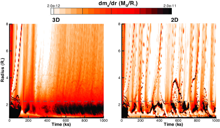
Figure 3: Equatorial mass distribution $dm_{\rm e}/dr$ (in units $M_{\odot}/R_{\ast}$) for the azimuthally averaged 3D model (left) and for a corresponding 2D model (right), plotted versus radius and time, with the dashed horizontal line showing the Alfvèn radius $R_{\rm A}\approx 2.23R_{\ast}$. Following a similar adjustment to the initial condition, the long-term evolution of the 2D models is characterized by a complex pattern of repeated strings of infall, whereas the 3D azimuthally averaged model settles into a relatively smooth asymptotic state characterized by an enhanced mass near and below the Alfvén radius.

Figure 3 compares the time and radius variation of the $d{\bar{m}}_{\rm e}/dr$ from the 3D simulation (left) with the corresponding $dm_{\rm e}/dr$ from an analogous 2D model (right) with identical parameters. The dashed horizontal line, marking the estimated Alfvén radius $R_{\rm A}\approx 2.23R_{\ast}$, roughly separates the regions of outflow along open field lines above $R_{\rm A}$, from the complex pattern of upflow and downflow for material trapped in closed magnetic loops below $R_{\rm A}$. In the 2D models, the complex infall pattern occurs in distinct, snakelike structures, but in the 3D models, these break up into multiple azimuthal fragments that, upon averaging, give the 3D panel a smoother, more uniform variation. More importantly, note the clear enhancement in the mass just below the Alfvén radius, representing what we characterize here as the dynamical magnetosphere.

To illustrate the time evolution of the azimuthal breakup and variation in 3D wind structure, the upper panels of figure 4 use a “clock format” to show the time progression of an arbitrary 36$\degr$ segment of $dm_{\rm e}/dr(r,\phi,t)$ at time steps of 50 ks, ranging over $t=50-500$ ks for the left panel, and continuing through $t=550-1000$ ks in the right panel. Following the spherically symmetric initial condition, the magnetic field first channels the wind into a compressed, azimuthally symmetric, disk-like structure ($t=50~{}\&~{}100$ ks), which however then breaks up (by $t=150$ ks) to a series of radial spokes with an azimuthal separation of roughly $\Delta\phi\approx 15-20\degr$. Remarkably, following this initial breakup, the azimuthal structure keeps the same overall character and scale within a complex stochastic variation.

Note in particular that the structure over the full $360\,\degr$, as shown for the final time $t=1000$ ks in the lower row of figure 4, is quite similar to that shown for the evolving segments in the right-side upper row for $t=550-1000$ ks. Moreover, the $\sim 500$ ks lower bound for this settling time corresponds to the time in figure 3 for the formation of the enhanced $dm_{\rm e}/dr$ that characterizes the dynamical magnetosphere.

As noted in §3.1, the inferred azimuthal scale of $15-20\degr$ is comparable to the scale of infalling “snakes” found in 2D simulations, which typically extend over some fraction of the loop length between closed footpoints. For the present case, the maximum latitude of a closed loop is about $45\degr$, giving a typical angle extent of about $15-20\degr$ for both the snakes and the azimuthal breakup. Future studies should examine whether these structure scales do in fact follow the expected loop closure latitude, which should scale with magnetic confinement parameter as $\arcsin{\eta_{\ast}^{-1/8}}$.

In summary, the equatorial structures seen in previous 2D models now become azimuthally fragmented with a characteristic separation of $\Delta\phi\approx 15-20\degr$, which however upon averaging in azimuth, have a radial and latitudinal variation that is similar to what is obtained from time-averaging in 2D models. This has important implications for modeling the associated Balmer line emission, as we discuss next.

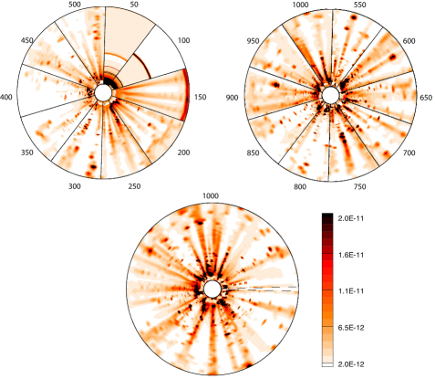
Figure 4: Time evolution of $dm_{\rm e}/dr$ for an arbitrary $36\,\degr$ azimuthal segment of the 3D model, at marked time intervals of 50 ks ranging over $t=50-500$ ks in the upper left panel, extending to $t=550-1000$ ks in the upper right. The bottom panel shows the full variation over $360\,\degr$ for the final simulation time $t=1$ Ms. As in figure 3, the units of $dm_{\rm e}/dr$ are $M_{\odot}/R_{\ast}$.

4 Balmer line emission: model vs. observations

Now let us examine to what extent the 3D MHD wind simulations presented here can reproduce the observed H$\alpha$ emission and variability in $\theta^{1}$ Ori C.

Applying the 3D radiative transfer method developed by Sundqvist et al. (2012) to the 3D MHD simulations described above, we compute synthetic H$\alpha$ profiles by solving the formal integral of radiative transfer in a cylindrical coordinate system aligned toward the observer. The angle $\alpha$ defines the observer’s viewing angle with respect to the magnetic pole, and, for given inclination $i$ and obliquity $\beta$,

$$\cos\alpha=\sin i\sin\beta\cos\Phi+\cos i\cos\beta$$ (5)

gives the observer’s viewing angle as a function of rotation phase $\Phi$. Due to the slow rotation of the targeted star, we may neglect any dynamical effects of rotation and use the same simulation for all obliquity angles $\beta$. The computations further use a pre-specified photospheric line profile as a lower boundary condition, and solve the equations of radiative transfer only in the circumstellar structure. Hydrogen NLTE departure coefficients are estimated from a spherically symmetric unified model atmosphere calculation (using fastwind, Puls et al. 2005). Moreover, since the energy equation in the MHD simulation gives only a rough estimate of the wind temperature structure, we also take this from the fastwind model, except for in shock-heated regions with $T>10^{5}$, where we set the H$\alpha$ source function and opacities to zero. For further discussion about these and other assumptions entering the Balmer line profile calculations, see Sundqvist et al. (2012) and references therein.

4.1 Periodic rotational phase variability

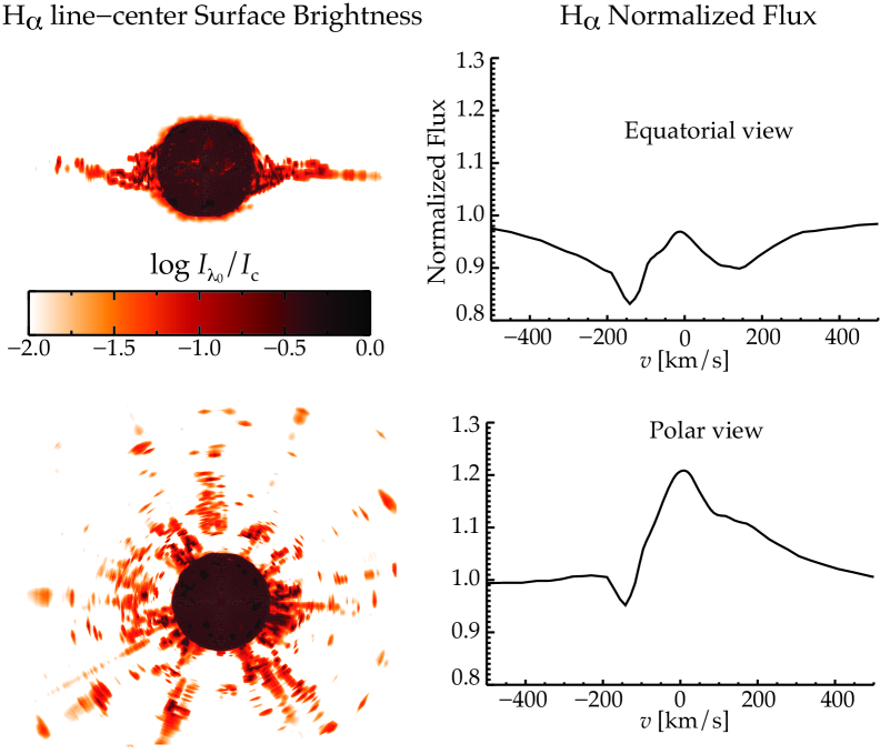
Figure 5: Synthetic H$\alpha$ surface brightness maps (left panels) and flux profiles (right panels) for observer viewing angles above the equator (upper panels) and magnetic pole (lower panels), as calculated from a snapshot of the 3D MHD wind simulation taken at 1000 ksec after initialization.

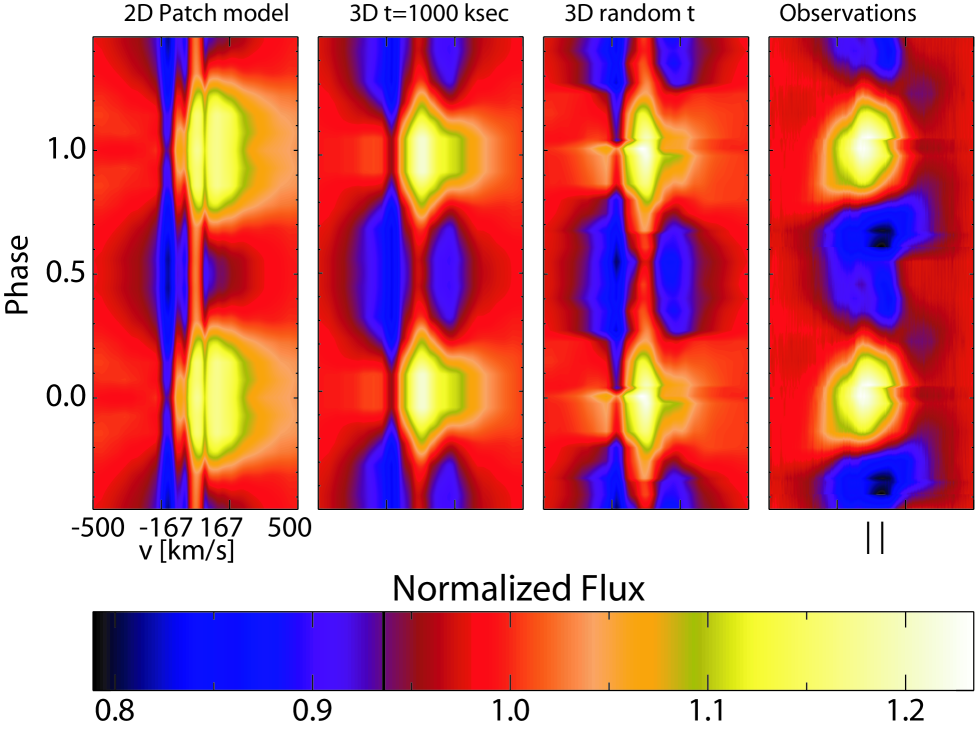
Figure 6: Observed and synthetic H$\alpha$ dynamic spectra of $\theta^{1}$ Ori C. Synthetic spectra calculated from patching together 2D model snapshots (panel 1), a single 3D model snapshot (panel 2), and from a random selection of 3D snapshots (panel 3). The vertical small lines in panel 4 represent the velocity range of the nebular emission.

Figure 5 displays synthetic H$\alpha$ line-center surface brightness maps and flux profiles viewed from above the magnetic pole and equator, corresponding approximately to rotational phases of 0.0 and 0.5, respectively, according to the ephemeris of Stahl et al. (2008). As in Sundqvist et al. (2012), we interpret the H$\alpha$ variability within the framework of a dynamical magnetosphere, but now using the full 3D dynamical model for the azimuthal wind structure. For the pole-on view, the surface brightness of line-center emission in the lower panel of figure 5 follows closely the lateral fragmentation seen from the corresponding iso-density plots in the bottom row of figure 2. Similarly, there is a good correspondence for the equatorial view, but now the projection leads to an overall lower level of the total emission, associated with the smaller projected surface area of the structure. As shown by the right panels of figure 5, this leads to a stronger level of emission in the line profiles for the polar view. But note that even for the equatorial view, the circumstellar emission still partially refills the photospheric absorption profile. Most of the emission arises from the relatively dense material trapped in the closed loops near the stellar surface, with only about 10-20% arising from the extended radial spokes. Overall, the magnetospheric structures found here have quite different morphology from compressive structures generated by instabilities of line-driving in non-magnetic stars (Feldmeier et al., 1997; Dessart & Owocki, 2003).

Within the context of the MiMeS project, 18 high-resolution, high-SNR observations of $\theta^{1}$ Ori C were obtained with the spectropolarimeter ESPaDOnS at the Canada-France-Hawaii telescope (4 from Petit et al. (2008) and 14 from MiMeS) which were used to produce the dynamical spectra of H$\alpha$ shown in figure 6. Leveraging the high spectral resolution (4 km s^-1), we remove the strong nebular line by fitting a polynomial curve to the adjacent sides of the line profile. This procedure provides us with an indication of how smoothly these lines vary in phase. Nonetheless, localised features within this velocity range (illustrated by small vertical lines in the fourth panel in figure 6) could still be hidden.

Figure 6 compares observed dynamic H$\alpha$ spectra of $\theta^{1}$ Ori C over its rotational phase (far right) with 3 models that each assume $i=\beta=45\degr$, but which have increasing levels of sophistication progressing from left to right.

The first panel is computed from 100 randomly selected 2D simulation snapshots that have been patched together to form an ‘orange slice’ pseudo-3D model with an azimuthal coherence of 3.6$\degr$. This patch approach is similar to that used to reproduce periodic H$\alpha$ variability in the magnetic O-stars HD 191612 and HD 57682 from 2D MHD simulations (Sundqvist et al., 2012; Grunhut et al., 2012).

The second panel then displays spectra computed from a single snapshot of the 3D simulation, and illustrates that such full 3D model spectra are in fact qualitatively very similar to the averaged 2D models, as was suggested by Sundqvist et al. (2012).

Finally, the third panel in Figure  6 is constructed from a random selection of 3D snapshots with phases that coincide with the observations seen in the fourth panel; it is discussed further in the following subsection.

Overall, all three models give reasonable and comparable agreement with the observed dynamic spectrum. This suggests that one can indeed use the more simplified approaches to explore how observational diagnostics constrain the properties of a dynamical magnetosphere, calibrated with selected comparisons with more computationally demanding, and physically realistic 3D models.

Although the simulations reproduce quite well both the magnitude and phase of the observed rotational variation, the observed profiles exhibit an asymmetry about phase 0.5 that is not found in our numerical models; such asymmetries may have their origin in, e.g., non-dipolar components of the magnetic field, consideration of which we defer to future study. Moreover, to match the absolute level of emission, we have increased the H$\alpha$ scaling invariant $\sqrt{f_{\rm cl}}\dot{M}/(v_{\infty}R_{\star})^{3/2}$ of the underlying simulations by a factor of 2.5, where $f_{\rm cl}$ is an overdensity correction factor that accounts for small-scale clump structure (e.g., Puls et al., 2008). The need for this increase may indicate the MHD simulations either assume a somewhat too low mass-loss rate for $\theta^{1}$ Ori C, or underestimate the overdensities of the emitting H$\alpha$ material around the magnetic equator.

4.2 Stochastic short time-scale variability

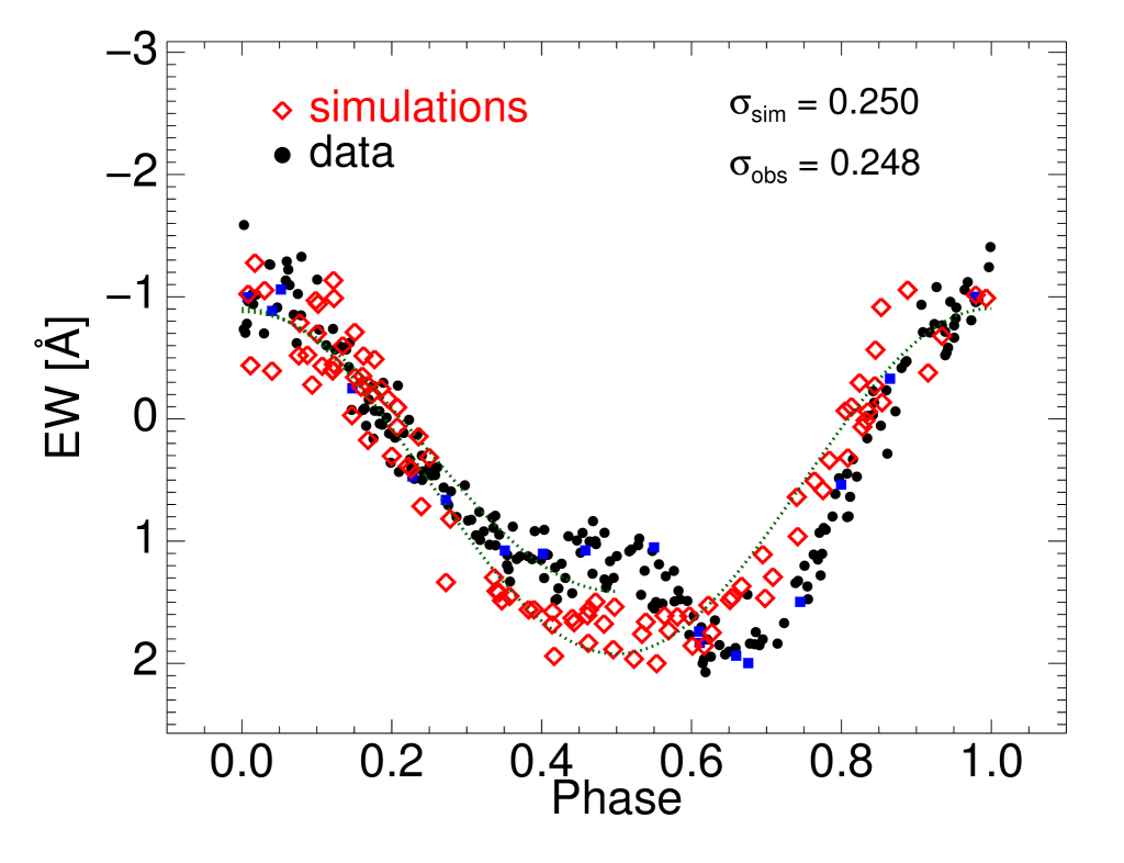
Figure 7: Observed and synthetic H$\alpha$ equivalent-width curves. The synthetic measurements are calculated from 100 random 3D simulation snapshots phased randomly. The quoted $\sigma$’s measure standard deviations from functional fits (dotted green lines) to simulations and data. The blue squares denote the additional observational data points that correspond to the dynamical spectra in figure 6. See text.

The H$\alpha$ emission of $\theta^{1}$ Ori C has been monitored regularly for nearly two decades and an extensive set of equivalent width measurements has been compiled by Stahl et al. (2008) shown as the black dots in figure 7, phased according to the 15.4 d rotation period using the ephemeris of Stahl et al. (2008). Although the level of both emission and its modulation with rotational phase are very stable, there is some significant random variability present during all phases. Such stochastic H$\alpha$ scatter may originate from small differences in the amount of material trapped in the dynamical magnetosphere at any given time.

To examine the level of such short time-scale variability in our 3D MHD model, we randomly select simulation snapshots between 800-1000 ksec and from these calculate line profiles for random rotational phases. The results show that the model closely reproduces both the systematic variation with rotational phase, as well as the stochastic deviation in the multi-year data from the mean at each phase. The quoted standard deviations $\sigma_{\rm sim}\approx\sigma_{\rm obs}\approx 0.25\,\rm\AA$ have been estimated by calculating the variance from separate functional fits $f(\alpha)=a+b|\cos\alpha|$ to the model and observational data. (Due to the asymmetry, data are fit only between phases 0 and 0.5.) Though the interpretation of this simple estimate is complicated by the fact that non-magnetic O-stars with significant wind strength also show stochastic H$\alpha$ variability (Markova et al., 2005), it nevertheless suggests that in $\theta^{1}$ Ori C the observed H$\alpha$ scatter is likely dominated by processes associated with the star’s dynamical magnetosphere.

This approach of randomizing variations in model equivalent width can also be used to account for the effect of stochastic wind variations on the synthetic dynamic spectrum, as illustrated in the third panel of figure 6. We have aligned synthetic model phases to those for the subset of times with available spectra from our MiMeS observations (blue squares in figure 7). Comparison of the third and fourth panels of figure 6 again show an overall good agreement between the models and observations.

5 Discussion, Conclusions and Future Work

A central advance of the work described here is the incorporation of all three spatial dimensions in the MHD simulation model. This allows us to follow directly the spontaneous breaking of the azimuthal symmetry that was imposed in previous 2D models, while still confirming a global structure that is quite similar to that found in those models. At high latitude this is characterized by fast wind outflow along open field lines. At low latitudes, an equatorial belt of closed loops traps the wind into a complex pattern of upflow and infall near the star, but this gives way again to open field outflow above the Alfvén radius.

The addition of a third dimension along the azimuth means that this complex pattern now fragments into distinct regions of upflowing wind and infalling clumps. This leads to an associated fragmentation of the wind breakout above the Alfvén radius, resulting in an alternating pattern of radial spokes of slow, high-density outflow, with a characteristic azimuthal separation of $15-20\degr$, divided roughly equally between the dense spokes and a more rarefied flow between them. Such a separation angle is well above the adopted azimuthal grid size $\Delta\phi\approx 3\degr$, and indeed a higher resolution test run with half this grid size gives asymptotic wind structure at a similar scale. As such, this scale does not appear to be strongly dependent on the grid resolution, though further investigation will be needed to test this and clarify what physical processes set the structure size.

An additional focus here is the application of these 3D MHD simulation results to modeling the H$\alpha$ line emission from the prototypical magnetic massive star $\theta^{1}$ Ori C, representing a 3D extension of the dynamical magnetosphere paradigm recently introduced by Sundqvist et al. (2012). As a proxy for the spatial averaging over the azimuthal variations expected from a full 3D model, this previous work computed time-averaged spectra from a strictly 2D axisymmetric simulations with stochastically varying wind structure. As demonstrated by the close similarity of the 2D vs. 3D models for the dynamic spectra in figure 6, a key result here is to confirm a general validity for this proxy approach. This suggests then that future modeling of such rotational variation of line emission in the growing number of slowly rotating magnetic O-type stars could be achieved with reasonable accuracy using much less computationally expensive 2D MHD simulations to characterize the dynamical magnetosphere. Of course, such an approach is only possible for the simple, axisymmetric field configuration of a magnetic dipole. To account for deviations from a dipole, such as might be inferred from the asymmetric phase variation in the equivalent width light curve here, one will again need to carry out fully 3D simulations.

Apart from this modest non-dipole asymmetry, both the 2D and 3D dipole-based models here match quite well the rotational phase variation of H$\alpha$. But a further quite remarkable result of the present study is how well the synthetic 3D, “random time” model (third panel in figure 6) reproduces also the observed stochastic variation in the H$\alpha$ equivalent width, as demonstrated in figure 7. This suggests that the number and sizes of distinct structures generated in the simulated dynamical magnetosphere may be quite comparable to that in the actual star.

On the other hand, the magnetic O-star HD 191612, which has a stronger magnetic confinement ($\eta_{\ast}\approx 50$), shows a distinctly lower level of such random variation in H$\alpha$ equivalent width (Howarth et al., 2007). This suggests that the general number and size of structures may depend on, e.g., the size or rigidity of the magnetosphere. This again requires further investigation through a systematic parameter study.

Finally, while the overall agreement between 3D model predictions and observed H$\alpha$ variations is quite good, this is achieved with a modest adjustment in the assumed mass loss rate and/or wind clumping factor. Future work should examine the role of the line-deshadowing instability in inducing clumping in the wind acceleration region, and how well the numerical grid resolves this and other small-scale flow structures arising from wind compression in closed magnetic loops. In addition, future 3D models should consider both dipolar and non-dipolar field topologies that are not aligned to the rotation axis. In summary, while the results here have provided an encouraging first step, there remains much work to develop realistic 3D models of the magnetospheres and channeled wind outflows from magnetic massive stars.

References

- Bogovalov (1997) Bogovalov S. V., 1997, A&A, 323, 634
- Castor et al. (1975) Castor J. I., Abbott D. C., Klein R. I., 1975, ApJ, 195, 157
- Dessart & Owocki (2003) Dessart L., Owocki S. P., 2003, A&A, 406, L1
- Donati et al. (2002) Donati J.-F., Babel J., Harries T. J., Howarth I. D., Petit P., Semel M., 2002, MNRAS, 333, 55
- Donati et al. (2006) Donati J.-F., Howarth I. D., Bouret J.-C., Petit P., Catala C., Landstreet J., 2006, MNRAS, 365, L6
- Feldmeier et al. (1997) Feldmeier A., Puls J., Pauldrach A. W. A., 1997, A&A, 322, 878
- Friend & Abbott (1986) Friend D. B., Abbott D. C., 1986, ApJ, 311, 701
- Gagné et al. (2005) Gagné M., Oksala M. E., Cohen D. H., Tonnesen S. K., ud-Doula A., Owocki S. P., Townsend R. H. D., MacFarlane J. J., 2005, ApJ, 628, 986
- Grunhut et al. (2009) Grunhut J. H., Wade G. A., Marcolino W. L. F., Petit V., Henrichs H. F., Cohen D. H., Alecian E., Bohlender D., Bouret J.-C., Kochukhov O., Neiner C., St-Louis N., Townsend R. H. D., 2009, MNRAS, 400, L94
- Grunhut et al. (2012) Grunhut J. H., Wade G. A., Sundqvist J. O., ud-Doula A., Neiner C., Ignace R., Marcolino W. L. F., Rivinius T., Fullerton A., Kaper L., Mauclaire B., Buil C., Garrel T., Ribeiro J., Ubaud S., the MiMeS Collaboration 2012, MNRAS, in press
- Grunhut et al. (2012) Grunhut et al. 2012, MNRAS, in press
- Hayes et al. (2006) Hayes J. C., Norman M. L., Fiedler R. A., Bordner J. O., Li P. S., Clark S. E., ud-Doula A., Mac Low M.-M., 2006, ApJS, 165, 188
- Howarth et al. (2007) Howarth I. D., Walborn N. R., Lennon D. J., Puls J., Nazé Y., Annuk K., Antokhin I., Bohlender D., Bond 2007, MNRAS, 381, 433
- Hubrig et al. (2006) Hubrig S., Briquet M., Schöller M., De Cat P., Mathys G., Aerts C., 2006, MNRAS, 369, L61
- MacDonald & Bailey (1981) MacDonald J., Bailey M. E., 1981, MNRAS, 197, 995
- Markova et al. (2005) Markova N., Puls J., Scuderi S., Markov H., 2005, A&A, 440, 1133
- Martins et al. (2010) Martins F., Donati J.-F., Marcolino W. L. F., Bouret J.-C., Wade G. A., Escolano C., Howarth I. D., Mimes Collaboration 2010, MNRAS, 407, 1423
- Owocki et al. (1988) Owocki S. P., Castor J. I., Rybicki G. B., 1988, ApJ, 335, 914
- Owocki et al. (1996) Owocki S. P., Cranmer S. R., Gayley K. G., 1996, ApJ, 472, L115+
- Pauldrach et al. (1986) Pauldrach A., Puls J., Kudritzki R. P., 1986, A&A, 164, 86
- Petit et al. (2008) Petit V., Wade G. A., Drissen L., Montmerle T., Alecian E., 2008, MNRAS, 387, L23
- Petit et al. (2012) Petit et al. 2012, MNRAS, in preparation
- Puls et al. (2005) Puls J., Urbaneja M. A., Venero R., Repolust T., Springmann U., Jokuthy A., Mokiem M. R., 2005, A&A, 435, 669
- Puls et al. (2008) Puls J., Vink J. S., Najarro F., 2008, A&AR, 16, 209
- Stahl et al. (2008) Stahl O., Wade G., Petit V., Stober B., Schanne L., 2008, A&A, 487, 323
- Sundqvist et al. (2012) Sundqvist J. O., ud-Doula A., Owocki S. P., Townsend R. H. D., Howarth I. D., Wade G. A., 2012, MNRAS, 423, L21
- Townsend & Owocki (2005) Townsend R. H. D., Owocki S. P., 2005, MNRAS, 357, 251
- Townsend et al. (2005) Townsend R. H. D., Owocki S. P., Groote D., 2005, ApJ, 630, L81
- ud-Doula (2003) ud-Doula A., 2003, PhD thesis, University of Delaware
- ud-Doula & Owocki (2002) ud-Doula A., Owocki S. P., 2002, ApJ, 576, 413
- ud-Doula et al. (2008) ud-Doula A., Owocki S. P., Townsend R. H. D., 2008, MNRAS, 385, 97
- ud-Doula et al. (2009) ud-Doula A., Owocki S. P., Townsend R. H. D., 2009, MNRAS, 392, 1022
- Vink et al. (2001) Vink J. S., de Koter A., Lamers H. J. G. L. M., 2001, A&A, 369, 574
- Wade et al. (2012) Wade G. A., Grunhut J. H., the MiMeS Collaboration 2012, ArXiv e-prints