Adaptive Differential Feedback in Time-Varying Multiuser MIMO Channels

Abstract

In the context of a time-varying multiuser multiple-input-multiple-output (MIMO) system, we design recursive least squares based adaptive predictors and differential quantizers to minimize the sum mean squared error of the overall system. Using the fact that the scalar entries of the left singular matrix of a Gaussian MIMO channel becomes “almost” Gaussian distributed even for a small number of transmit antennas, we perform adaptive differential quantization of the relevant singular matrix entries. Compared to the algorithms in the existing differential feedback literature, our proposed quantizer provides three advantages: first, the controller parameters are flexible enough to adapt themselves to different vehicle speeds; second, the model is backward adaptive i.e., the base station and receiver can agree upon the predictor and variance estimator coefficients without explicit exchange of the parameters; third, it can accurately model the system even when the correlation between two successive channel samples becomes as low as 0.05. Our simulation results show that our proposed method can reduce the required feedback by several kilobits per second for vehicle speeds up to 20 km/h (channel tracker) and 10 km/h (singular vector tracker). The proposed system also outperforms a fixed quantizer, with same feedback overhead, in terms of bit error rate up to 30 km/h.

I Introduction

The advantages of multiuser multiple-input-multiple-output (MIMO) has led to its inclusion in the standard proposals for fourth generation wireless systems, e.g., mobile WiMax [1]. The best MIMO system performance can be achieved when channel state information (CSI) is available at the transmitter [2]. In a frequency division duplexing system, downlink CSI needs to be estimated at the receiver, quantized and provided to the base station via an uplink feedback channel. Recent work suggests that this might also be required in broadband time division duplex systems [3]. Therefore, reducing feedback overhead while providing accurate CSI plays an important role in multiuser transceiver design. In the available literature, scalar quantization (SQ) [4, 5], vector quantization (VQ) [6] and matrix quantization [7] have all been used to quantize CSI. SQ has been included in several standards (e.g.IEEE 802.11n [8]) due to its linear computational complexity. This paper focuses on the reduction of feedback overhead in time varying channels that employs SQ. We assume perfect channel estimation and delay-free noiseless feedback and focus on quantization only.

The feedback overhead can be significantly reduced using differential feedback by exploiting temporal correlation of the channel [9, 10, 11]. Most of these works model the channel as a first order Gauss-Markov process and use a fixed differential quantizer. The authors assume that the transmitter and receiver agree on the value of the parameters in the Markov chain. Since this assumption does not hold in non-stationary channels, there has been some research in adaptive delta-modulation (ADM) based feedback [4, 5]. Both these works quantize the difference between the previous and current samples with a one-bit quantizer. However, the authors give suitable step size controller parameters for pedestrian velocities (up to 4 km/h) only.

The lack of flexibility of the available differential feedback methods motivates us to investigate adaptive differential feedback in time-varying multiuser channels. This paper makes the following two contributions: First, based on the linear least square (LLS) based adaptive differential speech quantizer model proposed by Stroh [12], we develop a 2-bit recursive least square (RLS) adaptive differential feedback in a time-varying environment. Second, we design RLS adaptive tracking of the singular vector entries of each users’ channel matrix and show that, if the number of data streams is less than the total number of receive antennas, this method reduces feedback overhead. Both these methods can lead to reducing the required feedback overhead by several kBits/sec in modern wireless communication standards.

Notation: Lower case, e.g., $n$ or $L_{k}$, denote scalars while lower case bold face, e.g., $\mathbf{h}$ means a column vector. Upper case boldface, e.g., $\mathbf{V}$ denotes a matrix. The superscripts $(\cdot)^{T}$ and $(\cdot)^{H}$ denote the transpose and conjugate transpose operators respectively. tr [$\cdot$] indicates the trace operator. $E[\cdot]$ denotes the expectation operator. $\mathbf{I}$ is reserved for the identity matrix. $diag(\mathbf{x})$ denotes a diagonal matrix with non-zero entries taken from $\mathbf{x}$. $\mathbf{A}(:,1:L)$ denotes the leftmost L columns of $\mathbf{A}$.

This paper is organized as follows: Section II develops the system model while Sections III and IV develop adaptive differential quantization for the channel entries and singular vectors respectively. Section V presents the simulation results. Finally, Section VI wraps up the paper.

II System Model

We consider linear precoding with quantized channel knowledge in a multiuser MIMO environment where each users’ vehicle is moving at an unknown speed. Specifically, we consider a single base station equipped with $M$ transmit antennas and $K$ independent users. User $k$ has $N_{k}$ antennas and receives $L_{k}$ data streams. Let $L=\sum_{k}L_{k}$ and $N=\sum_{k}N_{k}$. Let $\mathbf{U}\in\mathcal{C}^{M\times L}$ and $\mathbf{p}\in\mathcal{R}^{L}$ represent the beamformer matrix and power allocation vector respectively. $\mathbf{P}=diag(\mathbf{p})$. $tr[\mathbf{P}]\leq P_{max}$ where $P_{max}$ is the total transmission power. The overall data vector is $\mathbf{x}=\left[x_{1},x_{2},\dots,x_{L}\right]$. The $N_{k}\times M$ block fading channel, $\mathbf{H}_{k}^{H}$, between the base station (BS) and the user is assumed to be flat. The singular value decomposition of $\mathbf{H}_{k}$ is given by $\mathbf{H}_{k}=\mathbf{A}_{k}\mathbf{\Sigma}_{k}\mathbf{B}_{k}$. $\mathbf{\Sigma}_{k}\in\mathcal{R}^{M\times N_{k}}$ contains the singular values. global channel matrix is $\mathbf{H}^{H}$, with $\mathbf{H}=\left[\mathbf{H}_{1},...,\mathbf{H}_{k}\right]$.

In the downlink, user $k$ receives

$$\mathbf{y}^{DL}_{k}=\mathbf{H}^{H}_{k}\mathbf{U}\mathbf{\sqrt{P}}\mathbf{x}+\mathbf{n}_{k},$$ (1)

where $\mathbf{n}_{k}$ represents the additive white Gaussian noise at the receiver with $E\left[\mathbf{n}\mathbf{n}^{H}\right]=\sigma^{2}\mathbf{I}_{N_{k}}$. To estimate its own transmitted symbols, from $\mathbf{y}^{DL}_{k}$, user $k$ forms $\hat{\mathbf{x}}_{k}=\mathbf{V}^{H}_{k}\mathbf{y}^{DL}_{k}$. Let $\mathbf{V}$ be the $N\times L$ block diagonal global decoder matrix, $\mathbf{V}=diag\left(\mathbf{V}_{1},...,\mathbf{V}_{K}\right)$. Overall

$$\hat{\mathbf{x}}=\mathbf{V}^{H}\mathbf{H}^{H}\mathbf{U}\sqrt{\mathbf{P}}\mathbf{x}+\mathbf{V}^{H}\mathbf{n}=\mathbf{F}^{H}\mathbf{U}\sqrt{\mathbf{P}}\mathbf{x}+\mathbf{V}^{H}\mathbf{n}$$ (2)

We define the $M\times L$ matrix $\mathbf{F}=\mathbf{HV}$ with $\mathbf{F}=\left[\mathbf{F}_{1},\dots,\mathbf{F}_{K}\right]$. $\mathbf{F}_{k}=\mathbf{H}_{k}\mathbf{V}_{k}$. To ensure resolvability, $L\leq M$ and $L_{k}\leq N_{k}$.

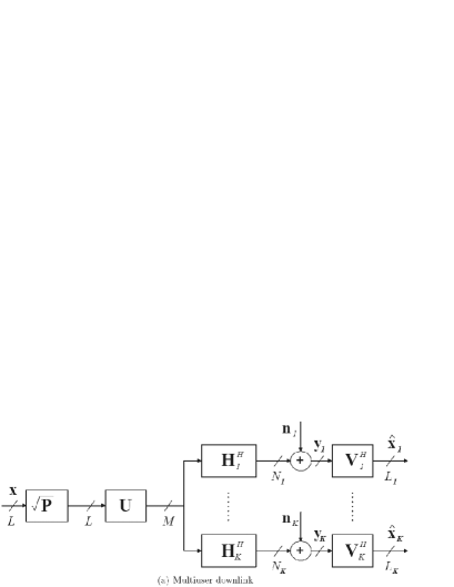
Figure 1: Block Diagram of Multiuser MIMO Downlink

In [13], we showed that the sum mean squared error of the whole system can be written as,

$$SMSE = \sum_{i=1}^{L}E\left[||x_{i}-\hat{x}_{i}||^{2}\right]$$ (3)

$$= L-M+\left(\sigma^{2}+\sigma^{2}_{E}P_{max}\right)tr\left[\mathbf{J}^{-1}\right]$$ (4)

$\mathbf{J}=\mathbf{F}\mathbf{Q}\mathbf{F}^{H}+\left(\sigma^{2}+\sigma^{2}_{E}P_{max}\right)\mathbf{I}_{M}$. $\sigma^{2}_{E}$ denotes the quantization error variance of the feedback model and $\mathbf{Q}$ represents the virtual uplink power allocation matrix. (4) is a nonincreasing function of $\sigma^{2}_{E}$. Our objective is to minimize $\sigma^{2}_{E}$ by designing a backward adaptive differential feedback system.

TABLE I: (Channel Parameters)

Parameter	Value(units)
Carrier Frequency ($\mathbf{f}_{c}$)	2.5 GHz
Channel Sampling Rate ($\mathbf{f}_{s}$)	200 Hz
Frame Duration ($\mathbf{T}_{f_{r}}$)	5 ms

Channel Mobility: The channels are temporally correlated and assumed to follow a modified version of Jakes’ model [14]. Here, channel parameters are selected (as in Table I) to represent typical values for the WiMax standard [1].

Feedback Model: We use two different feedback methods. In the first method, the full channel matrix is quantized and sent back to the base station (BS). The receivers expend 2 bits on the differential quantization of the real and imaginary parts of each scalar channel entry based on minimum Euclidean distance. The BS uses the following channel model:

$$\hskip 7.22743pt\mathbf{H}=\mathbf{\widehat{H}}+\mathbf{\widetilde{H}}$$ (5)

Here $\mathbf{\hat{H}}$ and $\mathbf{\widetilde{H}}$ denote the quantized channel and error in channel feedback respectively. This channel model is used to find the optimal $\mathbf{F}$ through iteration [15]. Also, $\sigma^{2}_{E}=E\left[|h-\hat{h}|^{2}\right]$, $h$ and $\hat{h}$ denote the original and quantized channel entry.

In the second method, the receivers use, as $\mathbf{V}_{k}$, the $L_{k}$ right singular vectors corresponding to the maximum singular values of $\mathbf{H}_{k}$. So, $\mathbf{V}_{k}=\mathbf{B}_{k}(:,1:L_{k})$ Therefore, $\mathbf{F}_{k}=\mathbf{A}_{k}(:,1:L_{k})\times\mathbf{\Sigma}_{k}(:,1:L_{k})$. The receivers perform 2 bits adaptive differential quantization of each real and imaginary scalar entry of $\mathbf{A}_{k}(:,1:L_{k})$ and 2 bit fixed quantization of the entries of $\mathbf{\Sigma}_{k}(:,1:L_{k})$. The BS assumes the following model,

$$\hskip 7.22743pt\mathbf{F}=\mathbf{\widehat{F}}+\mathbf{\widetilde{F}}$$ (6)

Here, $\mathbf{\widehat{F}}$ and $\mathbf{\widetilde{F}}$ represent the quantized effective channel and error in the feedback respectively. Here, $\sigma^{2}_{E}=E\left[|f-\hat{f}\right|^{2}]$. $f$ and $\hat{f}$ denote the scalar entries of $\mathbf{\widehat{F}}$ and $\mathbf{\widetilde{F}}$ respectively.

The linear precoding algorithms of these two feedback models can be found in [15] and  [16] respectively. We do not include those here for brevity.

III Quantization of Channel Entries

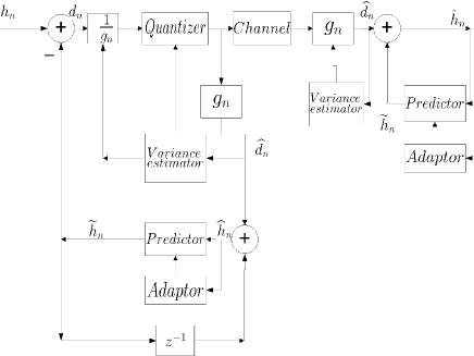
Figure 2: Block Diagram of the adaptive differential quantizer

Stroh [12] proposed the differential quantizer model, shown in Fig. 2, for speech quantization. We use it to perform adaptive differential channel quantization. The left and right sides of the channel block are located at the receiver and base station respectively. A unit variance Gaussian quantizer [17] is used in the quantizer block. Let $h_{n}$ and $\hat{h}_{n}$ represent the original and quantized channel parameter at the $n^{\mathrm{th}}$ instant. $d_{n}$ is the difference between $h_{n}$ and predicted channel $\tilde{h}_{n}$. $g_{n}$ normalizes the variance of the difference signal, i.e., avoids granular noise and overloading. Thus, $g_{n}$ enables the quantizer block to adapt to different speeds. $\hat{d}_{n}=d_{n}+qn_{n}$ where $qn_{n}$ is the quantization noise.

Using the symmetry of the receiver and BS, $\hat{h}_{n}=h_{n}+qn_{n}$ [18, 12]. Here, the adaptor block controls the predictor coefficients and the variance estimator block estimates $g_{n}$. The predictor coefficients and variance estimator parameters depend on $\mathbf{\hat{h}}_{n}$ and $\mathbf{\hat{d}}_{n}$, rather than on $\mathbf{h}_{n}$ and $\mathbf{d}_{n}$. Therefore, unlike the differential feedback model proposed in [10, 9, 11], the BS can reproduce the predictor and variance estimator parameters without the explicit transmission of the coefficients. Since the real and imaginary part are quantized separately, $g_{n}=2\sigma^{2}_{E}$.

III-A Parameter Selection of the adaptive quantizer

III-A1 LLS Based Predictor

Stroh proposed the following LLS based predictor in the speech quantizer [12],

$$\tilde{h}_{n}=\sum^{T}_{j=1}w_{j,n}\hat{h}_{n-j}$$ (7)

Here, $T$ is the predictor order and $\mathbf{w}_{j,n}$ is the $j^{\mathrm{th}}$ weight coefficient at the $n^{\mathrm{th}}$ time instant. The predictor coefficients are computed to minimize the mean squared error

$$\epsilon^{2}=\frac{1}{Lp}\sum^{L_{p}}_{i=1}\left[\hat{h}_{n-i}-\sum^{T}_{j=1}w_{j,n}\hat{h}_{n-i-j}\right]^{2}$$ (8)

Here, $L_{p}$ is the learning period. $\epsilon^{2}$ is the fitting or average prediction error. The weights are calculated through Weiner filtering [19].

TABLE II: (Design Parameters)

Parameter	$\lambda$	$k_{2}$	$k_{1}$	$T$	$L_{P}$
Value	0.98	0.9	1.1	2	100

III-A2 RLS Based Predictor

LLS predictors perform close to ideal Weiner filter predictors in terms of quantization error reduction. However, reducing the steady state error to acceptable levels requires increasing the learning period and an attendant increase of transient time. This motivates us to design a recursive least square based backward predictor [19]. The weights $\mathbf{w}(n)$ are calculated by solving the Weiner-Hopf equation, $\mathbf{\Phi}(n)\mathbf{w}(n)=\mathbf{\psi}(n)$; $\mathbf{w(n)}$ is the $T\times 1$ vector of predictor coefficients, at the $n^{\mathrm{th}}$ time instant. $\mathbf{\Phi(n)}\in\mathcal{R}^{T\times T}$ and $\mathbf{\psi(n)}\in\mathcal{R}^{T\times 1}$ are given by,

$$\mathbf{\Phi(n)} = \lambda\mathbf{\Phi(n-1)}+\mathbf{\hat{h}}(n-1)\mathbf{\hat{h}}^{H}(n-1)$$ (9)

$$\mathbf{\psi(n)} = \lambda\mathbf{\psi(n-1)}+\mathbf{\hat{h}}(n-1)\hat{d}^{H}(n-1)$$ (10)

Here, $\mathbf{\hat{h}}(i)=\left[\hat{h}_{i},\cdots,\hat{h}_{i-T+1}\right]$ and $\lambda$ is the memory factor.

III-A3 RLS Variance Estimators

For the RLS variance estimator, $g_{n}$ is calculated as [19],

$$v_{n} = \sum^{n-1}_{i=1}k_{2}^{n-1-i}\hat{d}^{2}_{i}$$ (11)

$$g_{n} = k_{1}\sqrt{(1-k_{2})\left(k_{2}v_{n-1}+\hat{d}^{2}_{n-1}\right)}.$$ (12)

Here, $k_{1}$ and $k_{2}$ denote the bias compensator and memory factor respectively in RLS variance estimator. Table II lists the parameters of the adaptive differential quantizer. The parameters were chosen via numerical simulations.

IV Quantization of singular vectors

The scalar entries of $\mathbf{A}_{k}(:,1:L_{k})$, the left singular vector matrix of $\mathbf{H}$, can be adaptively differentially quantized using the same model shown in Fig. 2. Note that both the adaptive predictors proposed in the previous section do not assume any particular model of the signal; they try to find the “best” predicted value based on the past observations. However, the quantizer in the proposed adaptive differential feedback model assumes a Gaussian distributed input. Therefore, if we can show the entries of $\mathbf{A}_{k}$ to be approximately Gaussian, the model of Fig. 2 can be readily applied to track $\mathbf{A}_{k}$ [20].

The matrix of singular vectors of a rectangular Gaussian matrix is called a Haar matrix [20].
Lemma 1: If $\mathbf{A}_{k}$ is a $\mathbb{C}^{M\times M}$ Haar matrix, $E\left[|\mathbf{A}_{ij}|^{2}\right]=\frac{1}{M}$ , $1\leq i,j\leq M$.
Proof: See  [20].
Lemma 2: The probability distribution of $\sqrt{M}$ times the Haar matrix $\mathbf{A}_{k}$, approaches the standard complex Gaussian measure as $M\rightarrow\infty$.
Proof: See 4.2.11 of  [20].

In practice, the entries of the Haar matrix approach a Gaussian random variable for small values of $M$. To show this, we set $N_{k}=2$ and choose different numbers of transmit antennas, $M$. We generate $10^{5}$ random Gaussian distributed channels, $\mathbf{H}_{k}\in\mathbb{C}^{M\times N_{k}}$, and find the left singular matrix of $\mathbf{A}_{k}\in\mathbb{C}^{M\times M}$. We randomly pick different entries of $\mathbf{A}_{k}$. After normalizing the samples using Lemma 1, we find the 2 bit codebook of the collected samples using k-means clustering [21]. In Table III we compare the codebook with that of a unit variance 2-bit standard Gaussian quantizer [17].

TABLE III: Codebook of scalar entries of left singular matrix

M = 2	M = 3	M = 4	M = 8	Standard Gaussian
-1.34	-1.40	-1.43	-1.48	-1.51
-0.43	-0.44	-0.45	-0.45	0.45
0.43	0.44	0.45	0.45	0.45
1.34	1.40	1.43	1.48	1.51

In Table III, “$M=2$” stands for the 4 level normalized codebook, based on the scalar entries of the left singular matrix with $2$ transmit antennas. The table shows that even for small number of transmit antennas (e.g., 3), the probability distribution of the normalized scalar entries of the Haar matrix resembles the Gaussian distribution.

The degrees of freedom of the Haar unitary matrix is less than the total number of real and imaginary entries. The minimum number of parameters to represent the Haar matrix can be extracted through Givens’ rotations [4]. An adaptive controller for tracking Givens’ rotated parameters have only been provided for pedestrian velocities [4]. The phases and Givens’ rotated angles are not Gaussian distributed and least squares based predictors are not optimum to track these parameters. Therefore, we stick to our proposed adaptive differential quantization policy. This ensures greater adaptability of our model at the cost of slightly higher feedback overhead.

IV-A Adaptive Differential Quantization of singular value

The distribution of the square of the singular values of a Gaussian channel i.e., the eigenvalues of the Wishart matrix can be found in [22]. We perform fixed 2 bit quantization of the singular values using this distribution and the standard Lloyd-Max quantizer.

In this approach, receivers feed back $\mathbf{\hat{F}}=\mathbf{\hat{H}}\mathbf{\hat{V}}$ to the BS, instead of providing $\mathbf{\hat{H}}$. The dimensionality of $\mathbf{H}$ and $\mathbf{F}$ are $M\times N$ and $M\times L$ respectively. Thus, singular vector quantization saves feedback overhead as long as $L\leq N$.

IV-B Discussion

Sections III and IV show that, since we assumed the channel to be Gaussian and the difference of two correlated Gaussian random variables leads to another Gaussian random variable, the model shown in Fig. 2 provides great flexibility and can hold for different vehicle speeds. To the best of our knowledge, this is the only work in adaptive differential limited feedback literature, which can provide both the following advantages:

1. Unlike the Gauss-Markov models of [10, 9, 11], our model works when the normalized autocorrelation between successive channel samples drops below 0.5.

2. Unlike the feedback model proposed by [4, 5], the controlling parameters of the predictor and variance estimator in our model do not depend on the knowledge of the correlation between two successive channel samples.

V Numerical Results

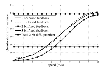
Figure 3: Comparison of of differential feedback with fixed feedback

The channels were generated using the channel model of [14] for each speed. Figure 3 shows the quantization error variance ($\sigma^{2}_{E}=E\left[|h-\hat{h}|^{2}\right]$) of different proposed methods. The quantization error variance plot of a 2-bit and 3-bit unit variance fixed Gaussian quantizer were plotted using the standard values (0.1175 and 0.0345 respectively) [17]. The figure shows that the RLS and LLS predictors perform very similarly in terms of quantization error reduction. The performance of the ideal differential quantizer and predictor is governed by

$$\sigma^{2}_{d_{n}} = \sigma^{2}_{h_{n}}-\psi^{H}\mathbf{\Phi}^{-1}\mathbf{\psi}$$ (13)

$$\sigma^{2}_{qn_{n}} = 0.1175\sigma^{2}_{d_{n}}$$ (14)

Here, (13) follows the minimum error surface of an ideal Weiner filter [19] and (14) follows the quantization error associated with a 2-bit, unit-variance, Gaussian quantizer [17]. The RLS adaptive differential quantizer’s performance becomes inferior as the vehicle velocity exceeds 32 km/h. Using the parameters from Table I, this speed corresponds to a maximum normalized correlation of 0.0255 between two successive channel samples. Therefore, our proposed adaptive differential feedback outperforms fixed quantization as long as the normalized channel autocorrelation remains positive.

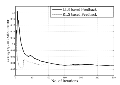
Figure 4: Comparison of the transient time of RLS and LLS based feedback at 21.6 km/hr

Fig. 4 shows that the transient time of RLS adaptive differential feedback is much smaller than the LLS one. The simulation was performed at 21.6 km/hr. The average quantization error was calculated at every iteration. The error variance of the proposed quantizer converges close to its final value within 20 iterations, i.e., 100 ms. Thus, the proposed differential quantizer can adapt itself in real time with reasonable changes in the mobile velocity. Previous works in differential feedback literature have either focused on stationary channels with fixed mobile velocity [9, 10, 11] or non-stationary channels with pedestrian velocity [4, 5]. Our proposed model are suitable for vehicles whose velocity can increase up to 30 km/hr.

Figure 5 shows the average bit error rate (BER) performance of different feedback models at different speeds. We also represent the respective feedback overheads in terms of kilo bit per second (kB/s). We used the system model of Section II, quadrature phase shift keying modulation and the linear transceiver design algorithms of [15] and [16] to simulate the performance of channel and singular-matrix quantization. Here, “adap chan” and “adap eig” denote channel quantization and singular vector quantization respectively. Figure 5 shows that the 2-bit adaptive channel entry feedback outperforms 3-bit fixed feedback and performs very close to the full channel knowledge feedback scenario at 11 km/h . Even at a high speed of 30 km/h (corresponds to a normalized autocorrelation of 0.1 with a $0$ degree arrival angle [23]), the proposed adaptive feedback reduces the BER by a factor of 2, with respect to 2-bit fixed feedback per channel entry.

In Fig. 5, “2 bit adap eig” indicates use of 2 bits to quantize each of the real and imaginary parts of $\mathbf{A}_{k}$ in an adaptive differential manner. Since, we assumed $N=8$ and $L=4$ in our simulation, spending 2 bits per scalar singular matrix entry is equivalent to spending 1 bit per real and imaginary scalar component of the channel. At low speeds like 11 km/h, the singular matrix entry quantizer performs approximately as well as the 2-bit fixed quantizer and reduces the feedback overhead by a factor of 2 for almost same BER. Thus both the adaptive differential feedback methods save 1 bit per real and imaginary entry of the channel matrix at low speed (20 km/h for the channel tracker and 8-9 km/h for the singular matrix tracker). This leads to a saving of $2MNF_{s}$ bits in feedback overhead per second. Using Table I parameters, the proposed systems provide a feedback reduction of $12.8$ kBit/sec.

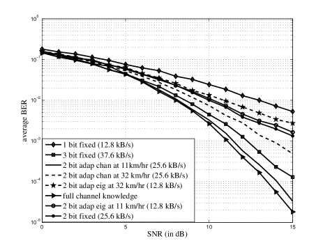
Figure 5: BER and overhead of different feedback methods, $M=4,K=2,N_{1}=4,N_{2}=4,L_{1}=2,L_{2}=2$

VI Conclusions

In this paper, we developed adaptive differential scalar quantization based limited feedback in a time varying multiuser MIMO channel. The key contribution is the development of a differential feedback system that tracks the channel variations without a priori knowledge of the correlation across time, especially the speed of the vehicle.

We proposed two methods of adaptive differential feedback. First, we developed 2-bit adaptive differential quantization of each scalar real and imaginary entry of the MIMO channel. Second, we developed 2-bit adaptive differential quantization of each scalar real and imaginary entry of the singular vectors. Both these methods were shown to significantly reduce the feedback overhead - by as much as 12.8kBit/sec. Our proposed adaptive differential quantizer model was shown to be flexible enough to adapt to different speed of the vehicles.

It is worth emphasizing that one issue not addressed here is adaptive tracking of the channel gains. When different vehicles are located at different distances from the base station, we believe that an adaptive tracking of the channel gain would outperform a fixed channel gain quantizer.

References

- [1] “IEEE standard 802.16e-2005. part 16: Air interface for fixed and mobile broadband wireless access systems-ammendment for physical and medium access control layers for combined fixed and mobile operation in licensed band.,” 2005.
- [2] D. P. Palomar, J. M. Cioffi, and M. A. Lagunas, “Joint tx-rx beamforming design for multicarrier MIMO channels: A unified framework for convex optimization,” IEEE Trans. on Sig. Proc., vol. 51, pp. 2381–2403, Sept. 2003.
- [3] J. C. Haartsen, “Impact of non-reciprocal channel conditions in broadband TDD systems,” in Proc. IEEE PIMRC 2008, Sept. 2008.
- [4] J. C. Roh and B. D. Rao, “An efficient feedback method for MIMO systems with slowly time-varying channels,” in Proc. IEEE WCNC 2004, Mar. 2004.
- [5] A. J. Tenenbaum, R. S. Adve, and Y. Yuk, “Channel prediction and feedback in multiuser broadcast channels,” in Proc. CWIT, 2009.
- [6] N. Jindal, “MIMO broadcast channels with finite-rate feedback,” IEEE Trans. on Comm., vol. 52, pp. 5045–5060, Nov. 2006.
- [7] N. Ravindran and N. Jindal, “Limited feedback-based block diagonalization for the MIMO broadcast channel,” IEEE J. on Selec. Areas in Comm., vol. 26, pp. 1473–1482, Oct. 2008.
- [8] D. J. Love, R. W. Heath, V. K. N. Lau, D. Gesbert, B. D. Rao, and M. Andrews, “An overview of limited feedback in wireless communication systems,” IEEE J. on Selec. Areas in Comm., vol. 26, pp. 2381–2403, Oct. 2008.
- [9] T. Kim, D. J. Love, and B. Clerckx, “A feedback update control scheme for limited feedback multiple antennas systems,” in Proc. IEEE GLOBECOM 2010, Dec. 2010.
- [10] K. Huang, R. W. Heath, and J. G. Andrews, “Limited feedback beamforming over temporally-correlated channels,” IEEE Trans. on Sig. Proc., vol. 57, no. 5, pp. 1959–1975, 2009.
- [11] K. Kim, H. Kim, and D. J. Love, “Utilizing temporal correlation in multiuser MIMO channels,” in Proc. IEEE ASILOMAR 2008, Nov. 2008.
- [12] R. Stroh, Optimum and Adaptive Differential Pulse Colde Modulation, Ph.D. thesis, Polytechnic University, 1970.
- [13] M. N. Islam and R. S. Adve, “Transceiver design using linear precoding in a multiuser mimo system with limited feedback,” IET Journals on Communications, vol. 5, pp. 27–38, 2011.
- [14] Y. R. Zheng and C. Xiao, “Simulation models with correct statistical properties for rayleigh fading channels,” IEEE Transactions on Communications, vol. 51, no. 6, pp. 920–928, 2003.
- [15] A. M. Khachan, A. J. Tenenbaum, and R. S. Adve, “Linear processing for the downlink in multiuser MIMO systems with multiple data streams,” in Proc. IEEE ICC’2006, June 2006, vol. 9, pp. 4113–4118.
- [16] M. N. Islam and R. S. Adve, “Linear transceiver design in a multiuser MIMO sytstem with quantized channel state information,” in Proc. IEEE ICAASP’2010, March 2010.
- [17] S. P. Lloyd, “Least squares quantization in pcm,” IEEE Transactions on Information Theory, vol. 28, pp. 129–137, Mar. 1982.
- [18] J. D. Gibson, “Adaptive prediction in speech differential encoding systems,” Proc. of the IEEE, vol. 68, pp. 488–525, Apr. 1980.
- [19] S. Haykin, Adaptive Filter Theory, Prentice Hall, NJ, 2002.
- [20] F. Hiai & D. Petz, The semicircle law, free random variables, and entropy, American Mathematical Society, RI, 2000.
- [21] Y. Linde, A. Buzo, and R. M. Gray, “An algorithm for vector quantizer design,” IEEE Trans. on Comm., vol. 28, pp. 84–95, Jan. 1980.
- [22] T. Taniguchi, S. Sha, and Y. Karasawa, “Analysis and approximation of statistical distribution of eigenvalues in i.i.d. MIMO channels under rayleigh fading,” IEICE Trans. on Info. Th. and Its Appl., vol. E91-A, pp. 2808–2817, Oct. 2008.
- [23] A. Goldsmith, Wireless Communications, Cambridge Univ. Press, 2005.