The Baldwin effect under multi-peaked fitness landscapes:
Phenotypic fluctuation accelerates evolutionary rate

Abstract

Phenotypic fluctuations and plasticity can generally affect the course of evolution, a process known as the Baldwin effect. Several studies have recast this effect and claimed that phenotypic plasticity accelerates evolutionary rate (the Baldwin expediting effect); however, the validity of this claim is still controversial. In this study, we investigate the evolutionary population dynamics of a quantitative genetic model under a multi-peaked fitness landscape, in order to evaluate the validity of the effect. We provide analytical expressions for the evolutionary rate and average population fitness. Our results indicate that under a multi-peaked fitness landscape, phenotypic fluctuation always accelerates evolutionary rate, but it decreases the average fitness. As an extreme case of the trade-off between the rate of evolution and average fitness, phenotypic fluctuation is shown to accelerate the error catastrophe, in which a population fails to sustain a high-fitness peak. In the context of our findings, we discuss the role of phenotypic plasticity in adaptive evolution.

I Introduction

Phenotypic plasticity is a common process, whereby phenotypic changes occur during an organism’s life cycle. In some cases, phenotypic plasticity can emerge as a response to environmental variation. For example, the desert locust transitions from a solitary to a gregarious phase, depending on population density tawfik1999identification ; gilbert2009ecological . In addition, a phenotype can fluctuate randomly, for example, as a result of the stochasticity of gene expression, exemplified by recent studies in microorganisms spudich1976non ; elowitz2002stochastic ; sato2003relation ; yomo2006responses and animal development west2003developmental ; wernet2006stochastic ; feinberg2010stochastic . Such processes are also interpreted as phenotypic plasticity, and are ubiquitous in nature. Given this, the role of random phenotypic plasticity in adaptive evolution warrants further consideration.

Do phenotypic changes in individuals have any impacts across generations, and thus, influence their evolution? At first glance, phenotypic plasticity does not seem to affect evolutionary processes because only genotypes, rather than phenotypes, are heritable. Non-heritable phenotypes acquired during the life cycle, however, can affect evolution through natural selection because the natural selection acts on acquired phenotypes. This does not mean Lamarckism – heritability of acquired phenotypes, but indicates that genetically determined plasticity, i.e., an ability to change phenotypes, can affect the evolutionary process. This process is referred to as the Baldwin effect, which was first introduced by Baldwin baldwin1896new , and later recast by Simpson simpson1953baldwin . Several studies slatkin1976niche ; moran1992evolutionary ; via1993adaptive ; ancel1999quantitative ; feinberg2010stochastic ; rivoire2011value ; frank2011natural2 have revealed that this effect is advantageous under a fluctuating environment, as phenotypic plasticity can allow organisms to survive sudden environmental changes, and therefore, facilitate adaptation to new environments. However, whether phenotypic plasticity is advantageous throughout evolution, even under fixed environments, is still elusive.

Can phenotypic plasticity accelerate evolutionary rate? This question stems from a recent incarnation of the Baldwin effect known as the ”Baldwin expediting effect” ancel2000undermining . Indeed, the seminal work by Hinton and Nowlan hinton1987learning showed that phenotypic plasticity accelerates evolutionary rate even in fixed environments, although, the validity of these findings is controversial. For example, several subsequent studies have shown that phenotypic plasticity can decelerate evolutionary rate anderson1995learning ; ancel2000undermining ; dopazo2001model , whereas others have claimed that it accelerates evolutionary rate hinton1987learning ; gruau1993adding ; fontanari1990effect ; nolfi1999learning ; price2003role ; borenstein2006effect ; suzuki2007repeated ; paenke2007influence . However, it is important to note that the studiesanderson1995learning ; ancel2000undermining in which it was concluded that phenotypic plasticity leads to a deceleration of evolutionary rate dealt with uni-modal Gaussian fitness landscapes f_Baldwin_1 . Recently, some studies pointed out that, under a multi-peaked fitness, phenotypic plasticity can smoothen fitness valleys, and thus, the escape from a local maximum can be enhanced, leading to the acceleration of evolution frank2011natural ; borenstein2006effect ; asselmeyer1996smoothing ; lande1980genetic . In fact, the acceleration of evolution under a multi-peaked fitness landscape has been confirmed numerically nolfi1999learning ; gruau1993adding ; suzuki2007repeated .

The first analytical result addressing evolution under a multi-peaked fitness landscape in a fixed environment was provided by Borenstein et al. borenstein2006effect , in which they showed that phenotypic plasticity accelerates evolution. Instead of a mutation-selection process, they considered a single random walker on a multi-peaked fitness landscape, to mimic evolutionary population dynamics in genotypic space; therefore, their study did not distinguish between the behaviors of a population and an individual. Thus, in their random walker model the following three points were left unaddressed; first, average population fitness has not been obtained analytically; second, behaviors of the distribution of a population cannot be discussed in their model; and third, the relationship between the acceleration of evolution and average population fitness is unclear. These points should be clarified in order to fully comprehend the role of phenotypic fluctuation (plasticity) in evolutionary population dynamics.

In this study, we investigate evolutionary population dynamics, rather than the single random walker model, under multi-peaked landscapes in a fixed environment, and study the role of phenotypic fluctuation on the evolutionary rate. We provide analytical results for the relationship between phenotypic fluctuation, evolutionary rate, and average population fitness by considering the distribution of genotypes in a population. First, we assess whether a population located at a fitness peak can remain around the peak over generations to maintain high fitness. We show that for both large phenotypic fluctuations and high mutation rates, populations fail to keep descendants near the peak over multiple generations, and therefore, they are unable to maintain a high average fitness. Second, we evaluate the rate at which a population moves between fitness peaks and derive an analytical expression representing the dependency of evolutionary rate on phenotypic fluctuation. The obtained result indicates that phenotypic fluctuation always enhances diffusion in genotypic space, and thus, it accelerates evolution under multi-peaked fitness landscapes.

One consequence of our results is that for a large phenotypic fluctuation, the failure of a population to concentrate near a fitness peak results in a decrease in average fitness. This can be regarded as “error catastrophe.” The concept of error catastrophe refers to the collapse of a population that maintains high fitness because of a high mutation rate eigen1978hypercycle ; eigen1992steps . Our results demonstrate that error catastrophe occurs not only because of a high mutation rate, but also because of large phenotypic fluctuations. Furthermore, our results illustrate an apparent relationship between error catastrophe and the Baldwin effect, in that error catastrophe is explained as an extreme case of a trade-off between an acceleration of evolutionary rate and a decrease in fitness. These findings reveal novel aspects of the role of phenotypic plasticity in evolution.

The organization of this paper is as follows. In Sec. II.1, we explain how phenotypic fluctuation modifies fitness landscapes. In Sec. II.2, we introduce our model of evolutionary population dynamics with phenotypic fluctuation and derive an equation for the time evolution of a population distribution in genotypic space. In Sec III.1 and Sec III.2, we introduce a simple periodic fitness landscape as a multi-peaked fitness landscape. In Sec. III.1, we investigate whether a population can keep its descendants around a peak of fitness, and can sustain high average fitness. In Sec. III.2, we investigate how phenotype fluctuation affects evolutionary rate by using a transformation of the model equation into the Schr$\ddot{\mbox{o}}$dinger equation and adopting WKB approximation. In Sec. III.3, we investigate a quasi-periodic fitness landscape. In Sec. IV, we include concluding remarks.

II Model

II.1 Modulated fitness by phenotypic fluctuation

Let us begin with a discussion of how fitness landscapes are modified by phenotypic fluctuation (also see frank2011natural ; anderson1995learning ; ancel2000undermining ). Note that the phenotypic fluctuation here is sometimes referred to the environmental variance in the context of population genetics and it may also be regarded as an example of phenotypic plasticity. Here, we analyze asexual population dynamics of a single-locus quantitative genetics model. Suppose that an individual organism has two types of a one-dimensional quantitative trait: a heritable trait of genotype $g$ and a non-heritable trait of phenotype $x$. Genotype $g$ is inherited from its parent, whereas phenotype $x$ is given through a genotype-phenotype mapping function $p(x|g;\Sigma)$ with fluctuation magnitude $\Sigma$. Fitness is assigned to each phenotype $x$ and thus is expressed as $F(x)$, given that natural selection acts on phenotypes $x$ rather than genotypes $g$. By calculating the average with respect to $x$, the effective fitness assigned to the genotype $g$ is given as the following equation:

$$f(g)=\int_{\Omega}F(x)p(x|g;\Sigma)dx,$$ (1)

where $\Omega$ is the domain of phenotype value $x$. For simplicity, $p(x|g;\Sigma)$ is assumed to be a Gaussian distribution with mean $g$ and variance $\Sigma$, and $\Omega$ is assumed to be $\Omega=(-\infty,\infty)$;

$$p(x|g;\Sigma)=\frac{1}{\sqrt{2\pi\Sigma}}e^{-\frac{(x-g)^{2}}{2\Sigma}}.$$ (2)

From this simplification, Eq. 1 leads to

$$f(g)=\int_{\Omega}\frac{F(x)}{\sqrt{2\pi\Sigma}}e^{-\frac{(x-g)^{2}}{2\Sigma}}dx.$$ (3)

The above equation reveals that phenotypic fluctuations make a fitness landscape flatter, and its peaks, lower. Examples of such modulation effects are shown in Fig. 1(a) and Fig. 1(b): By flattening the fitness landscape, fitness peak values are decreased, and thus it acts as a cost of phenotypic fluctuation.

II.2 The Discrete Time Model and The Approximated Continuous Time Equation

Once $F(x)$ is given, the effective fitness assigned to individual organisms with genotype $g$ is obtained in Eq. (3). We here consider the evolutionary population dynamics of $N$ individual organisms with non-overlapping generations. Suppose that $N^{t}(g;\Sigma)$ is the frequency distribution of the population at $t$-th generation, and each individual can produce descendants that survive in the next generation at a rate $f(g)/\langle f\rangle$. Here, $\langle\cdot\rangle$ represents an average over the entire population, (e.g., $\langle f\rangle\equiv\int_{\Omega}N^{t}(g;\Sigma)f(g;\Sigma)dg/\int N^{t}(g;\Sigma)dg$). Parental organisms are removed from the population for the next generation. Due to mutations, genotypes of $t+1$-th generation $g^{\prime}$ deviate from the mother’s genotype $g$ as $g^{\prime}=g+\xi$, where $\xi$ is a random number drawn from a Gaussian distribution with a mean zero and variance $D_{g}$. This $D_{g}$ corresponds to mutation rate. This effect of mutations on the distribution $N(g)$ can be written using the mutation operator $M_{g,g^{\prime}}$ as $M_{g,g^{\prime}}[N(g^{\prime})]=\int_{\Omega}N(g^{\prime})\frac{1}{\sqrt{2\pi D_{g}}}e^{-(g-g^{\prime})^{2}/2D_{g}}dg^{\prime}$. By combining both effects of natural selection and mutations, whole evolutionary dynamics is expressed as

$$N^{t+1}(g;\Sigma)=M_{g,g^{\prime}}[\frac{f(g)N^{t}(g)}{\langle f\rangle}]\ .$$ (4)

With an assumption of sufficiently small $D_{g}$, this discrete time equation (4) is approximated by a continuous time equation governed by non-linear Fokker-Planck-like equation: f_Baldwin_2

$$\begin{array}[]{ll}\frac{\partial N(t,g;\Sigma)}{\partial t}&=\frac{f(g;\Sigma)-\langle f\rangle}{\langle f\rangle}N(t,g;\Sigma)+\frac{D_{g}}{2\langle f\rangle}\frac{\partial^{2}}{\partial g^{2}}f(g;\Sigma)N(t,g;\Sigma).\end{array}$$ (5)

In the above equation, $N^{t}(g;\Sigma)$ is replaced by $N(t,g;\Sigma)$, which is a function of continuous time. From this approximation, we can obtain time evolution of a set of moment of $N(t,g;\Sigma)$; for instance

$$\frac{\partial\langle g\rangle}{\partial t}=\frac{\langle gf\rangle-\langle g\rangle\langle f\rangle}{\langle f\rangle}$$ (6)

$$\frac{\partial\langle g^{2}\rangle}{\partial t}=\frac{\langle g^{2}f\rangle-\langle g^{2}\rangle\langle f\rangle}{\langle f\rangle}+D_{g}.$$ (7)

III Results

III.1 Localized-extended transition in a periodic fitness landscape

Here we investigate the model under a simple multi-peaked landscape, namely, a periodic one given as $F(x)=1+\cos\alpha x$. Hence, the effective fitness landscape is expressed as $f(g)=1+\exp(-\alpha^{2}\Sigma/2)\cos\alpha g$ from Eq. (3). First, we investigate whether the population initially located at a peak of fitness can stay around the peak over generations to maintain high fitness. To examine this, we assume that at the initial state $t=0$ all individuals in a population are located at $g=0$, and that the genotype distribution can be approximated by a Gaussian distribution with a mean value $G(t)$ ($=\langle g\rangle$) and variance $V_{g}(t)$ ($=\langle g^{2}\rangle-\langle g\rangle^{2}$) at any generation. This simplification allows us to calculate the time evolution of $N(t,g;\Sigma)$ from Eq. (6) and Eq. (7), resulting in

$$\begin{array}[]{ll}\frac{dG}{dt}&=-\frac{\alpha V_{g}\sin(\alpha G)e^{-\alpha^{2}(\Sigma+V_{g})/2}}{1+e^{-\alpha^{2}(\Sigma+V_{g})/2}\cos\alpha g},\\ \frac{dV_{g}}{dt}&=-\frac{\alpha^{2}V_{g}^{2}\cos(\alpha G)e^{-\alpha^{2}(\Sigma+V_{g})/2}}{1+e^{-\alpha^{2}(\Sigma+V_{g})/2}\cos\alpha G}+D_{g}.\\ \end{array}$$ (8)

The average population fitness is thus obtained as

$$\langle f\rangle=\langle 1+\cos(\alpha g)e^{-\frac{\alpha^{2}\Sigma}{2}}\rangle=1+\cos(\alpha G)e^{-\frac{\alpha^{2}(\Sigma+V_{g})}{2}}.$$ (9)

At the initial state $t=0$, we assume $G(0)=0$ and $V_{g}(0)=0$. Thus, Eq. (8) leads to $dG/dt=0$ (i.e., $G(t)=0$) and

$$\frac{dV_{g}}{dt}=-\frac{\alpha^{2}V_{g}^{2}e^{-\alpha^{2}(\Sigma+V_{g})/2}}{1+e^{-\alpha^{2}(\Sigma+V_{g})/2}}+D_{g}.$$ (10)

The above equation has a fixed point solution when

$$D_{g}<\frac{\alpha^{2}(V_{g}^{*})^{2}e^{-\alpha^{2}(\Sigma+V_{g}^{*})/2}}{1+e^{-\alpha^{2}(\Sigma+V_{g}^{*})/2}},$$ (11)

where $V_{g}^{*}$ gives the minimum of $dV_{g}/dt$ as given by

$$V_{g}^{*}=\frac{2\left(2+W(2e^{-2-\alpha^{2}\Sigma/2})\right)}{\alpha^{2}}.$$ (12)

Here, $W(\cdot)$ is the Lambert W-function defined by the inverse function of $f(W)=We^{W}$. A finite $V_{g}$ at equilibrium indicates that the population is localized around one of the peaks of fitness. When the inequality (11) is not satisfied, $V_{g}$ in Eq. (10) always increases in time, and thus, the variance of $N(t,g;\Sigma)$ goes to infinity, leading to a broad distribution of $N(t,g;\Sigma)$ in genotype space. This qualitative change in the variance $V_{g}$ can be referred to as the localized-extended transition.

Simpler representation of the condition Eq. (11) is obtained by using the approximation $1+\exp[-\frac{\alpha^{2}(\Sigma+V_{g})}{2}]\simeq 1$, which is reasonable around a transition point because variance $V_{g}$ is sufficiently large near the transition point. It yields the condition for a finite variance at equilibrium, namely, the condition for the localized state as follows:

$$D_{g}<\frac{16}{\alpha^{2}}e^{-\alpha^{2}\Sigma/2-2}.$$ (13)

To examine the validity of these arguments, we compare Eq. (11) and Eq. (13) with an individual-based simulation (i.e., direct numerical simulation of Eq. (4)). Figure 2 shows that both the estimates agree rather well with the results from the individual-based simulation.

It should be noted that the Gaussian approximation fails when the population is separated into two subgroups and localized at different peaks of fitness. Because of this failure, the variance of population estimated in the individual-based simulation does not coincide with the approximated value $V_{g}^{eq}$ calculated as a solution of Eq. (10). To remedy this failure, we take account of only one peak with the largest subpopulation, as shown in Appendix B, in which the procedure to determine the boundary between the localized and extended phases from the individual-based simulation is also described.

The average population fitness is theoretically estimated as follows: by solving $dV_{g}/dt=0$ in Eq. (10) by using a quasi-Newton method, we compute $V_{g}^{eq}$, and then the average population fitness is obtained by Eq. (9). The estimated average fitness is shown in Fig. 3. We also estimate the average population fitness by using an alternative approximation method, a harmonic potential approximation, which is given below (see Eq. (20) and also Eq. (38) in Appendix D). These results are shown in Fig. 3, and agree rather well with the results obtained from the individual-based simulation.

Both approximated estimations and results from the individual-based simulation show that in the extended phase, the average population fitness takes a value that is as low as that without selection pressure, namely, $\langle f\rangle=1$. Such a drop in a high fitness value can be interpreted as “error catastrophe”, i.e., the population fails to sustain high fitness due to high mutation rate or large phenotypic fluctuations. In contrast, the population in the localized phase is concentrated around the peak position of the fitness, and thus can sustain a high average fitness.

With the present analysis based on the Gaussian approximation, the population dynamics in relatively short time scale are evaluated to examine whether the population is concentrated around the peak. For a longer time scale, population can jump through the fitness valleys, even in the localized phase as we show in the next section.

III.2 Escape rate analysis in periodic fitness landscape

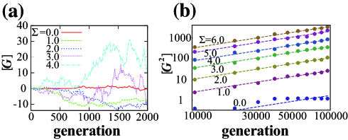
Figure 4: (COLOR ONLINE) Time series of the distribution of population in genotype space. (a) A time series of G (average g over population at each time) obtained by the individual-based simulation. (b) A log-log plot of the time series of $[G^{2}]$, where $[]$ indicates the sample average. In both cases, the average $[\cdot]$ is computed over 100 samples. $[G^{2}]$ for each $\Sigma$ can be fitted to a line with a slope equal to one. This indicates that $G$ performs random walks. In both figures, $N=500$ and $D_{g}=0.3$ are used.

Next we focus on the population dynamics of the localized phase. The population shows diffusion in genetic space, and maintains a high fitness value for longer time scale. Figure 4(a) shows examples of time series of mean genotype value $[G]$ obtained in the individual-based simulations, whereas the time course of its mean square displacement $[G^{2}]$ is plotted in Fig. 4(b). In the figure, $[G^{2}]$ increases in proportion to $t^{1}$, indicating that even in the localized phase the genotype in population performs random walks by jumping across a fitness valley. Through such random walks, a population can search for novel genotypes with a higher fitness value in genotype space without suffering from the error catastrophe. Thus, the diffusion coefficient of this random walk gives a measure for the rate of evolutionary innovations, in other words, evolvability. It should be noted that the deterministic diffusion in genotype space is expected to be observed for infinite population size, although the results from the individual based simulation show stochastic behavior due to finite population size effect.

The diffusion process in genotype space constitutes a sequence of jumps across fitness valleys. As Fig. 1(b) shows, phenotypic fluctuation tends to make fitness valleys shallower, and thus enhances the jump probability from a peak to a neighboring peak. Here, we analytically estimate the jump probability per unit time $\Gamma$ defined as $\int^{\pi/\alpha}_{-\pi/\alpha}N(t,g;\Sigma)dg\sim e^{-2\Gamma t}$, i.e.,

$$\Gamma=-\frac{1}{2t}\log\int^{\pi/\alpha}_{-\pi/\alpha}N(t,g;\Sigma)dg,$$ (14)

with initial condition $N(t=0,g=0;\Sigma)=1$. Note that the jump probability from a peak of fitness to a neighboring peak per unit time is one half of the escape rate in which the jumps to both neighboring peaks have to be considered.

With a separation ansatz $N(t,g;\Sigma)=e^{\lambda t}\phi(g;\Sigma)$, Eq. (5) becomes the following eigenvalue problem:

$$\lambda\phi(g)=\frac{f(g)-\langle f\rangle}{\langle f\rangle}\phi(g)+\frac{D}{\langle f\rangle}\frac{\partial^{2}}{\partial g^{2}}f(g)\phi(g),$$ (15)

where $\phi(g;\Sigma)$ is rewritten as $\phi(g)$ and $D$ is defined as $D=D_{g}/2$. By interpreting $\langle f\rangle$ as an external control parameter $R=\langle f\rangle$, we obtain

$$\Lambda\phi(g)=(f(g)-R)\phi(g)+D\frac{\partial^{2}}{\partial g^{2}}f(g)\phi(g),$$ (16)

where $\Lambda$ is given as

$$\Lambda=R\lambda.$$ (17)

After appropriate transformations of variables f_Baldwin_3 , Eq (16) is transformed into

$$\left(-V(y)+d\frac{\partial^{2}}{\partial y^{2}}\right)\psi=\Lambda\psi,$$ (18)

where

$$V(y)=-\left(f(g(y))-R+\frac{U^{\prime\prime}(y)}{2}-\frac{(U^{\prime}(y))^{2}}{4d}\right).$$ (19)

If we use $t_{sc}=-i\hbar t$ and $m_{sc}=\hbar^{2}/2d$, this agrees with the familiar form of Schr$\ddot{\mbox{o}}$dinger equation.

The Schr$\ddot{\mbox{o}}$dinger form Eq. (18) with WKB approximation simmonds1998first ; landauquantum allows us to estimate the jump probability between a peak of fitness and another peak as an escape rate from a double well potential, assuming that the probability distribution is located only in the left well at $t=0$, as is illustrated in Fig. 5. Details of the derivation are given in Appendix D.

Now, we consider the same fitness landscape in Sec. III.1: $f(g)=1+\chi\cos\alpha g$ and $\chi=\exp(-\alpha^{2}\Sigma/2)$, where $\chi$ decreases as phenotypic fluctuation $\Sigma$ increases. Using quasi equilibrium approximation (see details in Appendix D), the average population fitness $R$ for this landscape can be derived as follows:

$$R=1+\chi-D\frac{\alpha^{2}}{4}\chi-\sqrt{\frac{\alpha^{2}D(1+\chi)\chi}{2}+\frac{\alpha^{4}D^{2}\chi^{2}}{16}}.$$ (20)

This evaluation of average fitness $R$ at the quasi equilibrium agrees rather well with the results from the individual-based simulation, as is shown in Fig. 3 (the thick line represents the evaluation in Eq. (20) ), indicating that the quasi equilibrium approximation is valid.

Using WKB approximation and $R$ estimated above, we can evaluate the jump probability per unit time $\Gamma$ as

$$\begin{array}[]{ll}\Gamma&=\frac{\sqrt{2\alpha^{2}D\chi(1+\chi)}}{R\pi}\exp\left(-\frac{2}{\sqrt{D}}\int_{b}^{\pi/\alpha}\sqrt{\frac{\chi(1-\cos\alpha g)+\Theta(g)}{1+\chi\cos\alpha g}}dg\right),\end{array}$$ (21)

where

$$\begin{array}[]{ll}\Theta(y)&=-\sqrt{\frac{D}{2}(1+\chi)\alpha^{2}\chi+\frac{D^{2}}{16}\alpha^{4}\chi^{2}}\\ &+\frac{D\chi^{2}\alpha^{2}}{8}\frac{\sin^{2}\alpha g}{1+\chi\cos\alpha x}-\frac{\alpha^{2}\chi D}{4}(1-\cos\alpha g)\end{array}$$ (22)

Note that $g=b$ is a point where the integrand becomes zero i.e., $b$ satisfies

$$\chi(1-\cos\alpha b)+\Theta(b)=0$$ (23)

The effective diffusion coefficient $D_{e}$ is given by

$$D_{e}=2\frac{\Gamma}{2}\left(\frac{2\pi}{\alpha}\right)^{2}.$$ (24)

The factor $2$ in the above equation appears since the escape rate from a peak of fitness to the left neighbor peak has to be incorporated, as well as that to the right neighbor peak. Equations (21) and Eq. (24) describe the relation between phenotypic fluctuation $\Sigma$ and evolvability $D_{e}$.

To examine the validity of the estimation of the escape rate $2\Gamma$ in Eq (21), we compare Eq. (21) with that obtained numerically by the individual-based simulation of Eq. (4) (details of the estimation of the escape rate from the individual-based simulation are explained in Appendix C). As shown in Fig. 6, the two agree rather well. These results shown in Fig. 6 indicate that phenotypic fluctuation always accelerates the evolutionary rate, while large phenotype fluctuation decreases the average population fitness, as is shown in Fig. 3. Therefore, the evolvability and fitness values are in a trade-off relationship.

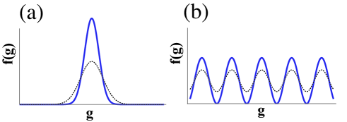
Figure 1: (COLOR ONLINE) Fitness landscapes. (a) A unimodal fitness landscape with (dotted line) and without (line) phenotypic fluctuation. Phenotypic fluctuation modulates an original fitness landscape to that with a lower peak and a wider range. (b) A multi-modal fitness landscape with (line) and without (dotted line) phenotypic fluctuation.

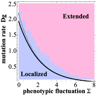
Figure 2: (COLOR ONLINE) A phase diagram for the localized-extended transition. The black line indicates the phase boundary estimated in Eq. (11) and the dotted line indicates the boundary estimated in Eq. (13). The boundary between the blue and red regions is estimated from the individual-based simulation. Details of the estimation are described in Appendix B.

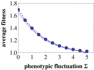
Figure 3: (COLOR ONLINE) Phenotypic fluctuation decreases average population fitness. The fitness are plotted against the phenotype fluctuation $\Sigma$ for $D_{g}=0.2$ and $\alpha=1$. Circles indicate results from the individual-based simulation. The dashed line indicates the approximated value obtained from Eq. (9), where $V_{g}^{eq}$ is calculated numerically from Eq. (10). Thick line indicates the approximated value obtained from a harmonic potential approximation in Eq. (20). Eq. (13) indicates that the error catastrophe occurs as $\Sigma>4.76$ for $\alpha=1.0$, as $\Sigma>2.80$. Because $\alpha$ can be always set as unity by choosing appropriate scaling of $x$, results at $\alpha=1$ is shown.

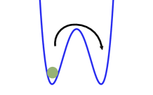
Figure 5: (COLOR ONLINE) A double well potential. The probability is localized at the left well in the initial condition. A jump probability among peaks of fitness can be interpreted as the escape rate from the left well of the double well potential.

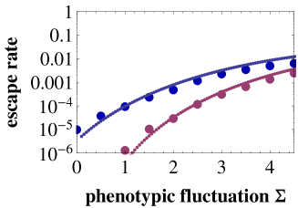
Figure 6: (COLOR ONLINE) Escape rate from a peak of fitness. The escape rate $2\Gamma$ for periodic potential with respect to phenotype fluctuation $\Sigma$. Circles indicate results from the individual-based simulations. Dashed lines indicate the values estimated by using the WKB approximation in Eq. (21). The upper blue line and circles are results for $F(g)=2+\cos\alpha g$ and the lower red line and circles are results for $F(g)=1+\cos\alpha g$. Parameters $N=500$ and $D_{g}=0.2$ are used. Because $\alpha$ can be always set as unity by choosing appropriate scaling of $x$, results at $\alpha=1$ is shown.

III.3 Mixed cosine potential

To demonstrate that our analysis is not limited to the simple periodic potential, we consider the quasi-periodic fitness landscape; $F(x)=A_{1}(1+\cos\alpha_{1}x)+A_{2}(1+\cos\alpha_{2}x)$. From Eq. (1), the effective fitness landscape can be calculated as

$$f(g,\Sigma)=A_{1}(1+e^{-\frac{\alpha_{1}^{2}\Sigma}{2}}\cos\alpha_{1}g)+A_{2}(1+e^{-\frac{\alpha_{2}^{2}\Sigma}{2}}\cos\alpha_{2}g).$$ (25)

An example of the effective fitness $f(g)$ is illustrated in Fig. 7.

Using Gaussian approximation of $N(g;\Sigma)$, we obtain the time evolution of mean value $G$ and variance $V_{g}$ of $N(g;\Sigma)$ as

$$\begin{array}[]{ll}\frac{dG}{dt}&=\\ &-V_{g}\frac{A_{1}\alpha_{1}\sin(\alpha_{1}G)e^{-\alpha_{1}^{2}(\Sigma+V_{g})/2}+A_{2}\alpha_{2}\sin(\alpha_{2}G)e^{-\alpha_{2}^{2}(\Sigma+V_{g})/2}}{A_{1}(1+e^{-\alpha_{1}^{2}(\Sigma+V_{g})/2}\cos\alpha_{1}G)+A_{2}(1+e^{-\alpha_{2}^{2}(\Sigma+V_{g})/2}\cos\alpha_{2}G)}\\ \frac{dV_{g}}{dt}&=\\ &-V_{g}^{2}\frac{A_{1}\alpha_{1}^{2}\cos(\alpha_{1}G)e^{-\alpha_{1}^{2}(\Sigma+V_{g})/2}+A_{2}\alpha_{2}^{2}\cos(\alpha_{2}G)e^{-\alpha_{2}^{2}(\Sigma+V_{g})/2}}{A_{1}(1+e^{-\alpha_{1}^{2}(\Sigma+V_{g})/2}\cos\alpha_{1}G)+A_{2}(1+e^{-\alpha_{2}^{2}(\Sigma+V_{g})/2}\cos\alpha_{2}G)}\\ &+D_{g}\end{array}$$ (26)

Nullcline analysis of Eq. (26) is given in Fig. 8(a) - (c), against the three values of $\Sigma$: for small $\Sigma$ (Fig. 8(a)), a population can be localized at around each local maximum of fitness; for middle value of $\Sigma$ (Fig. 8(b)), a population can be localized only at around a larger local maximum of fitness; for large $\Sigma$ (Fig. 8(c)), all fixed points disappear, and $V_{g}$ diverges, which indicates the extended phase. These results suggest the existence of two transitions: the localized-localized transition and the localized-extended transition.

(i) Localized-localized transition

For the simplicity of discussion, we assume $\alpha_{1}>\alpha_{2}$ in the following argument. Here, we define the localized-localized transition as the transition where a population cannot be localized at around the lowest local maximum of $V(x)$. Thus, we investigate whether a population can be localized around $G_{lm}$, which satisfies

$$\cos(\alpha_{1}G_{lm})=1,$$ (27)

$$\cos(\alpha_{2}G_{lm})=-1.$$ (28)

In other words, we determine the conditions on which $V_{g}$ has finite value for $t\to\infty$ for a population at $G=G_{lm}$ from the following equation:

$$\begin{array}[]{ll}\frac{dV_{g}}{dt}&=\\ &-V_{g}^{2}\frac{A_{1}\alpha_{1}^{2}e^{-\alpha_{1}^{2}(\Sigma+V_{g})/2}-A_{2}\alpha_{2}^{2}e^{-\alpha_{2}^{2}(\Sigma+V_{g})/2}}{A_{1}(1+e^{-\alpha_{1}^{2}(\Sigma+V_{g})/2})+A_{2}(1-e^{-\alpha_{2}^{2}(\Sigma+V_{g})/2})}\\ &+D_{g}.\end{array}$$ (29)

Solving the above equation with an initial condition $V_{g}(0)=0$ by numerical integration, we determine the transition point where $V_{g}$ diverges. In Fig. 9, the blue line shows the localized-localized transition point obtained by the numerical integration.

Intuitive estimation is provided by assuming that the critical value of $V_{g}$ is $\tilde{V_{g}}\sim\left(\frac{\pi}{2\alpha_{1}}\right)^{2}$, which corresponds to the square of the width of a smaller peak. From this assumption, the transition point can be evaluated by

$$\begin{array}[]{ll}D_{g}&\leq(\frac{\pi}{2\alpha_{1}})^{4}\\ &\cdot\frac{A_{1}\alpha_{1}^{2}e^{-\alpha_{1}^{2}(\Sigma+(\frac{\pi}{2\alpha_{1}})^{2})/2}-A_{2}\alpha_{2}^{2}e^{-\alpha_{2}^{2}(\Sigma+(\frac{\pi}{2\alpha_{1}})^{2})/2}}{A_{1}(1+e^{-\alpha_{1}^{2}(\Sigma+(\frac{\pi}{2\alpha_{1}})^{2})/2})+A_{2}(1-e^{-\alpha_{2}^{2}(\Sigma+(\frac{\pi}{2\alpha_{1}})^{2})/2})}.\end{array}$$ (30)

The above estimate agrees well with the results of the numerical integration of Eq. (29) (see Fig. 9).

(ii) Localized-extended transition

To investigate the localized-extended transition, we consider the behaviors of the population distribution located at the global maximum $G=0$. We assume that, near the transition point, $V_{g}$ is large enough to consider $e^{-\alpha_{1}^{2}(\Sigma+V_{g})/2}$ as negligible, but small enough to interpret $e^{-\alpha_{2}^{2}(\Sigma+V_{g})/2}$ as a finite value. From this assumption, Eq. (26) can be rewritten as

$$\begin{array}[]{ll}\frac{dV_{g}}{dt}&=-V_{g}^{2}\frac{A_{2}\alpha_{2}^{2}e^{-\alpha_{2}^{2}(\Sigma+V_{g})/2}}{A_{2}(1+e^{-\alpha_{2}^{2}(\Sigma+V_{g})/2})+A_{1}}+D_{g}.\end{array}$$ (31)

Here, the same procedures to derive Eq. (11) and Eq. (13) are applied. In Fig. 9, we show the estimated localized-extended transition point.

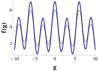
Figure 7: (COLOR ONLINE) A mixed cosine fitness landscape. The landscpe is given by Eq. (25), with (dotted line) and without (line) phenotypic fluctuation. Parameters $A_{1}=2.5,A_{2}=1.0,\alpha_{1}=2.1,\alpha_{2}=1$ are used.

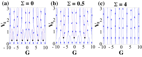
Figure 8: (COLOR ONLINE) Nullcline analysis for Eq. (26). $A_{1}=2.5,A_{2}=1.0,\alpha_{1}=2.1,\alpha_{2}=1$ and $D_{g}=0,1$ are used. The horizontal axis represents $G$, and the vertical axis, $V_{g}$. Black dots indicate stable fixed points. (a) for small $\Sigma$ ($\Sigma=0$), stable fixed points appear around each local maximum of fitness. (b) For $\Sigma=0.5$, some of the stable fixed points vanish, and thus, there are only fixed points around $G=\frac{2\pi}{\alpha_{2}}\times n$, $n=(0,\pm 1,\pm 2,...)$. This indicates that a population is localized only around a peak associated with $\alpha_{2}$. (c) For large $\Sigma$ ($\Sigma=4$), all fixed points vanish. In this case, the population goes to the extended phase.

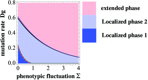
Figure 9: (COLOR ONLINE) A phase diagram of the localized-extended and localized-localized transition for a mixed cosine fitness landscape. Parameters are set as $A_{1}=2.5$, $A_{2}=1.0$, $\alpha_{1}=2.1$, $\alpha_{2}=1$, and $D_{g}=0.1$. The boundary between the localized phases 1 (the left lower phase) and 2 (the middle phase) is estimated by numerical integration of Eq. (29) (gray line) and by Eq. (30) (red dotted line). The boundary between the localized phase 2 and the extended phase (the right upper phase) is estimated by $D=\frac{16}{\alpha_{2}^{2}}\frac{A_{2}}{A_{1}+A_{2}}e^{-\alpha_{2}^{2}\Sigma/2-2}$.

III.4 General Rugged Landscape

Next, we confirm our scenario that phenotypic fluctuation accelerates evolution for a general rugged fitness landscape numerically. Here, we consider a landscape $F(x)=1+\sum_{k}^{M}\frac{\alpha_{k}}{\sum_{j}^{M}\alpha_{j}}\cos\left(\frac{2\pi k}{L}x+\frac{2\pi L}{k}\phi_{k}\right)$, where $\alpha_{k}$ and $\phi_{k}$ are uniform random number ranging over $[0,1]$. Although this landscape is periodic with period $L$, it can be regarded as a random landscape within length $L$. From Eq. (1), the effective fitness landscape can be calculated as

$$f(g,\Sigma)=1+\sum_{k}^{M}\frac{\alpha_{k}}{\sum_{j}^{M}\alpha_{j}}e^{-2\pi^{2}k^{2}\Sigma/L^{2}}\cos\left(\frac{2\pi k}{L}x+\frac{2\pi L}{k}\phi_{k}\right).$$ (32)

Figure 10-(a) shows $f(g,\Sigma)$ for $M=10$, $L=20$. Using this effective fitness landscape, we perform the individual-based simulation. As shown in Fig. 10-(b), the time course of mean square displacement, $[G^{2}]$, of the mean genotypic value $G$ of each generation indicates that diffusion constant in genotype space increases monotonically with $\Sigma$. This demonstrates that phenotypic fluctuation enhances the evolutionary rate (For some case of $F(x)$, the diffusion shows non-monotonic change against $\Sigma$ for small values of $\Sigma$ (data not shown), but for large $\Sigma$, it shows monotonic increase with $\Sigma$).

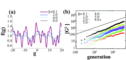
Figure 10: (COLOR ONLINE) (a) A general rugged fitness landscape in Eq. (32) for $M=10$ and $L=20$. Each line represents $f(g,\Sigma)$ for $\Sigma=0.1,2.0,4.0$ and $8.0$. (b) Time course of mean square displacement, $[G^{2}]$, of the mean genotypic value $G$ of each generation for the fitness landscape in (a). The graph is plotted in log-log scale. Average $[\cdot$] is taken over 100 trials. Parameters $N=500$ and $D_{g}=1.0$ are used. Black thick line shows $[G^{2}]=generation$ for reference, while the black dotted line indicates the point where $[G^{2}]=L^{2}=400$; under this line, the landscape can be regarded as a non-periodic random potential.

IV Discussion

In the present study, the evolutionary population dynamics of a simple quantitative genetics model under a multi-peaked fitness landscape is investigated by focusing on the role of phenotypic fluctuation on the evolutionary process. The main results of this study are summarized in the following points (i)-(iv):

(i) The relationship between average fitness and phenotypic fluctuation. Analytical expression is obtained either by Gaussian approximation of a population distribution or by a harmonic potential approximation. By the Gaussian approximation, average fitness is given by Eq. (9) with a solution of ODE Eq. (10) that requires numerical computation, while by the harmonic potential approximation, the average fitness is analytically estimated as Eq. (20) (or Eq. (38)). As is shown in Fig. 3, both approximations agree rather well with the results from the individual-based simulation of evolutionary population dynamics described by Eq. (4) and indicate that average population fitness decreases as the magnitude of phenotypic fluctuation $\Sigma$ increases.

(ii) Error catastrophe due to large phenotypic fluctuation. Because of either a high mutation rate or large phenotypic fluctuation, a population fails to keep its descendants around a peak of fitness, and thus is unable to sustain a high-fitness phenotype. Such a decrease in fitness is known as “error catastrophe.” Although the error catastrophe usually refers to the failure in maintaining the population due to a high mutation rate, our result demonstrates that the error catastrophe can also occur as a result of phenotypic fluctuation. In our model, phenotypic fluctuation always enhances the risk of error catastrophe, whereas an interesting exception to this has been reported in which phenotypic fluctuation can suppress the error catastrophe under a step-like fitness landscape in a high-dimensional genotype space sato2007evolution .

(iii) Dependence of evolutionary rate on the magnitude of phenotypic fluctuation. We provide an analytical expression of the rate at which a population jumps from one peak to another peak in the multi-peaked fitness landscape, which is expressed as the evolutionary rate. The obtained expression Eq. (21) shows that phenotypic plasticity generally enhances evolutionary rate. Such an acceleration has been noted previously gruau1993adding ; frank2011natural ; nolfi1999learning ; borenstein2006effect ; suzuki2007repeated ; however, our results provide the first analytical expression including both the effects of natural selection and mutation. We also confirm numerically that the phenotypic fluctuation accelerates evolution for a general rugged fitness landscape, and thus the present conclusion is not limited to a periodic fitness landscape but is expected to be valid for general landscapes, such as Fig. 10-(a).

Our claim of the acceleration of evolution by phenotypic fluctuation is different from Fisher’s fundamental theorem fisher1930genetical , which claims that genotypic variance is proportional to evolutionary rate. In Fisher’s theorem, the phenotypic plasticity or fluctuations are not considered, and the effect of mutation is also ignored, whereas in our results, genetic variance, phenotypic effect, and the effect of mutation are incorporated. A possible relationship between the phenotypic fluctuation and genotypic variance was also discussed in sato2003relation .

(iv) Phenotypic fluctuation exhibits trade-off relationships with the acceleration of evolution and degradation of fitness. This conclusion is reached by combining the results (i), (ii), and (iii). This trade-off relationship is illustrated by both Fig. 3 and Fig. 6, in which greater phenotypic fluctuation results in a smaller fitness value and a larger evolutionary rate. In addition, the transition to the extended phase (the error catastrophe) for larger phenotypic fluctuation can be interpreted as an extreme situation of this trade-off. It is well established that an increase in mutation rate leads to the same trade-off relationship between the evolutionary rate and degradation of fitness, and that error catastrophe occurs as an extreme case of the trade-off. Our results indicate that phenotypic fluctuation introduces an additional mutation rate, although the origin of the phenotypic fluctuation is essentially different from that of mutation. Note that this “additional mutation rate” effect of phenotypic fluctuation works only in case of multi-peaked fitness landscape, but not in case of a unimodal fitness landscape anderson1995learning ; ancel2000undermining ; dopazo2001model .

Throughout the present study, we interpret random phenotype fluctuation as a kind of phenotypic plasticity (i.e., the phenotypic distribution of a single genotype is independent of environment and fitness (see Eq. (2))). Several previous studies addressing the Baldwin effect also adopted random fluctuation as phenotypic plasticity frank2011natural ; anderson1995learning ; ancel2000undermining ; borenstein2006effect . Our results indicate that even random phenotypic fluctuation accelerates the evolutionary rate under a multi-peaked fitness landscape. Another interpretation of the phenotypic plasticity is that phenotype distribution of a given genotype depends on the fitness landscape, referred to as responsive plasticity hinton1987learning ; fontanari1990effect ; gruau1993adding ; price2003role ; borenstein2006effect ; suzuki2007repeated . The difference between phenotypic fluctuation and responsive plasticity is only in the modulation of a fitness landscape by phenotypic changes, and therefore, the techniques that we adopted in the present study (e.g., the transformation of Fokker-Planck-like equation into the Schr$\ddot{\mbox{o}}$dinger equation, WKB approximation) are applicable after a modulated fitness is obtained; these techniques are generally useful for investigations of evolutionary dynamics PhysRevE.67.061118 ; asselmeyer1997evolutionary ; sato2006distribution ; sato2007evolution .

In our model, we assume that both genotype and phenotype are represented as a one-dimensional continuous value and the mapping between them is straightforward (assumptions often employed in quantitative genetics falconer1981introduction ; anderson1995learning ; ancel2000undermining ). Because such simplicity could miss potential importance of high dimensionality and complexity in real genotype-phenotype mapping, we give brief remarks here. A high dimensional binary genotype model with a simple fitness landscape was adopted in some old studies hinton1987learning ; fontanari1990effect , especially the work by Hinton and Nowlan hinton1987learning demonstrated the validity of Baldwin effect in the model. Recently, relevance of phenotypic fluctuation (noise in developmental process) to mutational robustness has been studied by models with high-dimensional genotype space and with non-trivial genotype-phenotype mapping kaneko2007evolution ; sakata2009funnel ; sakata2011replica . Although these studies did not intend to validate the Baldwin effect, some of their results share a mechanism of the acceleration effect of evolution; their conclusion suggested that smoothening fitness landscape by phenotypic fluctuation prevents from trapping in local maximum of fitness, which is also important for the Baldwin effect. For this reason, it is reasonable to expect that the Baldwin effect is valid even for the case with high dimensional genotype space under a rugged fitness landscape. To confirm this statement, however, further studies are required.

In this paper we study an infinite population model in which population is always genetically polymorphic and there is no fixation event of a single genotype. It will be important for future research to extend our study to include cases with finite populations, in which both the genetic drift and phenotypic fluctuations have to be taken into account seriously.

So far, mounting experimental evidence supports that fitness landscapes in real organisms are multi-peaked fong2005parallel ; korona1994evidence ; hayashi2006experimental . In addition, it has also been shown that stochasticity and random fluctuations in phenotypes are common in living systems spudich1976non ; elowitz2002stochastic ; sato2003relation ; yomo2006responses . In the presence of such fluctuation and multi-peaked fitness landscape, our analytical study has demonstrated the relationship between phenotypic fluctuation and evolutionary rate, as well as the relationship between the Baldwin effect and error catastrophe. Therefore, our findings have broad implications for the study of evolutionary dynamics.

Appendix A Detail of the individual-based simulation

We use an individual-based evolutionary population dynamics model based on an algorithm similar to a genetic algorithm (GA); this simulation is a direct computation of Eq. (4). In this model, each individual in a population has a genotype $g$ and an effective fitness $f(g)$, which is calculated in Eq. (1). We use $F(x)=1+\cos(\alpha x)$ in Sec. III.1 - Sec. III.2 and $F(x)=A_{1}(1+\cos\alpha_{1}x)+A_{2}(1+\cos\alpha_{2}x)$ in Sec. III.3.

In our simulation, total population size is fixed to $N$. At the first generation, each individual has the same genotype $g=0$. At the $t$-th generation, $N$ individuals for the next generation are selected from the current generation; each individual is sampled with probability $f(g)/N\overline{f}$, where $\overline{f}=\sum_{i}^{N}f(g_{i})/N$. Mutations are applied to a selected population in a way in which $g$ of each selected individual is mutated as $g\to g+\xi$. $\xi$ is a random number drawn from a Gaussian distribution $e^{-g^{2}/2D_{g}}/\sqrt{2\pi D_{g}}$, where $D_{g}$ corresponds to the mutation rate. After a selection and mutation procedure, we obtain the $t+1$-th generation. Iterating the procedure, we simulate the population dynamics.

Appendix B Determination of the phase boundary in Fig. 2

To restore the failure of the Gaussian approximation, we take account of only one interval with an integer $n$, $S_{n}=\{g|~{}(2\pi n-\pi)/\alpha<g<(2\pi n+\pi)/\alpha\}$ that has the largest subpopulation. At each time step in the simulation, variance of the population $V_{sim}$ is evaluated by using the subpopulation in $S_{n}$ by the following equation.

$$V_{sim}=\frac{1}{n_{S}}\sum_{i\in S_{n}}(g_{i}-\frac{2\pi n}{\alpha})^{2}$$ (33)

Here, $n_{S}$ indicate the number of individuals in $S_{n}$. We also evaluated $\tilde{V}_{g}^{\ast}$ by truncated Gaussian distribution as

$$\tilde{V_{g}}^{*}=\frac{\int^{\pi/\alpha}_{-\pi/\alpha}g^{2}\exp(-g^{2}/2V_{g}^{*})/\sqrt{2\pi V_{g}^{*}}dg}{\int^{\pi/\alpha}_{-\pi/\alpha}\exp(-g^{2}/2V_{g}^{*})/\sqrt{2\pi V_{g}^{*}}dg},$$ (34)

where $V_{g}^{\ast}$ is calculated by Eq. (12). In Fig. 2, localized (extended) phase is determined by the condition that the time average of $V_{sim}$ is smaller (larger) than $\tilde{V}^{*}$.

Note that the above estimate of $V_{sim}$ using only subpopulation in $S_{n}$ underestimates the variance of the population, because broader distributions of coexisting subpopulations in neighboring peaks are ignored. The agreement between the boundaries by theory and simulation in Fig. 2 could be improved by taking appropriately into account a correction for the estimate of the variance.

Appendix C Details of the evaluation of the escape rate from the individual-based simulation

To evaluate the escape rate of a population from a peak of fitness, we perform the individual-based simulation of Eq.(4) with the following boundary condition: at the initial condition $t=0$, all individuals in a population are located at $g=0$; when an individual escapes from the region $(-\pi/\alpha,\pi/\alpha)$, $g$ of the individual is transformed into $g+M\pi/\alpha$, where $M$ is a sufficiently large integer that the individual never returns to the region $(-\pi/\alpha,\pi/\alpha)$. Note that this transformation does not change the fitness of each individual. Using this boundary condition, we compute time series of the average fraction of a population in the region $(-\pi/\alpha,\pi/\alpha)$ and then estimate the decreasing rate of the average fraction as the escape rate. Here, the average fractions are calculated over 200 trials for $\alpha=1.0,1.2$ and 3000 trials for $\alpha=0.8$. Then the escape rates are calculated as $2\Gamma$ in Eq.(14).

Appendix D WKB approximation

Here, we assume that the population is located only around a peak of fitness. This assumption allows us to suppose that the probability distribution of the Schr$\ddot{\mbox{o}}$dinger equation is only located in the left well at $t=0$, as is illustrated in Fig. 5. Within a time-scale much shorter than that of a jump, we can assume that a population is approximately in an equilibrium state (a quasi equilibrium) in a harmonic potential, which is derived from the Taylor expansion around a minimum of $V(y)$, $y=y^{*}$

$$\begin{array}[]{ll}V(y)&\simeq V(y^{*})+\frac{1}{2}V^{\prime\prime}(y^{*})(y-y^{*})^{2}\\ &=V(y^{*})+\frac{1}{2}\left(-\Xi^{\prime\prime}(y^{*})+\frac{(U^{\prime\prime}(y^{*}))^{2}}{2d}\right)(y-y^{*})^{2},\end{array}$$ (35)

where $\Xi(y)=f(y)-R$. The second term in Eq. (35) is interpreted as $\frac{1}{2}m_{sc}\omega^{2}y^{2}$, and therefore,

$$\frac{1}{2}m_{sc}\omega^{2}=\frac{\hbar^{2}\omega^{2}}{4d}=\frac{1}{2}\left(-\Xi^{\prime\prime}(y^{*})+\frac{(U^{\prime\prime}(y^{*}))^{2}}{2d}\right),$$ (36)

where $\omega$ is the angular frequency of the harmonic potential. The ground energy of the harmonic potential is given by

$$\begin{array}[]{ll}E_{0}&=V_{min}+\frac{\hbar\omega}{2}\\ &=-\left(\Xi(y^{*})+\frac{U^{\prime\prime}(y^{*})}{2}\right)+\sqrt{\frac{d}{2}\left(-\Xi^{\prime\prime}(y^{*})+\frac{(U^{\prime\prime}(y^{*}))^{2}}{2d}\right)}.\end{array}$$ (37)

At the quasi equilibrium, the eigenvalue $E_{0}$ should be zero, yielding

$$R=\hat{f}(y^{*})+\frac{U^{\prime\prime}(y^{*})}{2}-\sqrt{\frac{d}{2}\left(-\Xi^{\prime\prime}(y^{*})+\frac{(U^{\prime\prime}(y^{*}))^{2}}{2d}\right)}$$

$$=f(g^{*})+\frac{D}{4}\frac{\partial^{2}f}{\partial g^{2}}-\sqrt{\left(\frac{Df(g^{*})}{2}|\frac{\partial^{2}f}{\partial g^{2}}(g^{*})|+\frac{D^{2}}{16}(\frac{\partial^{2}f}{\partial g^{2}}(g^{*}))^{2}\right)},$$ (38)

where $\hat{f}(y^{*})=f(g(y^{*}))=f(g^{*})$, $\Xi^{\prime\prime}(y^{*})=\frac{Df(x^{*})}{d}\frac{\partial^{2}f}{\partial g^{2}}|_{g=g^{*}}$ and $U^{\prime\prime}(y^{*})=\frac{D}{2}\frac{\partial^{2}f}{\partial g^{2}}|_{g=g^{*}}$.

The escape rate of the double well potential can be calculated by the difference $\Delta\Lambda$ between the smallest eigenvalue $\Lambda_{0}$ and the second smallest eigenvalue $\Lambda_{1}$ [41, 51, 52]. To derive this difference, the most successful technique is WKB approximation, in which sufficiently small and smooth potential $V(y)$ are assumed. By WKB approximation, the escape rate $\Gamma$ of double well potential can be estimated as [38, 41]

$$\begin{array}[]{ll}\Gamma&=\frac{\Delta\Lambda}{2R}=\frac{\hbar\omega}{R\pi}\exp\left(-\frac{2\sqrt{2m}}{\hbar}\int_{b}^{a}\sqrt{V(y)-E_{0}}dy\right)\\ &=\frac{\hbar\omega}{R\pi}\exp\left(-\frac{2}{\sqrt{d}}\int_{b}^{a}\sqrt{V(y)-E_{0}}dy\right),\end{array}$$ (39)

where $y=b$ is a point in which the integrand becomes zero and $y=a$ is a point in which the integrand becomes a maximum (i.e., the central peak of potential in Fig. 5 ). It should be noted that, from Eq. (17), the time scale of Eq. (5) is R times slower than Eq. (16). The integrand in Eq. (39) can be estimated as

$$\begin{array}[]{ll}\sqrt{V(y)-E_{0}}&=\sqrt{-\left(\Xi(y)+\frac{U^{\prime\prime}(y)}{2}-\frac{(U^{\prime}(y))^{2}}{4d}\right)}\\ &=\sqrt{R-\hat{f}(y)-\left(\frac{U^{\prime\prime}(y)}{2}-\frac{(U^{\prime}(y))^{2}}{4d}\right)}\\ &=\sqrt{f(g^{*})-\hat{f}(y)+\Theta(y)},\end{array}$$ (40)

where

$$\begin{array}[]{ll}\Theta(y)&=-\sqrt{-\frac{Df(g^{*})}{2}\frac{\partial^{2}f(g^{*})}{\partial g^{2}}+\frac{D^{2}}{16}(\frac{\partial^{2}f(g^{*})}{\partial g^{2}})^{2}}\\ &+\frac{D}{8f}(\frac{\partial f(g)}{\partial g})^{2}+\frac{D}{4}(\frac{\partial^{2}f(g^{*})}{\partial g^{2}}-\frac{\partial^{2}f(g)}{\partial g^{2}}).\end{array}$$ (41)

Thus, equation Eq. (39) becomes

$$\begin{array}[]{ll}\Gamma&=\frac{\hbar\omega}{R\pi}\exp\left(-\frac{2}{\sqrt{d}}\int_{b}^{a}\sqrt{f(g(y^{*}))-f(g(y))+\Theta(y)}dy\right)\\ &=\frac{\hbar\omega}{R\pi}\exp\left(-\frac{2}{\sqrt{d}}\int_{g^{*}}^{g_{a}}\sqrt{f(g^{*})-f(g)+\Theta(y)}\frac{dy}{dg}dg\right)\\ &=\frac{\sqrt{2Df(g^{*})|f^{\prime\prime}(g^{*})|}}{R\pi}\exp\left(-\frac{2}{\sqrt{D}}\int_{g^{*}}^{g_{a}}\sqrt{\frac{f(g^{*})-f(g)+\Theta(y(g))}{f(g)}}dg\right).\end{array}$$ (42)

Note that, in the above equation, we use $\hbar\omega=\sqrt{D|f^{\prime\prime}(g^{*})|(2f(g^{*})+D|f^{\prime\prime}(g^{*})|/4)}\simeq\sqrt{2Df(g^{*})|f^{\prime\prime}(g^{*})|}$ from Eq. (36).

References

- [1] A.I. Tawfik, S. Tanaka, A. De Loof, L. Schoofs, G. Baggerman, E. Waelkens, R. Derua, Y. Milner, Y. Yerushalmi, and M.P. Pener. Identification of the gregarization-associated dark-pigmentotropin in locusts through an albino mutant. Proceedings of the National Academy of Sciences, 96(12):7083, 1999.
- [2] S.F. Gilbert and D. Epel. Ecological developmental biology: integrating epigenetics, medicine, and evolution. Sinauer Associates Sunderland, MA, 2009.
- [3] J.L. Spudich, DE Koshland Jr, et al. Non-genetic individuality: chance in the single cell. Nature, 262(5568):467, 1976.
- [4] MB Elowitz, AJ Levine, ED Siggia, and PS Swain. Stochastic gene expression in a single cell. Science (New York, NY), 297(5584):1183, 2002.
- [5] K. Sato, Y. Ito, T. Yomo, and K. Kaneko. On the relation between fluctuation and response in biological systems. Proceedings of the National Academy of Sciences, 100(24):14086, 2003.
- [6] T. Yomo, K. Sato, Y. Ito, and K. Kaneko. Responses of fluctuating biological systems. Biologically Inspired Approaches to Advanced Information Technology, pages 107–112, 2006.
- [7] M.J. West-Eberhard. Developmental plasticity and evolution. Oxford University Press, 2003.
- [8] M.F. Wernet, E.O. Mazzoni, A. Çelik, D.M. Duncan, I. Duncan, and C. Desplan. Stochastic spineless expression creates the retinal mosaic for colour vision. Nature, 440(7081):174–180, 2006.
- [9] A.P. Feinberg and R.A. Irizarry. Stochastic epigenetic variation as a driving force of development, evolutionary adaptation, and disease. Proceedings of the National Academy of Sciences, 107(suppl 1):1757–1764, 2010.
- [10] M.J. Baldwin. A new factor in evolution. The American Naturalist, 30(354):441–451, 1896.
- [11] G.G. Simpson. The baldwin effect. Evolution, 7(2):110–117, 1953.
- [12] M. Slatkin and R. Lande. Niche width in a fluctuating environment-density independent model. American Naturalist, pages 31–55, 1976.
- [13] NA Moran. The evolutionary maintenance of alternative phenotypes. American Naturalist, 139(5):971–989, 1992.
- [14] S. Via. Adaptive phenotypic plasticity: target or by-product of selection in a variable environment? The American Naturalist, 142(2):352–365, 1993.
- [15] L.W. Ancel. A quantitative model of the simpson-baldwin effect. Journal of Theoretical Biology, 196(2):197–209, 1999.
- [16] O. Rivoire and S. Leibler. The value of information for populations in varying environments. Journal of Statistical Physics, 142(6):1124–1166, 2011.
- [17] S.A. Frank. Natural selection. i. variable environments and uncertain returns on investment*. Journal of Evolutionary Biology, 2011.
- [18] L.W. Ancel. Undermining the baldwin expediting effect: Does phenotypic plasticity accelerate evolution? Theoretical Population Biology, 58(4):307–319, 2000.
- [19] G.E. Hinton and S.J. Nowlan. How learning can guide evolution. Complex systems, 1(1):495–502, 1987.
- [20] R.W. Anderson. Learning and evolution: A quantitative genetics approach. Journal of Theoretical Biology, 175(1):89–101, 1995.
- [21] H. Dopazo, MB Gordon, R. Perazzo, and S. Risau-Gusman. A model for the interaction of learning and evolution. Bulletin of Mathematical Biology, 63(1):117–134, 2001.
- [22] F. Gruau and D. Whitley. Adding learning to the cellular development of neural networks: Evolution and the baldwin effect. Evolutionary computation, 1(3):213–233, 1993.
- [23] JF Fontanari and R. Meir. The effect of learning on the evolution of asexual populations. Complex Systems, 4:401–414, 1990.
- [24] S. Nolfi and D. Floreano. Learning and evolution. Autonomous robots, 7(1):89–113, 1999.
- [25] T.D. Price, A. Qvarnström, and D.E. Irwin. The role of phenotypic plasticity in driving genetic evolution. Proceedings of the Royal Society of London. Series B: Biological Sciences, 270(1523):1433–1440, 2003.
- [26] E. Borenstein, I. Meilijson, and E. Ruppin. The effect of phenotypic plasticity on evolution in multipeaked fitness landscapes. Journal of Evolutionary Biology, 19(5):1555–1570, 2006.
- [27] R. Suzuki and T. Arita. Repeated occurrences of the baldwin effect can guide evolution on rugged fitness landscapes. In Artificial Life, 2007. ALIFE’07. IEEE Symposium on, pages 8–14. IEEE, 2007.
- [28] I. Paenke, B. Sendhoff, and T.J. Kawecki. Influence of plasticity and learning on evolution under directional selection. The American Naturalist, 170(2):E47–E58, 2007.
- [29] Paenke et al. [28] investigated a model of evolution with phenotypic plasticity under uni-modal fitness landscape and demonstrated that the phenotypic plasticity can accelerate evolutionary rate under sharper fittness landscape than Gaussian, while it decelerates evolutionary rate under Gaussian uni-modal fitness landscape.
- [30] S.A. Frank. Natural selection. ii. developmental variability and evolutionary rate*. Journal of Evolutionary Biology, 24(11):2310–2320, 2011.
- [31] T. Asselmeyer, W. Ebeling, and H. Rose. Smoothing representation of fitness landscapes–the genotypephenotype map of evolution. BioSystems, 39(1):63–76, 1996.
- [32] R. Lande. Genetic variation and phenotypic evolution during allopatric speciation. American Naturalist, pages 463–479, 1980.
- [33] M. Eigen and P. Schuster. The hypercycle. Naturwissenschaften, 65(1):7–41, 1978.
- [34] M. Eigen and R. Winkler. Steps towards life: A perspective on evolution. Oxford University Press, USA, 1992.
- [35] is used. See [51, 52].
- [36] By adopting variable as and , where , Eq (16) is transformed into Eq.(18).
- [37] J.G. Simmonds and J.E. Mann. A first look at perturbation theory. Dover Pubns, 1998.
- [38] LD Landau and EM Lifshits. Quantum mechanics: non-relativistic theory (1977) New York. Pergamon, 1977.
- [39] K. Sato and K. Kaneko. Evolution equation of phenotype distribution: general formulation and application to error catastrophe. Physical Review E, 75(6):061909, 2007.
- [40] R.A. Fisher. The genetical theory of natural selection. 1930.
- [41] J. Dunkel, W. Ebeling, L. Schimansky-Geier, and P. Hänggi. Kramers problem in evolutionary strategies. Phys. Rev. E, 67:061118, Jun 2003.
- [42] T. Asselmeyer, W. Ebeling, and H. Rosé. Evolutionary strategies of optimization. Physical Review E, 56(1):1171, 1997.
- [43] K. Sato and K. Kaneko. On the distribution of state values of reproducing cells. Physical Biology, 3:74, 2006.
- [44] Douglas Scott Falconer et al. Introduction to quantitative genetics. Number Ed. 2. Longman., 1981.
- [45] K. Kaneko. Evolution of robustness to noise and mutation in gene expression dynamics. PLoS One, 2(5):434, 2007.
- [46] A. Sakata, K. Hukushima, and K. Kaneko. Funnel landscape and mutational robustness as a result of evolution under thermal noise. Physical review letters, 102(14):148101, 2009.
- [47] A. Sakata, K. Hukushima, and K. Kaneko. Replica symmetry breaking in an adiabatic spin-glass model of adaptive evolution. Europhys. Lett., 99:68004, 2012.
- [48] S.S. Fong, A.R. Joyce, and B.Ø. Palsson. Parallel adaptive evolution cultures of escherichia coli lead to convergent growth phenotypes with different gene expression states. Genome research, 15(10):1365–1372, 2005.
- [49] R. Korona, C.H. Nakatsu, L.J. Forney, and R.E. Lenski. Evidence for multiple adaptive peaks from populations of bacteria evolving in a structured habitat. Proceedings of the National Academy of Sciences, 91(19):9037, 1994.
- [50] Y. Hayashi, T. Aita, H. Toyota, Y. Husimi, I. Urabe, and T. Yomo. Experimental rugged fitness landscape in protein sequence space. PLoS One, 1(1):e96, 2006.
- [51] H. Risken. The Fokker-Planck equation: Methods of solution and applications, volume 18. Springer Verlag, 1996.
- [52] N.G. van Kampen. Stochastic processes in physics and chemistry. North holland, 2007.