Symbiotic two-component gap solitons

Abstract

We consider a two-component one-dimensional model of gap solitons (GSs), which is based on two nonlinear Schrödinger equations, coupled by repulsive XPM (cross-phase-modulation) terms, in the absence of the SPM (self-phase-modulation) nonlinearity. The equations include a periodic potential acting on both components, thus giving rise to GSs of the “symbiotic” type, which exist solely due to the repulsive interaction between the two components. The model may be implemented for “holographic solitons” in optics, and in binary bosonic or fermionic gases trapped in the optical lattice. Fundamental symbiotic GSs are constructed, and their stability is investigated, in the first two finite bandgaps of the underlying spectrum. Symmetric solitons are destabilized, including their entire family in the second bandgap, by symmetry-breaking perturbations above a critical value of the total power. Asymmetric solitons of intra-gap and inter-gap types are studied too, with the propagation constants of the two components falling into the same or different bandgaps, respectively. The increase of the asymmetry between the components leads to shrinkage of the stability areas of the GSs. Inter-gap GSs are stable only in a strongly asymmetric form, in which the first-bandgap component is a dominating one. Intra-gap solitons are unstable in the second bandgap. Unstable two-component GSs are transformed into persistent breathers. In addition to systematic numerical considerations, analytical results are obtained by means of an extended (“tailed”) Thomas-Fermi approximation (TFA).

¹Department of Telecommunication Engineering, Mahanakorn University of Technology,
Bangkok 10530, Thailand
²Department of Physical Electronics, School of Electrical Engineering,
Faculty of Engineering, Tel Aviv University, Tel Aviv 69978, Israel
^∗ bluethawatch@mut.ac.th

(190.6135) Spatial solitons; (160.5293) Photonic bandgap materials; (020.1475) Bose-Einstein condensates.

1 Introduction

Studies of solitons in spatially periodic (lattice) potentials have grown into a vast area of research, with profoundly important applications to nonlinear optics, plasmonics, and matter waves in quantum gases, as outlined in recent reviews [1, 2, 3, 4]. In ultracold bosonic and fermionic gases, periodic potentials can be created, in the form of optical lattices, by coherent laser beams illuminating the gas in opposite directions [5, 6, 7]. Effective lattice potentials for optical waves are induced by photonic crystals, which are built as permanent structures by means of various techniques [2, 8, 9], or as laser-induced virtual structures in photorefractive crystals [10]. Parallel to the progress in the experiments, the study of the interplay between the nonlinearity and periodic potentials has been an incentive for the rapid developments of theoretical methods [11, 12]. Both the experimental and theoretical results reveal that solitons can be created in lattice potentials, if they do not exist in the uniform space [this is the case of gap solitons (GSs) supported by the self-defocusing nonlinearity, see original works [13, 14, 15, 16] and reviews [17, 7]], and solitons may be stabilized, if they are unstable without the lattice (multidimensional solitons in the case of self-focusing, as shown in Refs. [18, 19, 20, 21, 22, 23, 24, 25], see also reviews [1, 3, 4]). The stability of GSs has been studied in detail too—chiefly, close to edges of the corresponding bandgaps—in one [27, 28, 29] and two [30] dimensions alike.

An essential extension of the theme is the study of two-component solitons in lattice potentials. In particular, if both the self-phase-modulation and cross-phase-modulation (SPM and XPM) nonlinearities, i.e., intra- and inter-species interactions, are repulsive, one can construct two-component GSs of intra-gap and inter-gap types, with chemical potentials of the components (or propagation constants, in terms of optical media) falling, respectively, into the same or different bandgaps of the underlying linear spectrum [31, 32]. In the case of the attractive SPM, a family of stable semi-gap solitons was found too, with one component residing in the infinite gap, while the other stays in a finite bandgap [32]. The GSs supported by the XPM repulsion dominating over the intrinsic (SPM-mediated) attraction may be regarded as an example of symbiotic solitons. In the free space (without the lattice potential), symbiotic solitons are supported by the XPM attraction between their two components, despite the action of the repulsive SPM in each one [33, 34, 35]. This mechanism may be additionally enhanced by the linear coupling (interconversion) between the components [36]. Another case of the “symbiosis” was reported in Ref. [37], where the action of the lattice potential on a single component was sufficient for the stabilization of two-dimensional (2D) two-component solitons against the collapse, the stabilizing effect of the lattice on the second component being mediated by the XPM interaction. In addition, the attraction between the components, competing with the intrinsic repulsion, may cause spatial splitting between two components of the GS, as for these components, whose effective masses are negative [15], the attractive interaction potential gives rise to a repulsion force [38, 32].

The ultimate form of the model which gives rise to two-component GSs of the symbiotic type is the one with no intra-species nonlinearity, the formation of the GSs being accounted for by the interplay of the repulsion between the components and the lattice potential acting on both of them. In optics, the setting with the XPM-only interactions is known in the form of the “holographic nonlinearity”, which can be induced in photorefractive crystals for a pair of coherent beams with a small angle between their wave vectors, giving rise to single- [39, 40] and double-peak [41] solitons. Both beams are made by splitting a single laser signal, hence the power ratio between them (which is essential for the analysis reported below) can be varied by changing the splitting conditions. The creation of 2D spatial “holographic solitons” in a photorefractive-photovoltaic crystal with the self-focusing nonlinearity was demonstrated in Ref. [42] (such solitons are stable, as the collapse is arrested by the saturation of the self-focusing). To implement the situation considered here, the sign of the nonlinearity may be switched to self-defocusing by the reversal of the bias voltage, and the effective lattice potential may be induced by implanting appropriate dopants, with the concentration periodically modulated in one direction, which will render the setting quasi-one-dimensional.

In binary bosonic gases, a similar setting may be realized by switching off the SPM nonlinearity with the help of the Feshbach resonance, although one may need to apply two different spatially uniform control fields (one magnetic and one optical) to do it simultaneously in both components. On the other hand, the same setting is natural for a mixture of two fermionic components with the repulsive interaction between them, which may represent two states of the same atomic species, with different values of the total atomic spin ($F$). If spins of both components are polarized by an external magnetic field, the SPM nonlinearity will be completely suppressed by the Pauli blockade while the inter-component interaction remains active [6], hence the setting may be described by a pair of Schrödinger equations for the two wave functions, coupled by XPM terms.

The objective of this work is to present basic families of one-dimensional symbiotic GSs, supported solely by the repulsive XPM nonlinearity in the combination with the lattice potential, and analyze their stability, via the computation of eigenvalues for small perturbations and direct simulations of the perturbed evolution. The difference from the previously studied models of symbiotic solitons [31, 32] is that the solitons where created there by the SPM nonlinearity separately in each component, while the XPM interaction determined the interaction between them and a possibility of creating two-component bound states. Here, the two-component GSs may exist solely due to the repulsive XPM interactions between the components.

We conclude that the symmetric solitons, built of equal components, are destabilized by symmetry-breaking perturbations above a certain critical value of the soliton’s power. The analysis is chiefly focused on asymmetric symbiotic GSs, and on breathers into which unstable solitons are transformed. The model is introduced in Section II, which is followed by the analytical approximation presented in Section III. It is an extended (“tailed”) version of the Thomas-Fermi approximation, TFA, which may be applied to other models too. In Section IV, we report systematic numerical results obtained for fundamental solitons of both the intra- and inter-gap types, hosted by the first two finite bandgaps of the system’s spectrum. The most essential findings are summarized in the form of plots showing the change of the GS stability region with the variation of the degree of asymmetry of the two-component symbiotic solitons, which is a new feature exhibited by the present system. In particular, the stability area of intra-gap solitons shrinks with the increase of the asymmetry, while inter-gap solitons may be stable only if the asymmetry is large enough, in favor of the first-bandgap component, and intra-gap solitons in the second bandgap are completely unstable. The paper is concluded by Section V.

2 The model

The model outlined above is represented by the system of XPM-coupled Schrödinger equations for local amplitudes of co-propagating electromagnetic waves in the planar optical waveguide, $u(x,z)$ and $v(x,z)$, where $x$ and $z$ are the transverse coordinate and propagation distance, without the SPM terms, and with the lattice potential of depth $2\varepsilon>0$ acting on both components:

$$i\frac{\partial u}{\partial z}+\frac{1}{2}\frac{\partial^{2}u}{\partial x^{2}}-|v|^{2}u+\varepsilon\cos(2x)u = 0,$$ (1)

$$i\frac{\partial v}{\partial z}+\frac{1}{2}\frac{\partial^{2}v}{\partial x^{2}}-|u|^{2}v+\varepsilon\cos(2x)v = 0.$$ (2)

The variables are scaled so as to make the lattice period equal to $\pi$, and the coefficients in front of the diffraction and XPM terms equal to $1$. In the case of matter waves, $u$ and $v$ are wave functions of the two components, and $z$ is replaced by time $t$. Direct simulations of Eqs. (1) and (2) were performed with the help of the split-step Fourier-transform technique.

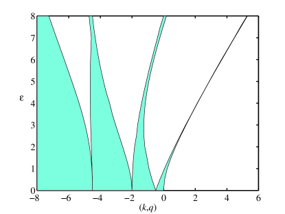
Figure 1: The identical bandgap structures produced by the linearization of Eqs. (4) and (5) for $\varepsilon=6$. Shaded areas are occupied by the Bloch bands, where gap solitons do not exist.

Stationary solutions to Eqs. (1), (2) are looked as

$$u\left(x,z\right)=e^{ikz}U(x),~{}v\left(x,z\right)=e^{iqz}V(x),$$ (3)

where the real propagation constants, $k$ and $q$, are different, in the general case, and real functions $U(x)$ and $V(x)$ obey equations

$$-kU+\frac{1}{2}U^{\prime\prime}-V^{2}U+\varepsilon\cos(2x)U = 0,$$ (4)

$$-qV+\frac{1}{2}V^{\prime\prime}-U^{2}V+\varepsilon\cos(2x)V = 0,$$ (5)

with the prime standing for $d/dx$. Numerical solutions to Eqs. (4) and (5) were obtained by means of the Newton’s method.

Solitons are characterized by the total power,

$$P=\int_{-\infty}^{+\infty}(\left|U\right|^{2}+\left|V\right|^{2})dx\equiv P_{u}+P_{v},$$ (6)

with both $P_{u}$ and $P_{v}$ being dynamical invariants of Eqs. (1), (2), and by the asymmetry ratio,

$$R=\left(P_{u}-P_{v}\right)/\left(P_{u}+P_{v}\right).$$ (7)

The total power and asymmetry may be naturally considered as functions of the propagation constants, $k$ and $q$.

The well-known bandgap spectrum of the linearized version of Eqs. (4), (5) (see, e.g., book [11]) is displayed in Fig. 1, the right edge of the first finite bandgap being

$$k_{\max}\left(\varepsilon=6\right)\approx 3.75.$$ (8)

The location of GSs is identified with respect to bandgaps of the spectrum. In this work, results are reported for composite GSs whose two components belong to the first and second finite bandgaps.

Stability of the stationary solutions can be investigated by means of the linearization against small perturbations [26, 27, 28]. To this end, perturbed solutions of Eqs. (1) and (2) are looked for as

$$u\left(x,z\right) = e^{ikz}\left[U(x)+u_{1}(x)e^{-i\lambda z}+u_{2}^{\ast}(x)e^{i\lambda^{\ast}z}\right],$$

$$v\left(x,z\right) = e^{iqz}\left[V(x)+v_{1}(x)e^{-i\lambda z}+v_{2}^{\ast}(x)e^{i\lambda^{\ast}z}\right],$$ (9)

where $u_{1,2}$ and $v_{1,2}$ are wave functions of infinitesimal perturbations, and $\lambda$ is the respective instability growth rate, which may be complex (the asterisk stands for the complex conjugate). The instability takes place if there is at least one eigenvalue with Im$\left(\lambda\right)>0$. The substitution of ansatz Eqs. (9) into Eqs. (1), (2) and the linearization with respect to the small perturbations leads to the eigenvalue problem based on the following equations:

$$qv_{1}-\frac{1}{2}v_{1}^{\prime\prime}+U^{2}(x)v_{1}+U(x)V(x)\left(u_{1}+u_{2}\right)-\varepsilon\cos(2x)v_{1} = \lambda v_{1},$$ (10)

$$-qv_{2}+\frac{1}{2}v_{2}^{\prime\prime}-U^{2}(x)v_{2}-U(x)V(x)\left(u_{1}+u_{2}\right)+\varepsilon\cos(2x)v_{2} = \lambda v_{2},$$ (11)

$$ku_{1}-\frac{1}{2}u_{1}^{\prime\prime}+V^{2}(x)u_{1}+U(x)V(x)\left(v_{1}+v_{2}\right)-\varepsilon\cos(2x)u_{1} = \lambda u_{1},$$ (12)

$$-ku_{2}+\frac{1}{2}u_{2}^{\prime\prime}-V^{2}(x)u_{2}-U(x)V(x)\left(v_{1}+v_{2}\right)+\varepsilon\cos(2x)u_{2} = \lambda u_{2}.$$ (13)

These equations were solved by means of the fourth-order center-difference numerical scheme.

Results for the shape and stability of GSs of different types are presented below for lattice strength $\varepsilon=6$, which adequately represents the generic case. Note, in particular, that Fig. 1 was plotted for this value of the lattice-potential’s strength.

3 The extended Thomas-Fermi approximation

It is well known that, close to edges of the bandgap, GSs feature an undulating shape, which may be approximated by a Bloch wave function modulated by a slowly varying envelope [13, 15]. On the other hand, deeper inside the bandgap, the GSs are strongly localized (see, e.g., Figs. 4 and 7 below), which suggests to approximate them by means of the variational method based on the Gaussian ansatz [32, 43]. This approximation was quite efficient for the description of GSs in single-component models [43], while for two-component systems it becomes cumbersome [31, 32].

Explicit analytical results for well-localized patterns can be obtained by means of the TFA [5], which, in the simplest case, neglects the kinetic-energy terms, $U^{\prime\prime}$ and $V^{\prime\prime}$, in Eqs. (4), (5). Assuming, for the sake of the definiteness, $q<k$ and also $|k|<\varepsilon$ (the TFA is irrelevant for $|k|>\varepsilon$), the approximation yields the fields inside the inner layer of the solution:

$$\left\{\begin{array}[]{c}U^{2}(x)\\ V^{2}(x)\end{array}\right\}_{\mathrm{inner}}=\left\{\begin{array}[]{c}\varepsilon\cos\left(2x\right)-q\\ \varepsilon\cos\left(2x\right)-k\end{array}\right\},~{}\mathrm{at}~{}~{}|x|<x_{0}\equiv\frac{1}{2}\cos^{-1}\left(\frac{k}{\varepsilon}\right).$$ (14)

Thus, the TFA predicts the core part of the solution in the form of peaks in the two components with the same width, $2x_{0}$, but different heights, $\left\{U^{2},V^{2}\right\}_{\max}=\left\{\varepsilon-q,\varepsilon-k\right\}$. This structure complies with numerically generated examples of asymmetric solitons displayed below in Figs. 7(a,b).

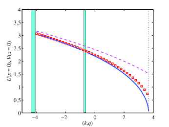
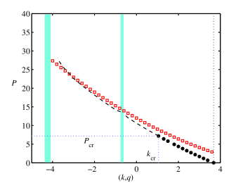
Figure 2: (a) The continuous (blue) curves show the numerically found amplitude of the fundamental symmetric gap solitons (with equal components), versus propagation constant $k=q$, in the first and second bandgaps at $\varepsilon=6.0$. The chain of symbols is the analytical approximation for the same dependence, as produced by the improved TFA in the form of Eq. (16). The dashed curve is the result of the usual TFA, which corresponds to Eq. (16) without the correction (second) terms. (b) Total power $P$ for the same soliton families, whose stable and unstable portions are designated by the bold dotted and dashed lines, respectively. The latter one is destabilized by symmetry-breaking perturbations, while the entire family is stable in the framework of the single-component model. Coordinates of the stability/instability border are given by Eq. (21). The chain of squares shows the analytical dependence produced by the TFA, see Eq. (20).

Further, the expansion of expressions (14) around the soliton’s center ($x=0$), yields

$$\left\{\begin{array}[]{c}U(x)\\ V(x)\end{array}\right\}\approx\left\{\begin{array}[]{c}\sqrt{\varepsilon-q}-\left(\varepsilon/\sqrt{\varepsilon-q}\right)x^{2},\\ \sqrt{\varepsilon-k}-\left(\varepsilon/\sqrt{\varepsilon-k}\right)x^{2}.\end{array}\right\}~{}$$ (15)

The substitution of the second derivatives of the fields at $x=0$, calculated as per Eq. (15), into Eqs. (4), (5) yields a corrected expression for the soliton’s amplitudes:

$$\left\{\begin{array}[]{c}U(x=0)\\ V(x=0)\end{array}\right\}\approx\left\{\begin{array}[]{c}\sqrt{\varepsilon-q}-\varepsilon\left[2\left(\varepsilon-k\right)\sqrt{\varepsilon-q}\right]^{-1},\\ \sqrt{\varepsilon-k}-\varepsilon\left[2\left(\varepsilon-q\right)\sqrt{\varepsilon-k}\right]^{-1},\end{array}\right\}~{}$$ (16)

along with the condition for the applicability of the TFA:

$$\varepsilon\ll\left(\varepsilon-k\right)\left(\varepsilon-q\right).~{}$$ (17)

For the symmetric-GS families in the two first finite bandgaps, the amplitude predicted by the improved TFA in the form of Eq. (16) is displayed, as a function of $k=q$, in Fig. 2(a) and compared to its numerically found counterpart. It is worthy to note that the correction terms in Eq. (16) essentially improve the agreement of the TFA prediction with the numerical findings.

At $|x|>x_{0}$, the TFA gives $V(x)=0$, which is a continuous extension of the respective expression Eq. (14) in the $V$ component, while the continuity of fields $U(x)$ and $U^{\prime}(x)$ makes it necessary to match the respective expression Eq. (14) to “tails”, which, in the lowest approximation, satisfy equation $U^{\prime\prime}=0$. The continuity is provided by the following tail solution:

$$\left\{U^{2}(x)\right\}_{\mathrm{outer}}=\left\{\begin{array}[]{c}\left[\sqrt{k-q}-\sqrt{\left(\varepsilon^{2}-k^{2}\right)/\left(k-q\right)}\left(|x|-x_{0}\right)\right]^{2},{}\\ \mathrm{at}~{}~{}0<|x|-x_{0}<\left(k-q\right)/\sqrt{\varepsilon^{2}-k^{2}};\\ 0,~{}\mathrm{at}~{}~{}|x|-x_{0}>\left(k-q\right)/\sqrt{\varepsilon^{2}-k^{2}}.\end{array}\right\}$$ (18)

The integration of expressions Eq. (14) and Eq. (18) yields the following approximation for the powers of the two components:

$$\left\{\begin{array}[]{c}P_{u}\\ P_{v}\end{array}\right\}_{\mathrm{TFA}}=\left\{\begin{array}[]{c}\sqrt{\varepsilon^{2}-k^{2}}-q\cos^{-1}\left(k/\varepsilon\right)\\ +(2/3)\left(k-q\right)^{2}/\sqrt{\varepsilon^{2}-k^{2}};\\ \sqrt{\varepsilon^{2}-k^{2}}-k\cos^{-1}\left(k/\varepsilon\right).\end{array}\right\}$$ (19)

The substitution of approximation Eqs. (19) into definitions Eq. (6) and Eq. (7) of the total power and asymmetry demonstrates an agreement with numerical results. For instance, the slope of the curve $R(q)$ for the intra-gap GSs at fixed $k$ (see Fig. 8 below) at the symmetry point ($k=q$), as predicted by Eqs. (19) for $\varepsilon=6$ and $k=1$, is $\left(\partial R/\partial q\right)|_{q=k}\approx-0.155,$ while its numerically found counterpart is $\approx-0.160$. Further, the analysis of Eqs. (19) readily demonstrates that the strongly asymmetric solitons may exist up to the limit of $R\rightarrow 1$, which is corroborated by the existence area for the intra-gap solitons shown below in Fig. 11(b).

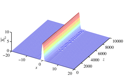
Figure 3: The evolution of a weakly unstable single-component fundamental soliton at $k=-3.7$.

Another corollary of Eqs. (19) is the prediction for the total power for the symmetric solitons,

$$P(k=q)=2\left[\sqrt{\varepsilon^{2}-k^{2}}-k\cos^{-1}\left(k/\varepsilon\right)\right],$$ (20)

which is plotted in Fig. 2(b), along with its numerically found counterpart. Although the TFA does not predict edges of the bandgaps, the overall analytical prediction for $P(k)$ runs quite close to the numerical curve, except for near the right edge, where, indeed condition Eq. (17) does not hold for $\varepsilon=6$ and $k=3.75$, see Eq. (8). Note that this very simple analytical approximation was not derived before in numerous works dealing with single-component GSs.

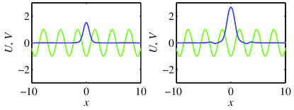
Figure 4: Examples of fundamental symmetric gap solitons found in the first and second bandgaps, for $k=q=2.0$ and $k=q=-2.0$ (left and right panels, respectively). Here and in similar figures below, the background pattern (green sinusoid) represents the underlying periodic potential. Both solitons are stable as solutions of the single-component model, but only the one corresponding to $k=q=2.0$ remains stable in the two-component system, while its counterpart pertaining to $k=q=-2$ is destabilized by symmetry-breaking perturbations.

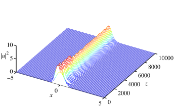
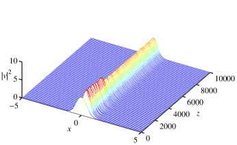
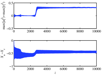
Figure 5: (a) and (b) The spontaneous transformation of an unstable symmetric fundamental soliton for $u$- and $v$-component, in the first bandgap, with $k=q=0$, into a stable asymmetric breather. (c) The top and bottom plots display, respectively, the evolution of the peak-power difference, $\max(\left|u\left(x,z\right)\right|^{2})-\max(\left|u\left(x,z\right)\right|^{2})$, and the separation between centers of the two components, $X_{u}$ and $X_{v}$, which as per Eq. (22).

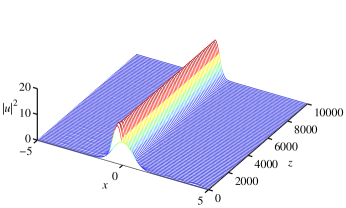
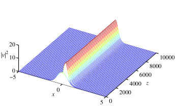
Figure 6: (a,b) The same as in Fig. 5(a,b), but for an unstable soliton in the second bandgap, with $k=q=-3.5$.

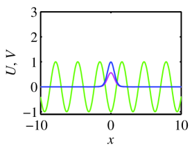
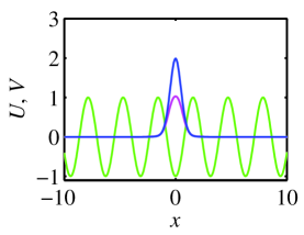
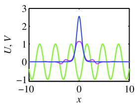
Figure 7: Examples of stable solitons of the intra-gap type found in the first finite bandgap, with fixed asymmetry $R=-0.5$: (a) $k=3$ and $q=3.4601$; (b) $k=1$ and $q=2.843$; (c) $k=-0.5$ and $q=2.5116$. Fields $U(x)$ and $V(x)$, which pertain to propagation constants $k$ and $q$, are shown, respectively, by the magenta (lower) and blue (higher) profiles.

4 Results of the numerical analysis

4.1 Symmetric solitons

Obviously, the shape of symmetric solitons, built of two equal components [with $k=q$ and $U(x)=V(x)$, see Eq. (3)], is identical to that of GSs in the single-component model. However, there is a drastic difference in the stability of the symmetric GSs between the single- and two-component systems. Almost the entire symmetric family is stable against symmetric perturbations, i.e., it is stable in the framework of the single-component equation (in agreement with previously known results [11]), except for a weak oscillatory instability, accounted for by quartets of complex-conjugate eigenvalues, in the form of $\lambda=\pm i\mathrm{Im}\left(\lambda\right)\pm\mathrm{Re}\left(\lambda\right)$ (with two mutually independent signs $\pm$), which appears near the left edge of the second bandgap—namely, at $k<k_{\min}\approx-3.45$. An example the development of the latter instability is displayed below in Fig. 3.

On the other hand, Fig. 2 demonstrates that a considerable part of the family in the first finite bandgap, and the entire family in the second bandgap are unstable against symmetry-breaking perturbations in the two-component system. The boundary separating the stable and unstable subfamilies of the fundamental symmetric GSs in the first finite bandgap corresponds to the power and propagation constants is found at

$$P_{\mathrm{cr}}\approx 7.19,~{}k_{\mathrm{cr}}\approx 1.05,$$ (21)

the symmetric solitons being stable in the intervals of $0<P<7.19$, $1.05<k<k_{\max}\approx 3.75$ [see Eq. (8)]. These results were produced by a numerical solution of Eqs. (10)-(13) (the instability is oscillatory, characterized by complex eigenvalues).

Typical examples of stable and unstable fundamental symmetric GSs, found in the first and second bandgaps (not too close to their edges), are displayed in Fig. 4. Further, direct simulations demonstrate that the evolution transforms the unstable symmetric solitons into persistent localized breathers, as shown in Figs. 5 and 6, in accordance with the fact that the corresponding instability eigenvalues are complex. Although the emerging breather keeps the value of $R=0$, see Eq. (7), the $u$- and $v$- components of the breather generated by the symmetry-breaking instability are no longer mutually identical. This manifestation of the symmetry-breaking instability is illustrated by Fig. 5(c), which displays the evolution of the difference between the peak powers of the two components, and the separation between their centers. The latter is defined as

$$X_{u}-X_{v}\equiv\frac{1}{P_{u}}\int_{-\infty}^{+\infty}|u\left(x,z\right)|^{2}xdx-\frac{1}{P_{v}}\int_{-\infty}^{+\infty}|v\left(x,z\right)|^{2}xdx.$$ (22)

It is relevant to mention that the second finite bandgap also contains a branch of the so-called subfundamental solitons, whose power is smaller than that of the fundamental GSs [44, 45, 46]. These are odd modes, squeezed, essentially, into a single cell of the underlying lattice potential. The subfundamental  solitons are unstable, tending to rearrange themselves into fundamental ones belonging to the first finite bandgap, therefore they are not considered below.

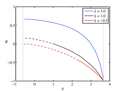
Figure 8: The asymmetry ratio, $R$ [defined as per Eq. (7)], versus propagation constant $q$, at fixed values of $k=3.0$, $1.0$, and $k=-0.5$ (the top, middle, and bottom curves, respectively), for asymmetric fundamental solitons of the intra-gap type. Stable and unstable branches are shown by solid and dashed lines, respectively.

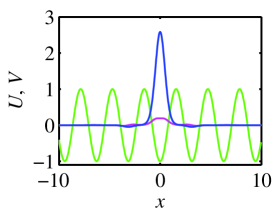
Figure 9: An example of a stable strongly asymmetric soliton with $k=-0.5$ and $q=3.65$. Fields $U(x)$ and $V(x)$, which pertain to propagation constants $k$ and $q$, are shown, respectively, by the magenta (lower) and blue (taller) profiles.

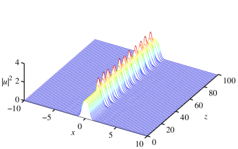
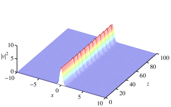
Figure 10: A typical example of the transformation of the unstable asymmetric gap solitons into a breather, for $k=-0.5$ and $q=2.0$.

4.2 Asymmetric solitons of the intra-gap type

As said above, two-component asymmetric fundamental GSs, with different propagation constants, $k\neq q$, may be naturally classified as solitons of the intra- and inter-gap types if $k$ and $q$ belong to the same or different finite bandgaps [31]. In this subsection, we report results for asymmetric intra-gap solitons with both $k$ and $q$ falling into the first finite bandgap, as well as for asymmetric breathers developing from such solitons when they are unstable.

Examples of stable asymmetric GSs of the intra-gap type are displayed in Fig. 7, for a fixed asymmetry ratio, $R=-0.5$, defined as per Eq. (7). The GS family, along with the family of persistent breathers into which unstable solitons are spontaneously transformed, is represented in Fig. 8 by dependences $R(q)$ at different fixed values of the other propagation constant, $k$.

It is possible to explain the fact that all the $R(q)$ curves converge to $R=-1$, as $q$ approaches the right edge of the bandgap in Fig. 8. In this case, the $V$ component turns into the delocalized Bloch wave function with a diverging power, $P_{v}$, that corresponds to $P_{u}/P_{v}\rightarrow 0$ [it is tantamount to $R\rightarrow-1,$ as per Eq. (7)]. An example of a stable GS, close to this limit, with $k=-0.5$, $q=3.65$ and $R=-0.9811$, is shown in Fig. 9. The central core of the $V$-component is described by the TFA, based on Eq. (14), as the corresponding necessary condition (17) holds in this case, while the TFA does not apply to the $U$-component. The presence of undulating tails, which are close to the Bloch functions, rather than the simple approximation (18), which is valid far from the edge of the bandgap, is also visible in Fig. 8.

Those asymmetric intra-gap GSs which form unstable subfamilies in Fig. 8 are destabilized by oscillatory perturbations. The instability transform the solitons into breathers, see a typical example in Fig. 10 [cf. the examples of the destabilization of the symmetric GSs shown in Fig. 5(b,c)]. The emerging breathers keep values of the asymmetry ratio (7) almost identical to those of their parent GSs; for instance, in the case displayed in this figure, the unstable soliton with $R_{\mathrm{initial}}=-0.3617$ evolves into the breather with $R_{\mathrm{final}}=-0.3623$.

It is relevant to stress that the transformation of unstable stationary GSs into the breathers gives rise to little radiation loss of the total power, $P$. On the other hand, in the general case a given unstable gap soliton does not have a stable counterpart with a close value of $P$, hence this unstable soliton cannot transform itself into a slightly excited state of another stable GS. Thus, the breathers represent a distinct species of localized modes.

The most essential results of the stability analysis for the asymmetric solitons of the intra-gap type, and for breathers replacing unstable solitons, are summarized by diagrams in the planes of $\left(k,q\right)$ and $\left(P,R\right)$, which are displayed in Fig. 11. The predictions of the analysis based on the computation of the stability eigenvalues for the stationary solitons, as per Eqs. (10)-(13), always comply with stability tests provided by direct simulations of Eqs. (1) and (2).

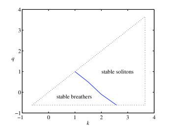
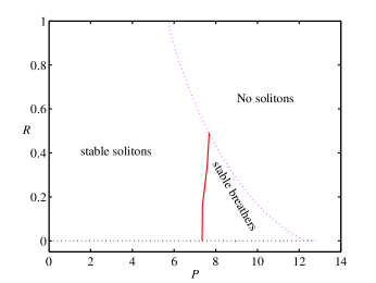
Figure 11: (a) The stability border in the plane of the propagation constants, $\left(k,q\right)$, for asymmetric solitons of the intra-gap type. Only half of the plane is shown, delineated by the dotted triangle, within which wavenumbers $k$ and $q$ belong to the first finite bandgap, as the other half is a mirror image of the displayed one. (b) The same in the plane of the total power and asymmetry ratio, $\left(P,R\right)$, defined as per Eqs. (6) and (7). Localized modes do not exist above the right boundary of the stability regions in panel (b). The diagram at $R<0$ is a mirror image of the one displayed here for $R>0$.

As mentioned above, the instability of a part of the branch of the symmetric solitons along the line of $R=0$ in Fig. 11(b) implies that the symmetry-breaking perturbations destabilize the symmetric solitons in the first finite bandgap at $P>P_{\mathrm{cr}}$, see Eq. (21), while their counterparts are stable in the single-component system. Another clear conclusion is that the stability region gradually shrinks with the increase of the asymmetry.

4.3 Solitons of the inter-gap type

All the GSs of the inter-gap type, with two propagation constants belonging to the two different finite bandgaps, are naturally asymmetric, even if their components have equal powers. Examples of stable and unstable inter-gap solitons are displayed in Figs. 12 and 13, respectively. A noteworthy feature exhibited by these examples is a split-peak structure of the component belonging to the second finite bandgap.

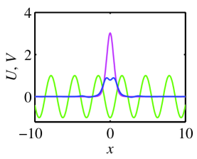
Figure 12: An example of a stable inter-gap soliton, for $k=3$ and $q=-1.65$. The single-peak and split-peak profiles, $U(x)$ and $V(x)$, represent, respectively, the components in the first and second finite bandgaps.

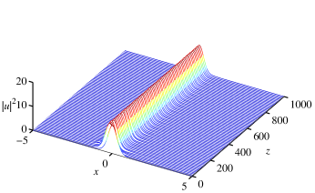
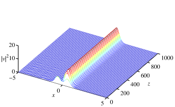
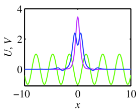
Figure 13: A typical example of the transformation of an unstable intergap soliton into a stable breather, at $k=0$ and $q=-2$. (a,b) The evolution of $|u|^{2}$ and $|v|^{2}$. (c) The initial profiles of $U(x)$ and $V(x)$ (single-peak and split-peak shapes, respectively).

The asymmetry measure, $R(q)$, for families of the inter-gap solitons is plotted in Fig. 14(a) versus the propagation constant $q$ in the second bandgap, at fixed values of $k$ (the propagation constant in the first bandgap). The stability of the respective GS families is also shown in Fig. 14.

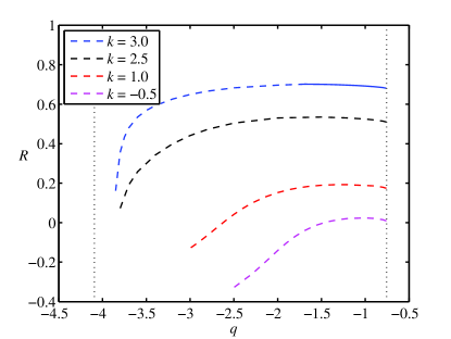
Figure 14: Asymmetry ratio $R$ for the inter-gap solitons versus propagation constant $q$ in the second finite bandgap, at fixed values $k=3.0$, $2.5$, $1.0$, and $-0.5$ (from the top to the bottom) of wavenumber $k$ in the first bandgap. Solid and dashed lines designate stable stationary solitons and breathers, respectively.

The (in)stability of the inter-gap solitons is summarized by the diagrams in the planes of $\left(k,q\right)$ and $\left(P,R\right)$ presented in Fig. 15, cf. similar diagrams for intra-gap solitons shown above in Fig. 11. As well as in that case, unstable inter-gap solitons are spontaneously replaced by robust localized breathers. The spontaneous transformation increases the initial degree of the asymmetry: For instance, an unstable inter-gap soliton with $R=0.019$ is converted into a breather with $R=0.028$.

In the present case too, the existence region of stable modes shrinks with the increase of the asymmetry; note also that the stationary inter-gap solitons may be stable solely at sufficiently large values of the asymmetry, $R\geq R_{\min}\approx 0.5$. The asymmetric shape of the stability diagram in Fig. 15(b) with respect to $R>0$ and $R<0$ [unlike the symmetry of the diagram for the intra-gap solitons implied in Fig. 11(b)] is explained by the fact that, in definition (7), $R>0$ implies that the dominant component resides in the first finite bandgap, where it is more robust than in the second bandgap.

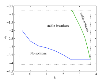
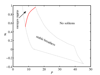
Figure 15: The same as in Fig. 11, but for inter-gap solitons. In (a), the dotted rectangle delineates the region occupied by wavenumbers $k$ and $q$ belonging to the first and second finite bandgaps, respectively.

Finally, out additional analysis has demonstrated that all the stationary GSs—not only the symmetric ones [see Fig. 2], but also all the asymmetric solitons of the intra-gap type—are completely unstable in the second finite bandgap. They too tend to spontaneously rearrange themselves into breathers, which is not shown here in detail.

5 Conclusion

We have introduced the model of symbiotic two-component GSs (gap solitons), based on two nonlinear Schrödinger equations coupled by the repulsive XPM terms and including the lattice potential acting on both components, in the absence of the SPM nonlinearity. The model has a realization in optics, in terms of “holographic solitons” in photonic crystals, and as a model of binary quantum gases (in particular, a fully polarized fermionic one) loaded into the optical-lattice potential. Families of fundamental asymmetric GSs have been constructed in the two lowest finite bandgaps, including the modes of both the intra-gap and inter-gap types, i.e., those with the propagation constants of the two components belonging to the same or different bandgaps, respectively. The existence and stability regions of the symbiotic GSs and breathers, into which unstable solitons are transformed, have been identified. A noteworthy finding is that symmetry-breaking perturbations destabilize the symmetric GSs in the first finite bandgap, if their total power exceeds the critical value given by Eq. (21), along with all the symmetric solitons in the second bandgaps. It was demonstrated too that the stability area for the intra-gap GSs shrinks with the increase of the asymmetry ratio, $R$. On the other hand, inter-gap GSs may be stable only for sufficiently large ratio, $R>0.5$. The intra-gap solitons are completely unstable in the second bandgap. Some features of the GS families were explained by means of the extended TFA (Thomas-Fermi approximation), augmented by the tails attached to the taller component, in the case of asymmetric solitons.

A natural extension of the analysis may deal with 2D symbiotic gap solitons, supported by the square- or radial-lattice potentials. In that case, it may be interesting to consider two-component solitary vortices too.

References

- [1] B. A. Malomed, D. Mihalache, F. Wise, and L. Torner, “Spatiotemporal optical solitons,” J. Opt. B: Quant. Semicl. Opt. 7, R53–R72 (2005).
- [2] F. Lederer, G. I. Stegeman, D. N. Christodoulides, G. Assanto, M. Segev, and Y. Silberberg, “Discrete Solitons in Optics,” Phys. Rep. 463, 1 (2008).
- [3] Y. V. Kartashov, V. A. Vysloukh, and L. Torner, “Soliton shape and mobility control in optical lattices,” Progr. Opt. 52, 63–148 (2009).
- [4] Y. V. Kartashov, B. A. Malomed, and L. Torner, “Solitons in nonlinear lattice,” Rev. Mod. Phys. 83, 247–306 (2011).
- [5] L. Pitaevskii and S. Stringari, Bose-Einstein Condensate (Clarendon Press: Oxford, 2003).
- [6] H. T. C. Stoof, K. B. Gubbels, and D. B. M. Dickerscheid, Ultracold Quantum Fields (Springer: Dordrecht, 2009).
- [7] O. Morsch and M. Oberthaler, “Dynamics of Bose-Einstein condensates in optical lattices,” Rev. Mod. Phys. 78, 179–215 (2006).
- [8] J. D. Joannopoulos, S. G. Johnson, J. N. Winn, and R. D. Meade, Photonic Crystals: Molding the Flow of Light (Princeton University Press: Princeton, 2008).
- [9] A. Szameit, D. Blömer, J. Burghoff, T. Schreiber, T. Pertsch, S. Nolte, and A. Tünnermann, 2005, “Discrete nonlinear localization in femtosecond laser written waveguides in fused silica,” Opt. Express 13, 10552–10557 (2005).
- [10] N. K. Efremidis, S. Sears, D. N. Christodoulides, J. W. Fleischer, and M. Segev, “Discrete solitons in photorefractive optically induced photonic lattices,” Phys. Rev. E 66, 046602 (2002).
- [11] J. Yang, Nonlinear Waves in Integrable and Nonintegrable Systems (SIAM: Philadelphia, 2010).
- [12] D. E. Pelinovsky, Localization in Periodic Potentials (Cambridge University Press: Cambridge, UK, 2011).
- [13] B. B. Baizakov, V. V. Konotop, and M. Salerno, “Regular spatial structures in arrays of Bose–Einstein condensates induced by modulational instability,” J. Phys. B: At. Mol. Opt. Phys. 35, 5105–5119 (2002).
- [14] P. J. Y. Louis, E. A. Ostrovskaya, C. M. Savage, and Y. S. Kivshar, “Bose-Einstein condensates in optical lattices: Band-gap structure and solitons,” Phys. Rev. A 67, 013602 (2003).
- [15] H. Sakaguchi and B. A. Malomed, “Dynamics of positive- and negative-mass solitons in optical lattices and inverted traps,” J. Phys. B 37, 1443–1459 (2004).
- [16] B. Baizakov, B. A. Malomed, and M. Salerno, ”Matter-wave solitons in radially periodic potentials,” Phys. Rev. E 74, 066615 (2006).
- [17] V. A. Brazhnyi and V. V. Konotop, “Theory of nonlinear matter waves in optical lattices,” Mod. Phys. Lett. B 18, 627–651 (2004).
- [18] B. B. Baizakov, B. A. Malomed and M. Salerno, “Multidimensional solitons in periodic potentials,” Europhys. Lett. 63, 642–648 (2003).
- [19] J. Yang, and Z. H. Musslimani, “Fundamental and vortex solitons in a two-dimensional optical lattice,” Opt. Lett. 28, 2094–2096 (2003).
- [20] Z. H. Musslimani and J. Yang, “Self-trapping of light in a two-dimensional photonic lattice,” J. Opt. Soc. Am. B 21, 973–981 (2004).
- [21] B. B. Baizakov, B. A. Malomed and M. Salerno, “Multidimensional solitons in a low-dimensional periodic potential,” Phys. Rev. A 70, 053613 (2004).
- [22] D. Mihalache, D. Mazilu, F. Lederer, Y. V. Kartashov, L.-C. Crasovan, and L. Torner, “Stable three-dimensional spatiotemporal solitons in a two-dimensional photonic lattice,” Phys. Rev. E 70, 055603(R) (2004).
- [23] B. B. Baizakov, B. A. Malomed, and M. Salerno, “Multidimensional semi-gap solitons in a periodic potential,” Eur. Phys. J. 38, 367–374 (2006).
- [24] B. Baizakov, B. A. Malomed, and M. Salerno, “Matter-wave solitons in radially periodic potentials,” Phys. Rev. E 74, 066615 (2006).
- [25] T. Mayteevarunyoo, B. A. Malomed, B. B. Baizakov, and M. Salerno, “Matter-wave vortices and solitons in anisotropic optical lattices,” Physica D 238, 1439–1448 (2009).
- [26] K. M. Hilligsoe, M. K. Oberthaler, and K. P. Marzlin, “Stability of gap solitons in a Bose-Einstein condensate,” Phys. Rev. A 66, 063605 (2002).
- [27] D. E. Pelinovsky, A. A. Sukhorukov, and Y. S. Kivshar, “Bifurcations and stability of gap solitons in periodic potentials,” Phys. Rev. E 70, 036618 (2004).
- [28] G. Hwanga, T. R. Akylas, and J. Yang, “Gap solitons and their linear stability in one-dimensional periodic media,” Physica D 240, 1055–1068 (2011).
- [29] J. Cuevas, B. A. Malomed, P. G. Kevrekidis, and D. J. Frantzeskakis, “Solitons in quasi-one-dimensional Bose-Einstein condensates with competing dipolar and local interactions,” Phys. Rev. A 79, 053608 (2009).
- [30] Z. Shi, J. Wang, Z. Chen, and J. Yang, “Linear instability of two-dimensional low-amplitude gap solitons near band edges in periodic media,” Phys. Rev. A 78, 063812 (2008).
- [31] A. Gubeskys, B. A. Malomed, and I. M. Merhasin, “Two-component gap solitons in two- and one-dimensional Bose-Einstein condensate,” Phys. Rev. A 73, 023607 (2006).
- [32] S. K. Adhikari and B. A. Malomed, “Symbiotic gap and semigap solitons in Bose-Einstein condensates,” Phys. Rev. A 77, 023607 (2008).
- [33] V. M. Pérez-García and J. B. Beitia, “Symbiotic solitons in heteronuclear multicomponent Bose-Einstein condensates,” Phys. Rev. A 72, 033620 (2005).
- [34] S. K. Adhikari, “ Bright solitons in coupled defocusing NLS equation supported by coupling: Application to Bose-Einstein condensation,” Phys. Lett. A 346, 179–185 (2005).
- [35] S. K. Adhikari, “ Fermionic bright soliton in a boson-fermion mixture,” Phys. Rev. A 72, 053608 (2005).
- [36] S. K. Adhikari and B. A. Malomed, “Two-component gap solitons with linear interconversion,” Phys. Rev. A 79, 015602 (2009).
- [37] O. V. Borovkova, B. A. Malomed and Y. V. Kartashov, “Two-dimensional vector solitons stabilized by a linear or nonlinear lattice acting in one component,” EPL 92, 64001 (2010).
- [38] M. Matuszewski, B. A. Malomed, and M. Trippenbach, “Competition between attractive and repulsive interactions in two-component Bose-Einstein condensates trapped in an optical lattice,” Phys. Rev. A 76, 043826 (2007).
- [39] O. Cohen, T. Carmon, M. Segev, and S. Odoulov, “Holographic solitons,” Opt. Lett. 27, 2031–2033 (2002).
- [40] O. Cohen, M. M. Murnane, H. C. Kapteyn, and M. Segev, “Cross-phase-modulation nonlinearities and holographic solitons in periodically poled photovoltaic photorefractives,” Opt. Lett. 31, 954–956 (2006).
- [41] J. R. Salgueiro, A. A. Sukhorukov, and Y. S. Kivshar, “Spatial optical solitons supported by mutual focusing,” Opt. Lett. 28, 1457–1459 (2003).
- [42] J. Liu, S. Liu, G. Zhang, and C. Wang, “Observation of two-dimensional holographic photovoltaic bright solitons in a photorefractive-photovoltaic crystal,” Appl. Phys. Lett. 91, 111113 (2007).
- [43] S. Adhikari and B. A. Malomed, “Gap solitons in a model of a superfluid fermion gas in optical lattices,” Physica D 238, 1402–1412 (2009).
- [44] N. K. Efremidis and D. N. Christodoulides, “Lattice solitons in Bose-Einstein condensates,” Phys. Rev. A 67, 063608 (2003).
- [45] T. Mayteevarunyoo and B. A. Malomed, “Stability limits for gap solitons in a Bose-Einstein condensate trapped in a time-modulated optical lattice,” Phys. Rev. A 74, 033616 (2006).
- [46] J. Cuevas, B. A. Malomed, P. G. Kevrekidis, and D. J. Frantzeskakis, “Solitons in quasi-one-dimensional Bose-Einstein condensates with competing dipolar and local interactions,” Phys. Rev. A 79, 053608 (2009).