Towards the KPP–problem and ${\bf{log\,t}}$–front
shift for higher-order nonlinear PDEs I.
Bi-harmonic and other parabolic equations

Abstract.

The seminal paper by Kolmogorov, Petrovskii, and Piskunov of 1937 [45] on the travelling wave propagation in the reaction-diffusion equation

(0.1) $$u_{t}=u_{xx}+u(1-u)\quad\mbox{in}\quad\mathbb{R}\times\mathbb{R}_{+},\quad u_{0}(x)=H(-x)\equiv\{1\,\,\mbox{for}\,\,x<0;\,\,\,0\,\,\mbox{for}\,\,x\geq 0\}$$

(here $H(\cdot)$ is the Heaviside function), opened a new era in general theory of nonlinear PDEs and various applications. This paper became an encyclopedia of deep mathematical techniques and tools for nonlinear parabolic equations, which, in last seventy years, were further developed in hundreds of papers and in dozens of monographs.

The KPP paper established the fundamental fact that, in (0.1), there occurs a travelling wave $f(x-\lambda_{0}t)$, with the minimal speed $\lambda_{0}=2$, and, in the moving frame with the front shift $x_{f}(t)$ ($u(x_{f}(t),t)\equiv\frac{1}{2}$), there is uniform convergence $u(x_{f}(t)+y,t)\to f(y)$ as $t\to+\infty$, where $x_{f}(t)=2t(1+o(1))$. In 1983, by a probabilistic approach, Bramson [4] proved that there exists an unbounded $\log t$-shift of the wave front in the PDE problem (0.1) and $x_{f}(t)=2t-\frac{3}{2}\,\log t(1+o(1))$ as $t\to+\infty$.

Our goal is to reveal some aspects of KPP-type problems for higher-order semilinear parabolic PDEs, including the bi-harmonic equation and the tri–harmonic one

$$u_{t}=-u_{xxxx}+u(1-u)\quad\mbox{and}\quad u_{t}=u_{xxxxxx}+u(1-u),$$

and other poly-harmonic PDEs up to tenth order. Two main questions to study are:

(i) existence of travelling waves via any analytical/numerical methods, and

(ii) a formal derivation of the $\log t$-shifting of moving fronts.

1. Introduction: the classic KPP–problem, known remarkable results, and extended PDE models

1.1. The classic KPP–problem of 1937: convergence to TWs

In the seminal Kolmogorov–Petrovskii–Piskunov (KPP) problem of 1937 [45]

(1.1) $$u_{t}=u_{xx}+u(1-u)\quad\mbox{in}\quad\mathbb{R}\times\mathbb{R}_{+},\quad u(x,0)=u_{0}(x)\,\,\,\mbox{in\,\, $\mathbb{R}$},$$

with the step (Heaviside) initial function

(1.2) $$u_{0}(x)=H(-x)\equiv\left\{\begin{matrix}1,\quad x<0;\\ 0,\quad x\geq 0,\end{matrix}\right.$$

the solution was proved to converge to the so-called minimal travelling wave (TW) corresponding to

(1.3) $$\mbox{the minimal speed of TW propagation}:\quad\lambda_{0}=2.$$

Namely, looking for a TW profile $f(y)$ for an arbitrary speed $\lambda>0$ yields

(1.4) $$\left\{\begin{matrix}u_{*}(x,t)=f(y),\,\,y=x-\lambda t,\,\,\,\,\mbox{where $f$ solves the ODE problem}\vskip 3.0pt plus 1.0pt minus 1.0pt\vskip 3.0pt plus 1.0pt minus 1.0pt\vskip 3.0pt plus 1.0pt minus 1.0pt\\ -\lambda f^{\prime}=f^{\prime\prime}+f(1-f),\,\,y\in\mathbb{R};\quad f(-\infty)=1,\,\,f(+\infty)=0.\qquad\end{matrix}\right.$$

This 2nd-order ODE, on the phase-plane $\{f,f^{\prime}\}$, by setting $f^{\prime}=P(f)$, reduces its order:

(1.5) $$\textstyle{\frac{{\mathrm{d}}P}{{\mathrm{d}}f}=-\lambda-\frac{f(1-f)}{P}\,,}$$

and it was shown that there exists the minimal speed $\lambda_{0}=2$ and the corresponding minimal TW profile $f(y)$. Using the natural normalization

(1.6) $$\textstyle{f(0)=\frac{1}{2},}$$

this minimal TW profile is defined uniquely. In addition,

(1.7) $$f^{\prime}(y)<0\quad\mbox{in}\quad\mathbb{R}.$$

The characteristic equation for the linearized operator in (1.4), $\lambda=2$, has a multiple zero:

(1.8) $$g^{\prime\prime}+2g^{\prime}+g=0\quad\mbox{and}\quad g={\mathrm{e}}^{\mu y}\quad\Longrightarrow\quad(\mu+1)^{2}=0\quad\Longrightarrow\quad\mu_{1,2}=-1,$$

that yields the following asymptotic behaviour of $f(y)$:

(1.9) $$f(y)=C_{0}y\,{\mathrm{e}}^{-y}(1+o(1))\quad\mbox{as}\quad y\to+\infty,\quad\mbox{where}\quad\mbox{$C_{0}>0$ is a constant.}$$

Concerning the relation between the ODE TW problem (1.5) for $\lambda_{0}=2$ and the PDE Cauchy one (1.1), (1.2), the novel remarkable analysis in [45] of convergence as $t\to+\infty$ of the solution of the Cauchy problem (1.1), (1.2) to the minimal TW (1.4) was performed in the TW moving frame. This was very essential, and not in view of the obvious $x$-translational invariance of the equation (1.1); see below. Eventually, using PDE methods and naturally defining the front location via

(1.10) $$\textstyle{u(x_{f}(t),t)=\frac{1}{2}\quad\mbox{for all\,\, $t\geq 0$},}$$

the KPP-authors proved that the TW front asymptotically moves like

(1.11) $$x_{f}(t)=2t-g(t),\quad\mbox{where}\quad g^{\prime}(t)\to 0\quad\mbox{as $t\to+\infty$}.$$

Then the convergence result of [45] takes the form:

(1.12) $$u(x_{f}(t)+y,t)\to f(y)\quad\mbox{as}\quad t\to+\infty\quad\mbox{uniformly in $y\in\mathbb{R}$}.$$

These classic results were proved for more general source terms $Q(u)$ than the quadratic one in (1.1), satisfying some natural restrictions. However, here and later on, we keep using this simplest reaction term

(1.13) $$Q(u)=u(1-u),$$

bearing in mind and viewing KPP results as establishing, in particular, a kind of a structural stability of the problem. Concerning the ODE (1.5), with $\lambda_{0}=2$, the results of [45] imply the actual structural stability of the dynamical system (1.5) on the phase-plane, at least, in a neighbourhood of the heteroclinic connection $(0,0)\to(1,0)$, that generates the TW profile $f(y)$. In particular, this means stability relative any small perturbation in $C^{1}$ of the nonlinearity (1.13). A similar much more delicate structural stability result is obtained in [45] for the PDE (1.1) relative the source $Q$. We plan to trace out similar (but indeed weaker) structural stability properties for higher-order ODEs involved, so will keep dealing with the reaction given by (1.13).

1.2. Bramson’s $\log t$-front drift

We next point out the next principal question arising within the KPP ideology. Namely, it is the question on the actual behaviour of the TW shift $g(t)$ in (1.11) for $t\gg 1$, which was not addressed in [45] and, moreover, it was not even mentioned therein whether $g(t)$ remains bounded or gets unbounded as $t\to+\infty$ (possibly, it might not that important for the KPP-authors). Later on, it turned out that this is a principle, difficult, and rather general question in such PDE problems. Indeed, this is about a “centre subspace (manifold) drift” of general solutions of the KPP PDE (1.1) along a one-parameter family of exact ODE TWs $\{f(y+a),\,\,a\in\mathbb{R}\}$.

This open problem was solved in 1983 (i.e., 46 years later), when Bramson [4] (see also [34]), by pure probabilistic techniques based on the Feynman–Kac integral formula together with sample path estimates for Brownian motion, proved that, within the PDE setting (1.1), (1.2), there is an unbounded $\log t$-shift of the moving TW front

(1.15) $$g(t)=k\log t(1+o(1))\quad\mbox{as}\quad t\to+\infty,\quad\mbox{with\,\, ${\bf k={\frac{3}{2}}}$},$$

Thus, (1.15) implies eventual, as $t\to+\infty$, infinite retarding of the solution $u(x,t)$ from the corresponding minimal TW (uniquely fixed by (1.6)), thought the convergence (1.12) takes place in the TW frame.

Remark: on PDE approaches to the KPP–2 problem. Several important results have been already proved in many KPP-like studies during last seventy years by using PDE methods. For instance, sharp front propagation results have been obtained for various classes of positive initial data $u_{0}(x)$ with different decay rates as $x\to+\infty$; see [10, 11, 38, 55] as a source of further references and results. Moreover, it seems, it was not studied whether special types of pattern convergence to TWs exist for initial data $u_{0}(x)$ of changing sign. For instance, if $u_{0}(x)$ has a fixed number $l\geq 1$ of zeros (sign changing) that persist for all times $t\in\mathbb{R}_{+}$. In particular, it is unclear still how (bearing in mind Sturm’s First Theorem of 1836 on nonincrease of the number of zeros; see [22] for the history and various applications) could this affect the rate of convergence to the minimal TW and the corresponding $\log t$-shift?

It seems, in this framework, there is no still a fully developed PDE (non-probabilistic using ideas of Brownian motion) approach to establishing such a precise expansion as in (1.11), (1.15).

1.3. The main goal of the present paper: extensions of the KPP–problem to higher-order semilinear parabolic PDEs

The main goal of the present paper is to show that the KPP–ideology is very wide and can be extended (along very similar lines) to a variety of other more complicated higher-order semilinear PDEs with the same source-type term. It is worth mentioning now, that, since for such PDEs, no Maximum Principle, comparison, Sturm’s, and other related properties of order-preserving semigroups apply, one cannot expect in principle so complete, detailed, and beautiful results as in the classic KPP–Bramson study of 1937–1983.

Of course, there are already many strong results, to be referred to later on, concerning a TW-like analysis in Cahn–Hilliard and related higher-order parabolic equations. However, our overall goal here and in forthcoming papers is to initiate a more general study, and, using any mathematical means (including various analytic, formal, and, inevitably, numerical methods), to show that such a general viewing of the KPP ideas makes sense, and that many higher-order semi- and quasilinear PDEs of different types inherit some deep (but not all) key features of this classic KPP analysis.

1.4. On some known front propagation results for bi-harmonic and higher-order diffusion

Note that, nowadays, there is a vast enough literature devoted to front propagation features for fourth-order semilinear parabolic equations such as the Swift–Hohenberg one

(1.16) $$u_{t}=-(1+D_{x})^{2}u+\alpha u-u^{3}.$$

One of the first and detailed such study was performed in 1990 in the monograph [9]. Further and more recent papers can be then traced out using the MathSciNet. From applications, such KPP-type problems mean that higher-order diffusion is taking into account; see references on various fourth- and $2m$th-order semilinear and quasilinear parabolic PDEs in [2, 9, 15, 16, 20, 21]. In particular, as further generalizations, in [2] (see also references therein and in the current paper), TW profiles were studied for a class of quasilinear thin film equations

(1.17) $$u_{t}+(f(u))_{x}=(b(u)u_{x})_{x}-(c(u)u_{xxx})_{x}\quad(c(u)\geq 0).$$

Questions of general instabilities of TWs in such semilinear Cahn–Hilliard and other related parabolic PDEs (these results are of a special attention in the present study) were also already treated in a number of papers; see [35, 52, 46] and references there in. We will quote and use later on some other known results.

However, it seems that the study that is more and directly oriented to the KPP–ideology, including possible types of unbounded front shift, was not performed before.

1.5. Layout of the paper

Thus, we will discuss some aspects of KPP-type problems for higher-order semilinear parabolic partial differential equations (PDEs), with the same Heaviside initial data.

In Section 2, as a natural and simplest KPP-like extension, we consider the first model: the semilinear bi-harmonic equation, i.e., a fourth-order semilinear heat or a reaction-diffusion equation (SHE–4 or RDE–4)

(1.18) $$u_{t}=-u_{xxxx}+u(1-u)\quad\mbox{in}\quad\mathbb{R}\times\mathbb{R}_{+},\quad u(x,0)=H(-x)\quad\mbox{in}\quad\mathbb{R}.$$

The corresponding TW with the speed of propagation $\lambda$ is then governed by the following fourth-order ODE:

(1.19) $$u_{*}(x,t)=f(y),\quad y=x-\lambda t\quad\Longrightarrow\quad-\lambda f^{\prime}=-f^{(4)}+f(1-f),$$

with the same singular boundary conditions at infinity:

(1.20) $$f(y)\to 0\quad\mbox{and}\quad f(y)\to 1\quad\mbox{as}\quad y\to\pm\infty\quad\mbox{``maximally" exponentially fast.}$$

This “maximal” decay of $f(y)$ at infinity somehow includes some kind of the remnants of a “minimality” of the possible TW profiles, though, for such higher-order equations, any direct specification of such a property is difficult to express rigorously (and literally).

For any $\lambda\neq 0$, the problem (1.19), (1.20) is of the elliptic type, but it is not a variational one. Therefore, we cannot used advanced methods for higher-order ODEs with potential operators associated with homotopy-hodograph and other approaches (see key examples in [41, 50, 53]) and/or Lusternik–Schnirel’man and fibering theory (see [27, 28] and references therein). Hence, the ODE (1.19), though looking rather simple, and, at least, simpler than most of related fourth-order ODEs already studied in detail, represents a serious challenge and cannot be tackled directly by known tools of modern nonlinear analysis and operator theory.

The KPP–4 ODE problem (1.19), (1.20) on existence of a heteroclinic connection $(0,0,0,0)\mapsto(1,0,0,0)$ in a four-dimensional phase space, is more difficult that its second-order KPP–2 counterpart (1.4), so we cannot easily obtain which “minimal” (if any) speed $\lambda_{0}$ occurs for the Heaviside data $H(-x)$. Moreover, we will show that, in the usual sense, such a “minimal speed” to be understood in the usual sense, is in fact nonexistent for many higher-order equations. Therefore, we first study TW profiles for rather arbitrary $\lambda\in\mathbb{R}$, and will denote them by

$$f=f(y;\lambda).$$

Here, for the ODE problem (1.19), (1.20), it is easy to describe directly the exponential oscillatory bundles of orbits as $y\to\pm\infty$. Such an analysis, even more general and complete, is well established; see references in Section 2. Next, by a shooting technique, we can justify existence of such TWs for sufficiently small $\lambda>0$. It turns out that, for such a KPP–4 problem (as well as for many others), the question of existence of a kind of a “minimal” speed becomes irrelevant. Moreover, we do not think that, for such PDEs and ODEs without any traces of the Maximum and Comparison Principles, the notions of “minimal solution/speed” can be properly and so easily defined. Actually, often, these essentially do not make sense, so that this part of the classic KPP analysis seems do not admit a direct extension. On the contrary, in several cases, numerically, we have observed a “maximal” speed $\lambda_{\rm max}>0$ such that

(1.21) $$\mbox{TW profiles $f(y;\lambda)$ exist for all $0<\lambda<\lambda_{\rm max}$, and nonexistent for $\lambda>\lambda_{\rm max}$},$$

and rather sharply estimated $\lambda_{\rm max}=\lambda_{\rm max}(m)>0$ for $m=2,3,4$, i.e., up to the eighth-order parabolic equation (see (1.24) below). However, we must admit that such a numerical identification of the $\lambda_{\rm max}$ is difficult and is not always reliable, since, for higher-order ODEs, the influence of artificial boundary conditions at the end points of a sufficiently large interval of integration cannot be completely eliminated, especially if the solutions are highly oscillatory therein. Sometimes, we also cannot guarantee nonexistence of TW profiles $f(y)$ for $\lambda$ much larger than $\lambda_{\rm max}$, when the bvp4c solver of the MatLab often produces a very slow convergence.

In Section 3, similarly, we study the semilinear tri-harmonic equation (SHE-6):

(1.22) $$u_{t}=u_{xxxxxx}+u(1-u)\quad\mbox{in}\quad\mathbb{R}\times\mathbb{R}_{+},\quad u(x,0)=H(-x)\quad\mbox{in}\quad\mathbb{R}.$$

The corresponding TW with the speed of propagation $\lambda$ is then governed by the following sixth-order ODE:

(1.23) $$u_{*}(x,t)=f(y),\quad y=x-\lambda t\quad\Longrightarrow\quad-\lambda f^{\prime}=f^{(6)}+f(1-f),\,\,\,\mbox{with (\ref{BC1})}.$$

In Section 4, we present some numerical evidence on existence of various TWs and there properties for $2m$th-order semilinear heat (parabolic) equations (SHE-$2m$), such as

(1.24) $$u_{t}=(-1)^{m+1}D_{x}^{2m}u+u(1-u),\quad\mbox{with the ODEs}$$

(1.25) $$u_{*}(x,t)=f(y),\quad y=x-\lambda t\quad\Longrightarrow\quad-\lambda f^{\prime}=(-1)^{m+1}f^{(2m)}+f(1-f)$$

(plus (1.20)), and treat higher-order cases for $m=4$ and $m=5$, i.e., eight- and tenth-order heat equations. A related approach based on construction of a majorizing operator for $2m$th-order parabolic equations for $m\geq 2$ as in (1.24) is discussed in Appendix B.

Finally, in Section 5, we explain how $\log t$-front shift occurs in those higher-order KPP-problems. Section 6 is devoted to the omega-limits of PDEs involved.

1.6. An extension: towards quasilinear parabolic KPP-problems

The present paper deals with higher-order semilinear parabolic equations of reaction-diffusion type, while, in the second part of this research [24], we extend some of the above results to the quasilinear KPP–$4n$ problem for

(1.26) $$u_{t}=-(|u|^{n}u)_{xxxx}+u(1-u)\quad\mbox{in}\quad\mathbb{R}\times\mathbb{R}_{+},$$

where $n>0$ is a parameter, as well as to some other parabolic equations.

1.7. An extension: to other PDE types and settings

In [25], we will deal with higher-order dispersion and hyperbolic equations such as

(1.27) $$u_{t}=-D_{x}^{11}u+u(1-u)\quad\mbox{and}\quad u_{tt}=-u_{xxxx}+u(1-u),\quad\mbox{etc.}$$

As for more “exotic” PDE models, as a formal but quite illustrative examples, we consider, in [25], higher-order dispersion equations and end up with the following one:

(1.28) $$D_{t}^{9}u=-D_{x}^{11}u+u(1-u),$$

with eleventh-order ODE for the TW profiles

(1.29) $$-\lambda^{9}f^{(9)}=-f^{(11)}+f(1-f)\quad\mbox{in}\quad\mathbb{R}\quad(\mbox{plus\,\, (\ref{BC1})}).$$

Overall, using the KPP-setting, we refer to such problems as to KPP–$(k,l)$, where $k$ stands for the order of the differential operator in $x$ and $l$ for the order of the derivative in $t$. Therefore, equation (1.28) represents the KPP–(11,9) problem.

1.8. Summary of Main General Questions

Thus, for several KPP–$(k,l)$ problems, with $k\geq 3$ and $l\geq 1$, the main questions to study, here and in [24, 25], are mainly:

(I) The problem of TW existence: existence of travelling waves via any analytical/numerical methods and estimating the $\lambda$-interval of existence:

(1.30) $$\lambda=\{\lambda\in\mathbb{R}:\quad\mbox{there exists a TW profile $f(y;\lambda)$}\}.$$

Firstly, we prove the positivity, which is easy for all the parabolic models such as (1.24):

(1.31) $$\lambda\in\Lambda\quad\Longrightarrow\quad\lambda>0.$$

(II) The problem of a “maximal” speed: whether

(1.32) $$\Lambda\quad\mbox{is bounded from above}?$$

In particular, two main questions arise:

(1.33) $$\mbox{is there a maximal speed}\quad\lambda_{\rm max}=\sup\Lambda>0?$$

Those questions are “remnants” of the KPP setting. It turns out that, unlike in [45], for several types of nonlinear PDEs, we have found that

(1.34) $$\Lambda=(0,\lambda_{\rm max}),\quad\mbox{so that}\quad\lambda_{\rm max}=\sup\Lambda,\,\,\,\lambda_{\rm max}\not\in\Lambda,\,\,\,\mbox{and}\,\,\,\,\lambda_{\rm min}=0\in\Lambda\not\in\Lambda$$

(though analytical/numerical proof of nonexistence for all $\lambda>\lambda_{\rm max}$ requires further study, as some other aspects of these problems).

(III) The $\log t$-shift problem: using general and natural instabilities of such TWs $f(y;\lambda_{0})$, with a $\lambda_{0}\in\Lambda$, to show and derive the $\log t$-shifting of the moving front in the problem (1.1), (1.2), connected with a kind of an “(affine) centre subspace behaviour” for the rescaled equation.

Thus, we believe that the $\log t$-shifting phenomenon is quite a generic property of many semilinear or quasilinear [24, 25] KPP-problems of different types.

(IV) The omega-limit set $\omega(H)$: the last and difficult question, which is not being properly understood, is the actual behaviour, as $t\to+\infty$, of the solution $u(x,t)$ of the PDE KPP-problems with data $H(-x)$, or $\omega(u_{0})$, where $u_{0}$ is a bounded “step-like” function. Namely, defining, in a natural sense, the $\omega$-limit set $\omega(H)$ of the properly shifter orbit (1.12), to discuss whether or not

(1.35) $$\omega(H)\subseteq\{f(\cdot;\lambda),\quad\lambda\in\Lambda\}\quad\mbox{and/or}\quad\omega(H)=\{f(\cdot;\lambda_{0}),\quad\lambda_{0}\in\Lambda\}.$$

The latter means that the rescaled (shifted) PDE orbit converges to a single TW profile with a special “minimal” speed $\lambda_{0}$ (though, for such higher-order parabolic flows with no Maximum Principle and other order-preserving features, a slow evolution within a connected subset of different TWs in the former statement should be also taken into account).

Overall, the latter in (1.35) means that, denoting by $E_{\rm S}(\lambda_{0})$ the stable subset (a manifold of stability: all reasonable bounded “step-like” data $u_{0}(x)$, for which there exists, after proper shifting, uniform convergence to $f(\cdot;\lambda_{0}$) of some TW profile $f(\cdot;\lambda_{0})$ with a $\lambda_{0}\in\Lambda$), we want to know whether

(1.36) $$H(-x)\in E_{\rm S}(\lambda_{0})?$$

Numerically, this assumes a full-scale numerical experiments in general PDE settings, which is not done here, but it would be rather desirable to be performed by more professional and, possibly, more applied mathematicians in this PDE area.

2. The basic higher-order KPP–4 problem

Thus, consider the KPP–(4,1) (or simply KPP–4, that cannot confuse in the parabolic case) problem (1.18). We begin with its ODE counterpart (1.19), (1.20).

2.1. $\lambda$ is always positive

The first simple result is the same as in the KPP–2.

Proposition 2.1.

(2.1) If there exists a solution $$f(y)\not\equiv 0 (\ref{E5}) (\ref{BC1}) \lambda>0$$ of , , then .

Proof. Multiplying the ODE (1.19) by $f^{\prime}$, integrating by parts over $\mathbb{R}$, and using the boundary conditions (1.20) yield

(2.2) $$\textstyle{-\lambda\int(f^{\prime})^{2}}= -\textstyle{\int f^{(4)}f^{\prime}+\int f(1-f)f^{\prime}=\int f^{\prime\prime}f^{\prime\prime\prime}+\big{[}\frac{f^{2}}{2}-\frac{f^{3}}{3}\big{]}_{-\infty}^{+\infty}}$$

$$= \,\textstyle{\frac{1}{2}\,[(f^{\prime\prime})^{2}]_{-\infty}^{+\infty}-\frac{1}{6}=-\frac{1}{6}<0.\qed}$$

2.2. TW profiles do exist: numerical evidence

It is convenient to present next numerical results, which directly show the global structure of such TW profiles to be, at least partially, justified analytically.

To this end, we used the bvp4c solver of the MatLab with sufficient accuracy and both tolerances at least of the order

(2.3) $$\mbox{Tols}=10^{-5}-10^{-7}.$$

It is important to note that, as the initial data for further iterations, we always took either the Heaviside function

(2.4) $$\mbox{initial data for numerical iteration are often}\quad H(-y),$$

i.e., as in (1.2), or its slightly smoother version for a better convergence. This once more had to help us to converge to a proper “minimal” profile (indeed, there are many other TW profiles), though, of course, this was not guaranteed a priori. We keep this rule for all other KPP–$(k,l)$ problems of in [24, 25], including the hyperbolic ones (1.27) and more higher-order ones such as (1.28), where initial velocity, acceleration, etc. were taken zero.

We show the profiles on sufficiently small $y$-intervals, such as $[-100,200]$, though, to get right singular boundary conditions (1.20), we fixed much larger intervals $[-600,600]$, up to $[-100,5000]$, when necessary, and even bigger ones to guarantee a proper convergence and revealing TW profiles of the Cauchy problem.

Figure 1 shows TW profiles for sufficiently small $\lambda\in[0.2,0.5]$. For smaller $\lambda=0.1$, see below; the results for the smallest $\lambda=0.01$ achieved numerically are shown in Figure 9, where $f(y)$ gets very oscillatory for $y\gg 1$.

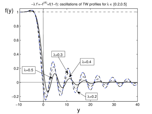
Figure 1. The TW profiles $f(y)$ of (1.19), (1.20) for $\lambda=0.2$, 0.3, 0.4, and 0.5.

In Figure 2, we show TW profiles for larger speeds $\lambda\in[0.6,1]$. All of them are clearly oscillatory as $y\to+\infty$. Concerning the type of convergence to 1 as $y\to-\infty$, it looks like it is monotone, but more close research below will show its oscillatory character to be justified by asymptotic expansion methods later on.

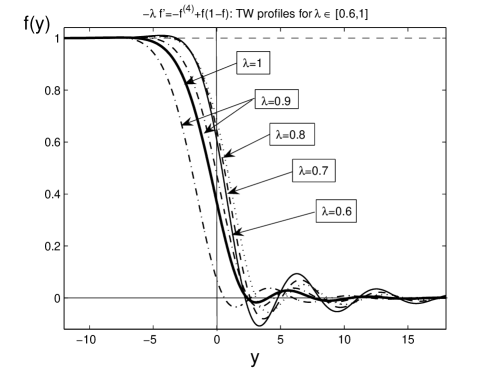
Figure 2. The TW profiles $f(y)$ of (1.19), (1.20) for $\lambda=0.6$, 0.7, 0.8, 0.9, and 1.

Both figures above confirm an important property:

(2.5) the oscillatory behaviour as $$y\to+\infty \lambda\uparrow$$ decreases as ;

see further comments below. Figure 3 shows the character of those oscillations for $\lambda=0.1$ on intervals $[0,300]$ (a) and $[0,600]$ (b).

Figure 4 confirms oscillatory convergence to 1 in the opposite limit, as $y\to-\infty$. While (a) still not that convincing and reveals just a single intersection with the equilibrium $f=1$, the (b), in the scale $10^{-5}$, shows further five intersections with 1. On better scales, we can detect a dozen of intersections at least, so the convergence to 1 is clearly oscillatory.

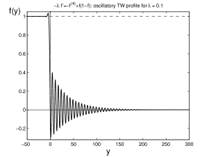
(a) oscillations on (0,300)

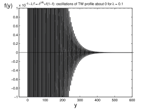
(b) oscillations on (0,600)

Figure 3. Oscillations of the TW profile $f(y)$ for $y\gg 1$; $\lambda=0.1$.

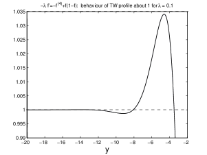
(a) scale $\sim 10^{-2}$

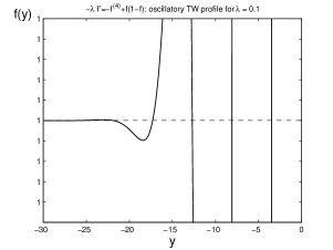
(b) scale $\sim 10^{-5}$

Figure 4. Illustration of an oscillatory convergence of the TW profile $f(y)$ to 1 for $y\ll-1$; $\lambda=0.1$.

Figure 5 shows TW profiles for $\lambda$ larger than 1. The phenomenon of a “maximal” speed (1.21) was clearly observed, with the following sharp estimate:

(2.6) $$1.27148\leq\lambda_{\rm max}(2)<1.27149.$$

In Figure 6, we show the profiles $f(y)$ for $\lambda$’s close to $\lambda_{\rm max}$ in (2.6). It turns out that, for $\lambda\approx\lambda_{\rm max}^{-}$, the TW profiles $f(y)$ remain oscillatory for $y\gg 1$, as Figure 6 confirms. Therefore, nonexistence of a $f(y)$ for $\lambda=\lambda_{\rm max}$ has nothing to do with a possible reduction of the dimension (from 3D to 2D) of the asymptotic bundle as $y\to+\infty$, when two complex roots of the characteristic equation become real; cf. Theorem 2.1(ii).

In Figure 7, we show the profile $f(y)$ for $\lambda=1.27148\approx\lambda_{\rm max}^{-}$, (a), and its oscillatory behaviour for $y\sim 35$, (b).

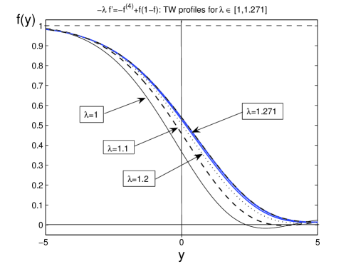
Figure 5. The TW profiles $f(y)$ of (1.19), (1.20) for $\lambda\in[1,1.271]$.

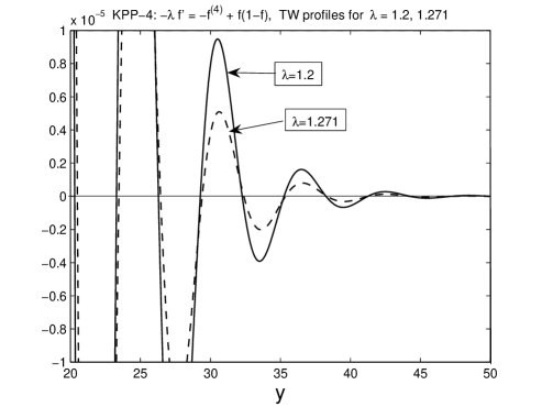
Figure 6. The TW profiles $f(y)$ of (1.19), (1.20) is becoming less oscillatory for $y\gg 1$ in the limit (2.6).

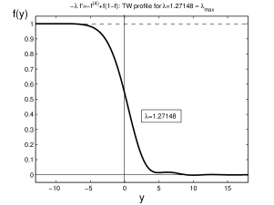
(a) $f(y)$

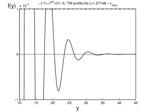
(b) oscillations for $y\sim 35$

Figure 7. Properties of the TW profile $f(y)$ for $\lambda=1.27148\approx\lambda_{\rm max}^{-}$.

In correlation with the second half of the statement in (1.21), we observed no TW profiles $f(y)$ for $\lambda>\lambda_{\rm max}$. It should be noted that, since we always take the Heaviside function (2.4) as the initial data for iterations via the bvp4c-solver, the non-convergence of the numerical scheme could reflect nonexistence of TWs satisfying the “minimal” requirement, with a “maximal” decay at infinity, which is available in the singular boundary conditions (1.20). In other words, for $\lambda>\lambda_{\rm max}$, there could be other TW profiles $f(y)$ with slower decay at infinity.

2.3. The exponential bundle as $y\to+\infty$: linearized analysis

In the present semilinear ($n=0$) case, such an analysis is reasonably easy, though, nowadays, a related stability theory using Evans functions have been developed for more complicated nonlinear systems; see [2], with a full list of references therein, with applications to general thin film flows.

Consider the linearized about zero ODE in (1.19):

(2.7) $$-\lambda g^{\prime}=-g^{(4)}+g.$$

The corresponding characteristic polynomials and equation take the form

(2.8) $$g(y)={\mathrm{e}}^{\mu y}\quad\Longrightarrow\quad H_{+}(\mu,\lambda)\equiv\mu^{4}-\lambda\mu-1=0.$$

The graph of the function $H_{+}(\mu,\lambda)$ for various $\lambda$ is shown in Figure 8. One can see that it keeps a similar form for all $\lambda>0$. It is seen that there exists a single real $\mu=\mu_{1}(\lambda)>0$ (the unstable mode), a single $\mu_{2}(\lambda)<0$ (a stable mode), and, for small $\lambda>0$, a complex stable mode with $\mu_{\pm}(\lambda)$ having ${\rm Re}\,\mu_{\pm}(\lambda)<0$.

Indeed, for $\lambda=0$ in (2.8), we get

(2.9) $$H_{+}(\mu,0)\equiv\mu^{4}-1=0\quad\Longrightarrow\quad\mu_{\pm}(0)=\pm{\mathrm{i}},$$

together with the stable $\mu_{1}(0)=-1$ and the unstable $\mu_{2}(0)=1$. The stable (unstable) roots for small $\lambda>0$ read

(2.10) $$\textstyle{\mu_{1}(\lambda)=-1-\frac{\lambda}{4+\lambda}+O(\lambda^{2})\quad\big{(}\mu_{2}(\lambda)=1+\frac{\lambda}{4-\lambda}+O(\lambda^{2})\big{)}.}$$

Similarly, the computations of complex roots of (2.8) yield

(2.11) $$\textstyle{\mu_{\pm}(\lambda)=-\frac{4\lambda}{\lambda^{2}+16}[1+O(\lambda)]\pm{\mathrm{i}}\big{[}1-\frac{\lambda^{2}}{\lambda^{2}+16}+O(\lambda^{3})\big{]}+O(\lambda^{3}),\,\,\,{\rm Re}\,\mu_{\pm}(\lambda)<0.}$$

Together with (2.10), this creates the whole 3D stable bundle of oscillatory linearized orbits, which we have seen in Figures 1 and 2.

Figure 9 shows that, according to (2.11), the TW profiles get more and more oscillatory when $\lambda$ approaches 0, i.e., when $\mu_{\pm}(\lambda)$ tend to pure imaginary roots in (2.9). The graph of $f(y)$ for $\lambda=0.01$ in Figure 9 was obtained by integration over the interval $[-50,6000]$; see also further results in the next subsection.

The above “local” results can be made global by using the following conclusion, that differs the KPP–4 problem from the KPP–2 one, for which multiple characteristic zeros take place at the minimal speed 2; see (1.7).

Proposition 2.2.

For any $\lambda\in\mathbb{R}$, the characteristic polynomial $\eqref{t6}$ does not admit a root of the algebraic multiplicity $2$.

Proof. Assume the contrary: there exist two coinciding roots $\bar{\mu}\in{\mathbb{C}}$, so that

$$\mu^{4}-\lambda\mu-1\equiv(\mu-\bar{\mu})^{2}(\mu^{2}+a\mu+b),\quad\mbox{with some constants $a,b\in{\mathbb{C}}$}.$$

Equating the coefficients of $\mu^{3}$, $\mu^{2}$, $\mu$, and 1 yields the system

(2.12) $$\left\{\begin{matrix}-2\bar{\mu}+a=0,\quad\,\,\,\,\,\,\\ \bar{\mu}^{2}-2a\bar{\mu}+b=0,\\ a\bar{\mu}^{2}-2b\bar{\mu}=-\lambda,\,\,\\ b\bar{\mu}^{2}=-1.\qquad\quad\,\end{matrix}\right.$$

Obtaining $a=2\bar{\mu}$ from the first equation and $b=-\frac{1}{\bar{\mu}^{2}}$ from the last one and substituting into the second one, we have

$$\textstyle{3\bar{\mu}^{2}+\frac{1}{\bar{\mu}^{2}}=0,}$$

so that $\bar{\mu}$ is a complex root. Then the third equation reads

$$\textstyle{\frac{3}{2}\,\lambda\bar{\mu}=-2,}$$

so that then $\lambda\in\mathbb{R}$ must be complex.  ∎

Thus, we claim the following result, which is sufficient for us for further applications:

Proposition 2.3.

(i) At least for all small $\lambda>0$, the linearized equation $\eqref{t5}$ $($and hence the KPP–$4$ one in $\eqref{E5}$ for $y\gg 1)$ admits a $3D$ stable family of oscillatory solutions as $y\to+\infty$, and a $1D$ unstable one of exponentially divergent orbits.

(ii) For small $\lambda<0$, the stable bundle as $y\to+\infty$ is $1D$, and the unstable one is $3D$.

Using Proposition 2.2, one can improve the case (i) to see that it might persist globally for $m=2$ for all $\lambda>0$. However, for some larger $m$, this might be not the case globally.

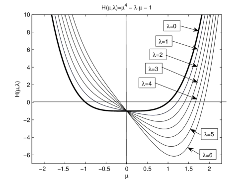
Figure 8. The graphs of the function $H_{+}$ in (2.8) for various $\lambda$.

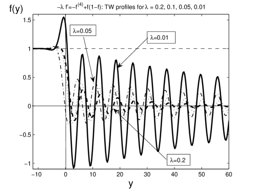
Figure 9. The TW profiles $f(y)$ of (1.19), (1.20) for $\lambda=0.2$, 0.1, 0.05, and 0.01.

2.4. Oscillatory singular limit $\lambda\to 0^{+}$

This has been discussed above. In fact, this is also a principle question concerning uniqueness of $\lambda$-branches of solutions. By careful numerical study of the behaviour of $f(y;\lambda)$ as $\lambda\to 0^{+}$ we rule out a possibility to have a saddle-node bifurcation at some small $\lambda_{\rm s-n}>0$, at which, via such a turning point, there appear two branches of TW profiles for $\lambda>\lambda_{\rm s-n}$.

In Figure 10, we show the TW profile $f(y)$ for $\lambda=0.005$, which gets very oscillatory for $y>0$. We thus claim that:

(2.13) there is no a saddle-node bifurcation for small $$\lambda>0$$ and

the $$\lambda \lambda\to 0^{+}$$-branch ends up as in a singular (oscillatory) limit.

Therefore, in general, nothing contradicts so far the existence of a single $\lambda$-branch of TW profiles. Of course, this well correlates with the nonexistence of a TW at $\lambda=0$ (Proposition 2.1) and some asymptotic computations above.

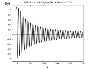
(a) on $(-20,250)$

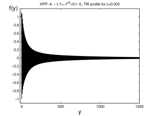
(b) on $(-20,1500)$

Figure 10. The highly oscillatory TW profile $f(y)$ for $\lambda=0.005$.

2.5. The 2D stable bundle as $y\to-\infty$

Then setting $f=1+g$ in (1.19) and linearizing yield the following characteristic equation:

(2.14) $$-\lambda g^{\prime}=g^{(4)}+g\quad\mbox{and}\quad g(y)={\mathrm{e}}^{\mu y}\quad\Longrightarrow\quad H_{-}(\mu,\lambda)\equiv\mu^{4}-\lambda\mu+1=0.$$

Therefore, for $\lambda=0$, we have 2D stable (${\rm Re}\,(\cdot)>0$) and unstable (${\rm Re}\,(\cdot)<0$) bundles with the roots

(2.15) $$\textstyle{\mu_{\pm}(0)=\pm\frac{1+{\mathrm{i}}}{\sqrt{2}}\quad\mbox{and}\quad\bar{\mu}_{\pm}(0)=\pm\frac{1-{\mathrm{i}}}{\sqrt{2}}.}$$

By continuity, for all small $\lambda>0$, there exists 2D stable manifold of the equilibrium 1 with the roots

(2.16) $$\textstyle{\mbox{stable bundle}:\quad\mu_{+}(\lambda)\quad\mbox{and}\quad\bar{\mu}_{+}(\lambda).}$$

Unlike Proposition 2.2, there exist multiple roots of the polynomial in (2.14), that follows from (2.12) with the last equation reading as $...=1$.

Proposition 2.4.

For the polynomial in $\eqref{t9}$, there exist two cases of double roots:

(2.17) $$\bar{\mu}_{\pm}=\pm 3^{-\frac{1}{4}}=\pm 1.3161...\quad\mbox{for}\quad\lambda_{\pm}=\pm 4\cdot 3^{-\frac{3}{4}}=\pm 9.1180...\,.$$

By (2.6), the positive value $\lambda_{+}$ in (2.17) (at which the bundles may exchange their dimensions) plays no role. Both bundles via (2.15) persists for small $\lambda>0$ ($\lambda<0$), so:

Proposition 2.5.

At least for all small $|\lambda|>0$, the linearized equation $\eqref{t9}$ $($and hence the KPP–$4$ one in $\eqref{E5}$ for $f\approx 1$ for $y\ll-1)$ admits a $2D$ stable family of oscillatory solutions as $y\to-\infty$, and a $2D$ unstable one of exponentially divergent orbits.

By Proposition 2.4, this result is global in $\lambda>0$, but this does not help to explain why at $\lambda_{\rm max}$ (“minimal”) TW profiles cease to exist.

2.6. Local blow-up to $-\infty$

In order to verify the global continuation properties of stable bundles, one needs to check whether the nonlinear ODE (1.19) admits blow-up and the dimension of such an unstable manifold. To this end, we re-write it down and, as usual, neglect the linear lower-order terms, which by standard local interior regularity are negligible for $|f|\gg 1$:

(2.18) $$f^{(4)}=-f^{2}+f+\lambda f^{\prime}=-f^{2}(1+o(1))\quad\mbox{as}\quad f\to\infty.$$

The unperturbed equation has the following exact solution:

(2.19) $$\textstyle{f^{(4)}=-f^{2}\quad\Longrightarrow\quad f_{0}(y)=-\frac{840}{(Y_{0}-y)^{4}}\to-\infty\quad\mbox{as}\quad y\to Y_{0}^{+},}$$

where $Y_{0}\in\mathbb{R}$ is a fixed arbitrary blow-up point. Studying the dimension of its stable manifold, we consider a perturbed solution and substitute it into the full equation (2.18) to get, on some linearization again:

(2.20) $$\textstyle{f=f_{0}+\varepsilon,\,\,|\varepsilon|\ll|f|\quad\Longrightarrow\quad(Y_{0}-y)^{4}\varepsilon^{(4)}-1680\varepsilon=-840+\frac{3360\lambda}{Y_{0}-y}+...\,.}$$

One can see that the leading solution consists of balancing the first two and the last term, that gives uniquely

(2.21) $$\textstyle{\varepsilon(y)=-\frac{140\lambda}{69}\,\frac{1}{Y_{0}-y}+...\,.}$$

Hence, in this expansion, no extra arbitrary parameter occurs. Thus, we arrive at:

Proposition 2.6.

For the ODE $\eqref{E5}$, the stable manifold of blow-up solutions is 1D depending on a single parameter being their blow-up point $Y_{0}\in\mathbb{R}$.

2.7. Some general conclusions

The KPP–4 ODE is difficult for an analytic study in the corresponding four-dimensional phase-space, so we do not plan here to perform its detailed and complete study.

However, the above local and blow-up analysis allows us to formulate some important consequences. Recall that equation (1.19) comprises analytic nonlinearities only, so by classic ODE theory [8], all dependencies on parameters in our problem are given by analytic functions.

Theorem 2.1.

Fix a $\lambda\in\mathbb{R}_{+}$ in the ODE problem $\eqref{E4}$, $\eqref{E5}$:

(i) If the dimension of the stable bundle as $y\to+\infty$ is $3D$ $($as in Proposition $\ref{Pr.osc1}(i))$, and $2D$ as $y\to-\infty$ $($as in Proposition $\ref{Pr.osc2})$, then the number of solutions $f(y)$ of the ODE problem $\eqref{E5}$, $\eqref{BC1}$ is not more than finite.

(ii) If the stable dimension of the bundle as $y\to+\infty$ changes to $2D$, or even becomes $1D$ $($as in Proposition $\ref{Pr.osc1}(ii)$ for $\lambda<0)$, then, most probably, the KPP–$4$ problem does not have a solution.

Proof. (i) Denote by $C_{\rm st}^{(1,2,3)}$ the real coefficients that control the 3D stable bundle at $y\to+\infty$, and by $D_{\rm unst}^{(1,2)}$ the coefficients of the 2D unstable bundle as $y\to-\infty$. Bearing in mind all three Propositions above, to get a global solution $f(y)$, one has to solve the following algebraic system:

(2.22) $$\left\{\begin{matrix}Y_{0}(C_{\rm st}^{(1,2,3)})=-\infty,\qquad\qquad\,\,\,\vskip 3.0pt plus 1.0pt minus 1.0pt\\ D_{\rm unst}^{(l)}(C_{\rm st}^{(1,2,3)})=0,\quad l=1,2,\end{matrix}\right.$$

where the first equation means that blow-up does not occur at finite points and hence “$Y_{0}=-\infty$” is to be understood in a limit sense (the solution remains uniformly bounded). Hence, we arrive at a system of three analytic equations with three unknowns $C_{\rm st}^{(1,2,3)}$. Then number of solutions is not more than countable, and the set of solutions is discrete with a possible accumulation point at infinity only.

Moreover, by our blow-up analysis above, it follows that, since the stable modes as $y\to+\infty$ are linearly independent, blow-up always occurs, if these coefficients $C_{\rm st}^{(1,2,3)}$ take sufficiently large values (a stability property of blow-up for quadratic ODE (2.18)). Therefore, all the solutions of (2.22) belong to a large “box” in $\mathbb{R}^{3}$, where only a finite number of those are available.

(ii) The result is obvious: then the corresponding analytic system becomes overdetermined (more equations than the unknowns), so it is inconsistent with the probability 1, meaning that its solvability(if any) can be “accidental” only and then is destroyed by a.a. arbitrary perturbations of any of the coefficients/functions involved (no structural stability). ∎

2.8. Existence: shooting from $y=-\infty$

Actually, the system (2.22) corresponds to “shooting from the right to the left-hand side” that was not principal for such an algebraic analysis. However, for a complete proof it is easier to shoot from $y=-\infty$. Indeed, keeping the same notations of “stable” expansion coefficients, we then arrive at two algebraic equations only:

(2.23) $$\left\{\begin{matrix}Y_{0}(D_{\rm st}^{(1,2)})=+\infty,\vskip 3.0pt plus 1.0pt minus 1.0pt\\ C_{\rm unst}(D_{\rm st}^{(1,2)})=0,\end{matrix}\right.$$

where we have used the fact that, at $y=+\infty$, there exists a 1D unstable manifold governed by the unique coefficient $C_{\rm unst}$. Thus, we obtain a system of two equations with two unknowns $D_{\rm st}^{(1,2)}$, and such a system admits a rather straightforward analysis on this plane. We refer, as a typical example, to [16, § 4], where a rather similar geometric-type analysis applied to a fourth-order ODE arising from a semilinear Cahn–Hilliard equation. See also [15, § 7] concerning ODEs in thin film theory.

The strategy is as follows. For a fixed $D_{\rm st}^{(1)}$, we use the second parameter $D_{\rm st}^{(2)}$ to satisfy the first equation in (2.23). It is clear that this is always possible, since in both limits $D_{\rm st}^{(2)}\to\pm\infty$, the solution $f(y;D_{\rm st}^{(1,2)})$ blows up, so that it is global for at least one value named $\hat{D}_{\rm st}^{(2)}(D_{\rm st}^{(1)})$. As the next step, we start to vary $D_{\rm st}^{(1)}$ to get rid of the unstable component as $y\to+\infty$, i.e., to satisfy the second equation in (2.23). In view of a clear oscillatory character of all the solutions as $y\to+\infty$, this always can be done.

Thus, the existence of a proper TW profile only is not a principal difficulty, but uniqueness remains a hard open problem still. We do not know any mathematical reason (in particular, a kind of a monotonicity property, usually leading to uniqueness), for which it must be unique. But numerically, we multiply observed convergence to the same profile from variously perturbed initial data as a starting point of nonlinear iterations.

3. The KPP–(6,1) problem

We now, more briefly than above, consider the KPP–(6 ,1) problem (1.22) and its ODE counterpart (1.23), (1.20). Of course, (2.1) remains valid, so we check existence of TWs for $\lambda>0$ only.

3.1. Numerical results

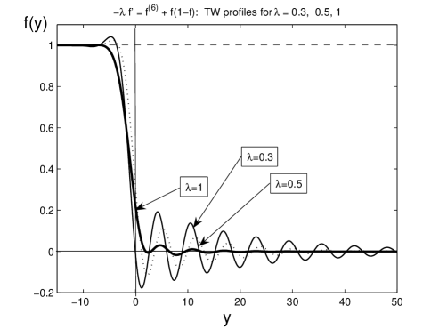
Figure 11. The TW profiles $f(y)$ satisfying (1.23), (1.20) for $\lambda=0.3$, 0.5, and 1.

Figure 11 shows TW profiles for $\lambda=0.3,\,\,0.5,$ and 1. In Figure 12, TW profiles are shown for larger speeds $\lambda\in[1,1.35]$. All of them are clearly oscillatory as $y\to+\infty$. Next, in Figure 13, we show TW profiles for larger $\lambda>1.4$.

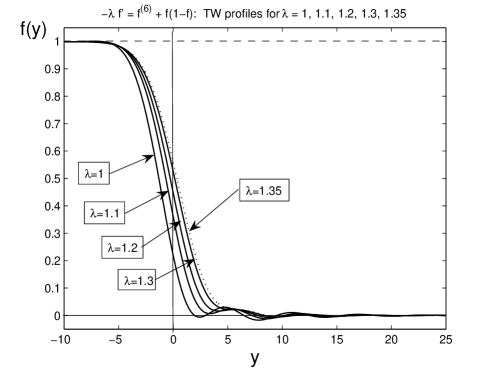
Figure 12. The TW profiles $f(y)$ of (1.23), (1.20) for $\lambda=1$, 1.1, 1.2, 1.3, and 1.35.

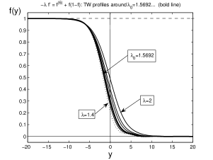
(a) TW profiles

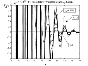
(b) oscillations for $y\gg 1$

Figure 13. TW profiles in the KPP–6 problem for $\lambda>1$.

Figure 13(a) confirms an oscillatory convergence to 1 in the opposite limit, as $y\to-\infty$. Figure (b) explains the same phenomenon as for the KPP–4 (cf. (2.6)), but here

(3.1) $$m=3:\quad 2.12110\leq\lambda_{\rm max}(3)<2.12111...\,,$$

at which TW profiles cease to exist. For $\lambda=2.12110$, the TW profile and its oscillations for $y\gg 1$ are shown in Figure 15.

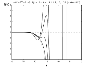
(a) convergence to 1

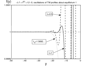
(b) oscillations for $\lambda_{*}=1.121...$

Figure 14. Oscillations of the TW profile $f(y)$ as $y\to\pm\infty$.

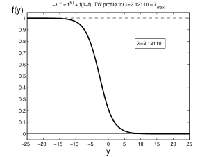
(a) $f(y)$

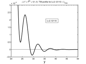
(b) oscillations for $y\sim 30$

Figure 15. Properties of $f(y)$ for $\lambda=2.12110$.

3.2. Dimensional analysis of the bundles and towards existence

This is not essentially more difficult than in the KPP–4 problem. Namely, consider the linearized about zero ODE in (1.23):

(3.2) $$-\lambda g^{\prime}=g^{(6)}+g.$$

The corresponding characteristic polynomial is now

(3.3) $$g(y)={\mathrm{e}}^{\mu y}\quad\Longrightarrow\quad H_{+}(\mu,\lambda)\equiv\mu^{6}+\lambda\mu-1=0.$$

The graph of the function $H_{+}(\mu,\lambda)$ for various $\lambda$ is shown in Figure 16. It is quite similar to that for the KPP–$(4,1)$. Moreover, Proposition 2.2 holds for the polynomial in (3.2).

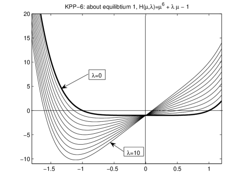
Figure 16. The graphs of the function $H_{+}$ in (3.3) for various $\lambda=0,1,2,...,10$.

Similarly, we study the bundles as $y\to-\infty$, where there occurs

(3.4) $$H_{+}(\mu,\lambda)\equiv\mu^{6}+\lambda\mu+1=0.$$

It admits double roots

(3.5) $$\bar{\mu}_{\pm}=\pm 5^{-\frac{1}{6}}=\pm 0.7647...\quad\mbox{at}\quad\lambda_{\pm}=\mp 2\cdot 5^{-\frac{5}{6}}=\mp 0.5231...\,,$$

which, again, have nothing to do with the maximal speed in (3.1).

Then, for small $|\lambda|>0$, the dimensions of stable/unstable manifolds correspond to a proper shooting, but with more parameters. Therefore, while we can prove that the family of TW profiles is not more than countable (or even finite), the actual proving of existence is more difficult for such a multi-dimensional shooting.

Note also, that the blow-up problem (cf. the ODE (2.19))

(3.6) $$f^{(6)}=f^{2}$$

is now more difficult since (3.6) admits oscillatory solutions, which can be studied as in [15, § 7] by introducing an oscillatory component represented by a periodic function.

4. Higher-order problems: KPP–(8,1) and KPP–(10,1)

Those are two examples to illustrate a possibility of such KPP extensions. By (2.1), one needs to consider $\lambda>0$ only.

Thus, in the KPP–(8,1), we have the following ODE problem:

(4.1) $$(\mbox{PDE})\quad u_{t}=-D_{x}^{8}u+u(1-u)\quad\Longrightarrow\quad(\mbox{ODE})\quad-\lambda f^{\prime}=-f^{(8)}+f(1-f).$$

Figure 17 shows TW profiles for $\lambda=0.5$, 1, and 2, satisfying the ODE (4.1) with the singular boundary conditions (1.20). The critical existence speed value in the sense of (1.21) is now

(4.2) $$m=4:\quad 2.107\leq\lambda_{\rm max}(4)<2.108.$$

Figure 18 shows $f(y)$ for $\lambda=2.107$ from (4.2), while Figure 19 explains its oscillations for $y\sim 35$.

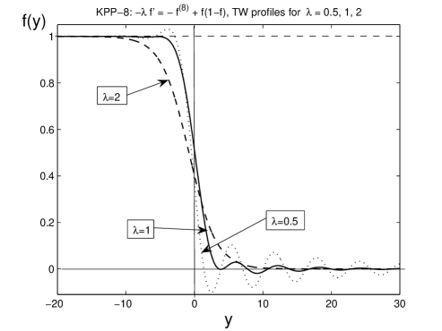
Figure 17. The TW profiles $f(y)$ satisfying (4.1), (1.20) for $\lambda=0.5$, 1, and 2.

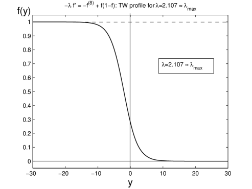
Figure 18. The TW profile $f(y)$ satisfying (4.1), (1.20) for $\lambda=2.107$.

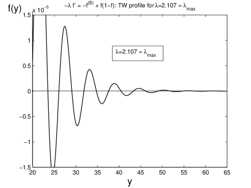
Figure 19. Oscillations of the TW profile $f(y)$ from Figure 18 for $\lambda=2.107$.

In the KPP–(10,1), we deal with the following ODE problem:

(4.3) $$(\mbox{PDE})\quad u_{t}=D_{x}^{10}u+u(1-u)\quad\Longrightarrow\quad(\mbox{ODE})\quad-\lambda f^{\prime}=f^{(10)}+f(1-f).$$

Figure 20 shows TW profiles for $\lambda=0.5$, 1 and 2, satisfying the ODE (4.3) with the boundary conditions (1.20).

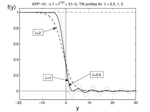
Figure 20. The TW profiles $f(y)$ satisfying (4.3), (1.20) for $\lambda=0.5$, 1, and 2.

It is seen that the TW profiles for both problems are close to each other. For instance, for $\lambda=0.5$, the difference is not more than $2\%$. This confirms that it is possible to pass to the limit $m\to+\infty$ in the $2m$th-order KPP–problem (1.24), (1.25), and construct an analogy of the KPP–problems for an “infinite-order” PDE and ODE.

A local stability of bundles can be done for both above parabolic models establishing for which $\lambda$’s the shooting problem is well posed and the corresponding algebraic systems are consistent. Indeed, proving existence, to say nothing of the uniqueness, are open problems.

5. The origin of $\log t$-shift: centre subspace balancing

In this section, we explain the origin of the $\log t$-shifting (retarding) from the TW for the PDE higher-order KPP–problem.

More correctly, the actual proof of such $\log t$-drift assumes a delicate matching of the solution behaviour on compact subsets in the TW $y$-variable, i.e., in the Inner Region, with a remote Outer Region for $y\gg 1$, where the influence of the nonlinear term $-u^{2}$ is negligible, and the actual behaviour is governed by the linear bi-harmonic operator. However, we do not present here this kind of a procedure of matching of asymptotic expansions of those two regions, which is difficult in the present quite general case.

Thus, we consider a KPP-type problem for a semilinear PDE

(5.1) $$u_{t}={\bf A}u+u(1-u)\quad\mbox{in}\quad\mathbb{R}\times\mathbb{R}_{+},$$

where ${\bf A}$ is a proper homogeneous isotropic linear differential operator satisfying some extra conditions specified below. For instance, we may fix, as a simple example, the bi-Laplacian operator

(5.2) $${\bf A}=-D_{x}^{4}\quad(\mbox{or $=D_{x}^{6}$, or $(-1)^{m+1}D_{x}^{2m}$, that is the same}).$$

5.1. Behaviour for small $t>0$: first appearance of $\log t$

Given the Heaviside data (1.2), to study (5.1), (5.2) (with $m=2$, but any $m\geq 2$ fits quite similarly) for small $t>0$, one needs to use the rescaled independent variables

(5.3) $$\textstyle{z=\frac{x}{t^{1/4}}\quad\mbox{and}\quad\tau=\log t\to-\infty\quad\mbox{as}\quad t\to 0^{+}.}$$

Then the rescaled equation takes the form

(5.4) $$\textstyle{v_{\tau}=\big{(}{\bf B}-\frac{1}{4}\,I\big{)}+{\mathrm{e}}^{\tau}\,v(1-v),\quad\mbox{where}\quad{\bf B}=-D_{z}^{4}+\frac{1}{4}\,zD_{z}+\frac{1}{4}\,I.}$$

Denoting by $V(z)$ the unique stationary solution of the problem

(5.5) $$\textstyle{\big{(}{\bf B}-\frac{1}{4}\,I\big{)}V=0\quad\mbox{in}\quad\mathbb{R},\quad V(-\infty)=1,\quad V(+\infty)=0,}$$

and performing the standard linearization in (5.4) yield

(5.6) $$\textstyle{v=V+w\quad\Longrightarrow\quad w_{\tau}=\big{(}{\bf B}-\frac{1}{4}\,I\big{)}+{\mathrm{e}}^{\tau}\,V(1-V)+...\,,}$$

provided that $|w|\ll 1$. Finally, in such an inner region, we obtain

(5.7) $$\textstyle{w(z,\tau)={\mathrm{e}}^{\tau}\varphi(z)+...\quad\Longrightarrow\quad\big{(}{\bf B}-\frac{1}{4}\,I\big{)}\varphi=h(z)\equiv-V(z)(1-V(z)).}$$

According to the linearized analysis in Section 2, $h(z)$ has an exponential decay at infinity, so, keeping the leading terms, we may assume that

(5.8) $$h(z)=B_{-}{\mathrm{e}}^{b_{-}z}+...\quad\mbox{as}\quad z\to-\infty\quad\mbox{and}\quad h(z)=B_{+}{\mathrm{e}}^{b_{+}z}+...\quad\mbox{as}\quad z\to+\infty,$$

where $B_{\pm},\,b_{\pm}\not=0$ are some constants and ${\rm Re}\,b_{-}>0$ and ${\rm Re}\,b_{+}<0$.

Since ${\bf B}$ is known to possess a discrete spectrum in a weighted $L^{2}_{\rho}$-space [13], where

(5.9) $$\rho(z)={\mathrm{e}}^{a_{0}|z|^{4/3}},\quad a_{0}>0\,\,\,\mbox{is a small constant},$$

and a complete set of eigenfunctions $\{\psi_{k}\}$, the problem for $\varphi$ in (5.7) admits the unique solution given by the eigenfunction expansion

(5.10) $$\textstyle{\varphi=\sum c_{k}\psi_{k},\quad\mbox{where}\quad c_{k}=\langle h,\psi_{k}^{*}\rangle,}$$

$\{\psi_{k}^{*}\}$ being the eigenfunction set of generalized Hermite polynomials as eigenfunctions of the adjoint operator

(5.11) $$\textstyle{{\bf B}^{*}=-D_{z}^{4}-\frac{1}{4}\,zD_{z}.}$$

In (5.10), $\langle\cdot,\cdot\rangle$ is the dual $L^{2}$-metric, in which (5.11) represents the adjoint to ${\bf B}$. By (5.8), all such integrals converge. Moreover, one can check that

(5.12) $$\textstyle{\varphi(z)=\frac{4B_{\pm}}{b_{\pm}z}\,{\mathrm{e}}^{b_{\pm}z}+...\quad\mbox{as}\quad z\to\pm\infty.}$$

Thus, we obtain the following expansion of the solution $u(x,t)$ for the Heaviside initial function:

(5.13) $$\textstyle{u(x,t)=V\big{(}\frac{x}{t^{1}/4}\big{)}+t\,\varphi\big{(}\frac{x}{t^{1}/4}\big{)}+...\,,\quad\mbox{in the domain, where}\,\,\,\big{|}t\,\varphi\big{(}\frac{x}{t^{1}/4}\big{)}\big{|}\ll 1.}$$

Hence, the last linearization condition defines the domain of its applicability: by (5.13),

(5.14) $$\textstyle{|t\,\varphi(z)|\ll 1\quad\Longrightarrow\quad|t{\mathrm{e}}^{b_{\pm}x/t^{1}/4}|\ll 1\quad\Longrightarrow\quad|x|\ll t^{\frac{1}{4}}\,|\log t|.}$$

Here, we first observe the appearance of the $\log t$-“shift” (now, a factor) in the rescaled variable coming from the inner expansion region. However, a further extension of such an expansion towards a proper TW-frame (to see how this $\log t$-multiplier is actually transformed into the $logt$-shift) is a difficult procedure, which we cannot treat here. Instead, below, we will catch this $\log t$-shift in a simpler way, starting now directly from the TW-frame.

5.2. TW-frame: linearization and rescaled equation

We now perform a perturbation analysis in the TW-frame. Then, we need to assume that the corresponding ODE problem

(5.15) $$-\lambda_{0}f^{\prime}={\bf A}f+f(1-f),$$

with the conditions (1.20), admits a unique solution $f$. Then, attaching the solution $u(x,t)$ to the front moving and setting, for convenience, $x_{f}(t)\equiv\lambda_{0}t-g(t)$, the PDE reads

(5.16) $$u(x,t)=v(y,t),\quad y=x-\lambda_{0}t+g(t)\quad\Longrightarrow\quad v_{t}={\bf A}v+\lambda_{0}v_{y}+v(1-v)-g^{\prime}(t)v_{y}.$$

We next linearize (5.16) by setting

(5.17) $$v(y,t)=f(y)+w(y,t),$$

that yields the following perturbed equation:

(5.18) $$w_{t}={\bf B}w-g^{\prime}(t)f^{\prime}-g^{\prime}(t)w_{y}-w^{2},\,\,\,\mbox{where}\,\,\,{\bf B}w={\bf A}w+(1-2f)w+\lambda_{0}w_{y}.$$

Assuming that, in this $g(t)$-moving frame, there exists the convergence as in (1.12), so that $w(t)\to 0$ as $t\to+\infty$, one can see that the leading non-autonomous perturbation in (5.18) is the second term on the right-hand side. However, as we show, the last two terms, though negligible, will define a proper $\log t$-shift of the front.

5.3. Where $\log t$-shift comes from

First of all, an extra “centre manifold”-like front shifting can be connected with the known results on the instability of travelling waves in a number of analogous fourth and sixth-order parabolic equations; see [35, 52, 46] and references there in. However, of course, this does not directly imply specifically the $logt$-shifting to be justified. In addition, it was always shown that, typically, the corresponding linearized operators (like ${\bf B}$) possess continuous spectra, the fact that essentially complicates our further analysis.

In this connection, note also that the rescaled equation (5.18) is essentially non-autonomous in time, so we can hardly use powerful tools of nonlinear semigroup theory; see [47]. However, using a formal asymptotic approach, we will trace out some typical features of a centre subspace behaviour, after an extra rescaling and balancing of non-autonomous perturbations.

Thus, as usual (see Introduction), we assume that $g^{\prime}(t)\to 0$ as $t\to+\infty$ sufficiently fast, i.e., at least algebraically, so that

(5.19) $$|g^{\prime\prime}(t)|\ll|g^{\prime}(t)|\quad\mbox{for}\quad t\gg 1.$$

Under the hypothesis (5.19), the only possible way to balance all the terms therein (including the quadratic one $-w^{2}$) for $t\gg 1$ is to assume the asymptotic separation of variables:

(5.20) $$w(y,t)=g^{\prime}(t)\psi(y)+\varepsilon(t)\varphi(y)+...,\quad\mbox{where}\quad|\varepsilon(t)|\ll|g^{\prime}(t)|\quad\mbox{as}\quad t\to+\infty.$$

Here, we omit higher-order perturbations. Substituting (5.20) into (5.20) yields

(5.21) $$g^{\prime\prime}(t)\psi+\varepsilon^{\prime}(t)\varphi+...=\,g^{\prime}(t)({\bf B}\psi-f^{\prime})\vskip 3.0pt plus 1.0pt minus 1.0pt$$

$$+\varepsilon(t){\bf B}\varphi-(g^{\prime}(t))^{2}(\psi^{\prime}+\psi^{2})-g^{\prime}(t)\varepsilon(t)(\varphi^{\prime}+2\varphi\psi)-\varepsilon^{2}(t)\varphi^{2}+...\,.$$

Using (5.19) and (5.20) in balancing first the leading terms of the order $O(g^{\prime}(t))$ yields the elliptic equation for $\psi$:

(5.22) $$\textstyle{O(g^{\prime}(t))\,\,\big{(}=O(\frac{1}{t})\big{)}:\quad{\bf B}\psi-f^{\prime}=0.}$$

Then balancing the rest of the terms in (5.21) requires their asymptotic equivalence,

(5.23) $$\textstyle{g^{\prime\prime}(t)\sim-(g^{\prime}(t))^{2}\sim\varepsilon(t),\,\,\,\mbox{i.e.,}\,\,\,g(t)=k\log t,\,\,\mbox{$g^{\prime}(t)=\frac{k}{t},\,\,g^{\prime\prime}(t)=-\frac{k}{t^{2}}$,}\,\,\varepsilon(t)=\frac{1}{t^{2}}.}$$

Then, we obtain the second inhomogeneous singular Sturm–Liouville problem for $\varphi$:

(5.24) $$\textstyle{O\big{(}\frac{1}{t^{2}}\big{)}:\quad{\bf B}\varphi=k\psi+k^{2}(\psi^{\prime}+\psi^{2}).}$$

Thus, the first simple asymptotic ODE in (5.23) gives the $\log t$-dependence as in (1.15). Finally, we arrive at the following system for $\{\psi,\varphi\}$:

(5.25) $$\left\{\begin{aligned} &{\bf B}\psi=f^{\prime},\\ &{\bf B}\varphi=k\psi+k^{2}(\psi^{\prime}+\psi^{2}).\end{aligned}\right.$$

Solving this system, with typical boundary conditions as in (1.20), allows then to continue the expansion of the solutions of (5.18) close to an “affine (i.e., shifted via $f^{\prime}$ on the RHS) centre subspace” of ${\bf B}$ governed by the spectral pair obtained by translation in (5.15):

(5.26) $$\hat{\lambda}_{0}=0\quad\mbox{and}\quad\hat{\psi}_{0}(y)=f^{\prime}(y).$$

The asymptotic expansion for $t\gg 1$ then takes the form

(5.27) $$\textstyle{w(y,t)=\frac{k}{t}\,\psi(y)+\frac{1}{t^{2}}\,\varphi(y)+...\,,}$$

which can be easily extended by introducing further terms, with similar inhomogeneous Sturm–Liouville problems for the expansion coefficients.

Final “spectral” remark: on $k$-values. Thus, ${\bf B}$ does not have a discrete spectrum (see references at the beginning of Section 5.3), so one cannot get a simple algebraic equation for $k$ by demanding the standard orthogonality of the right-hand side in the second equation in (5.25) to the adjoint eigenvector $\hat{\psi}^{*}_{0}$ of ${\bf B}^{*}$ in the $L^{2}$-metric (in which the adjoint operator ${\bf B}^{*}$ is obtained), like

(5.28) $$k:\quad\langle k\psi+k^{2}(\psi^{\prime}+\psi^{2}),\,\hat{\psi}_{0}^{*}\rangle=0.$$

Therefore, the system (5.25) cannot itself determine the actual value of $k$ therein. As we have mentioned, the latter requires a difficult matching analysis of Inner and Outer Regions, which, for the KPP–4 (and all other problems), remains an open problem.

5.4. On some other related results and references

It is worth mentioning that, in similar cases, it is known that, after a suitable time-rescaling and necessary transformations, the orbit can approach the center subspace ${\rm Span}\{\hat{\psi}_{0}\}$ locally in space (in $L^{2}_{\rho,{\rm loc}}$). First results for the semilinear heat equation

$$u_{t}=\Delta u-u^{p}\quad\quad\mbox{in}\quad\mathbb{R}^{N}\times\mathbb{R}_{+}\quad(u>0)$$

treated in such a way were proved in [36, 43, 26, 5], etc. in the middle of the 1980s; a full list of references is given in [51, Ch. 2]; see also various chapters in [33]. The first realization of the scaling idea in quasilinear degenerate parabolic equations, which is one of the powerful tools to study such a stabilization was established by Kamin in 1973, [42]. Sometimes, it is called now a renormalization group method. Basic ideas go back to the dimensional ideas in nonlinear problems and to the notion of self-similarity of the second kind introduced by Ya.B. Zel’dovich at the beginning of the 1950s. See Barenblatt’s book [1], where several such ideas were discussed first. Of course, it should be noted that rigorous results obtained in the above papers are always related to semilinear and quasilinear second-order parabolic equations and are heavily based on the Maximum Principle. Therefore, any justification of such approaches to bi- and poly-harmonic equations is expected to be very difficult.

One can see that the above elementary conclusion well corresponds to an “(affine) centre subspace analysis” of the non-autonomous PDE (5.18), and then $\tau=\log t$ naturally becomes the corresponding “slow” time variable; see various examples in [31, 32, 33] of such a slow motion along centre subspaces in nonlinear parabolic problems with global and blow-up solutions. In the latter case, the slow time variable is

$$\tau=-\ln(T-t)\to+\infty\quad\mbox{as $t$ approaches finite blow-up time $T^{-}$}.$$

For the semilinear higher-order reaction-absorption equations such as

(5.29) $$u_{t}=-u_{xxxx}-|u|^{p-1}u\quad\mbox{in}\quad\mathbb{R}\times\mathbb{R}_{+},\quad\mbox{with}\quad p>1,$$

existence of $\log t$-perturbed global asymptotics was established in [21]. For finite-time extinction, with $-1<p<1$ in (5.29), this was done in [23]. For the corresponding blow-up problem with the combustion source

$$u_{t}=-u_{xxxx}+|u|^{p-1}u\quad\mbox{in}\quad\mathbb{R}\times\mathbb{R}_{+},\quad\mbox{with}\quad p>1,$$

centre manifold-like $\log(T-t)$-dependent blow-up singularities were constructed in [20]. We must admit that a justification of such $\log t$-corrections in any of KPP–$2m$ problems with $m\geq 2$ is more difficult and has been obtained for global orbits as $t\to+\infty$. For blow-up orbits, with $|\log(T-t)|$, this remains an open problem.

6. When the $\omega$-limit set consists of TW profiles

Consider the $2m$th-order KPP problem for the PDE (1.24), with smooth bounded “step-like” initial data,

(6.1) $$u(x,0)=u_{0}(x)\quad\mbox{in}\quad\mathbb{R}:\quad u_{0}(x)\to 0,\,\,\,x\to+\infty\quad\mbox{and}\quad u_{0}(x)\to 1,\,\,\,x\to-\infty,$$

where the convergence is assumed to be sufficiently exponentially fast.

Theorem 6.1.

Let (1.24), (6.1) admit a global uniformly bounded solution $u(x,t)$ having a “step-like” form for all $t\gg 1$, i.e.,

(6.2) $$u(x,t)\to 0\quad\mbox{as}\quad x\to+\infty,\quad u(x,t)\to 1\quad\mbox{as}\quad x\to-\infty$$

sufficiently exponentially fast uniformly in $t\gg 1$. Let, for all $t\gg 1$, the front location $x_{f}(t)$ can be uniquely and smoothly $($say, analytically$)$ defined from the equation

(6.3) $$\textstyle{u(x_{f}(t),t)=\frac{1}{2}\quad\mbox{for}\quad t\gg 1,}$$

with the following asymptotic representation:

(6.4) $$x_{f}(t)=\lambda_{0}t-g(t),\quad\mbox{where}\quad g^{\prime}(t)\to 0\quad\mbox{as}\quad t\to+\infty,$$

where $\lambda_{0}>0$ is a constant. Then $\lambda_{0}\in\Lambda$, i.e., there is a TW profile (maybe, non-unique) $f(\cdot;\lambda_{0})$ satisfying the ODE $\eqref{m2}$, with $\eqref{BC1}$, and the omega-limit set $\omega(u_{0})$, defined via uniform convergence in the TW frame $y=x-\lambda_{0}t+g(t)$, is contained in this connected closed family of TW profiles:

(6.5) $$\omega(u_{0})\subseteq\{f(\cdot;\lambda_{0})\}.$$

Proof. (i). Given a sequence $\{t_{k}\}\to+\infty$, passing to the limit(in a weak sense, implying, by parabolic regularity, stronger convergence) in the rescaled perturbed equation (5.16) as $\{t_{k}+s\}\to+\infty$, one concludes that

(6.6) $$v(\cdot,t_{k}+s)\to w(\cdot,s)\quad\mbox{in, say,}\quad L^{\infty}_{\rm loc}(\mathbb{R};\mathbb{R}_{+})\quad(\mbox{or in $C_{\rm loc}(...)$, etc.}),$$

where, by the assumption in (6.4), $w(y,s)$ solves (in the classic sense) the corresponding unperturbed equation

(6.7) $$w_{s}={\bf A}w+\lambda_{0}w_{y}+w(1-w)\quad\mbox{in}\quad\mathbb{R}\times\mathbb{R}_{+},$$

with data $w_{0}\in\omega(u_{0})$. Moreover, by the definition of the front tracking (6.3),

(6.8) $$\textstyle{w(0,s)\equiv\frac{1}{2}\quad\Longrightarrow\quad D_{s}^{k}w(0,s)=0\quad\mbox{for any}\quad k=1,2,3,...\,.}$$

Since the solutions of (6.6) are analytic in both $y$ and $s$ for $s>0$ [18] (see also related more recent results in [47]), (6.8) implies that $w(y,s)$ is independent of $s$, so, under the above hypothesis, $w(y,s)\equiv f(y;\lambda_{0})$.  ∎

Remark: Blow-up in the parabolic problem is possible. The conditions on data $u_{0}(x)$ at the beginning of Theorem 6.1 are essential. Indeed, if $-u_{0}^{2}(x)\ll u_{0}(x)\leq-1$ on some interval, then any such solution blows-up in finite time as $t\to T^{-}\in\mathbb{R}_{+}$:

(6.9) $$\textstyle{\lim_{t\to T^{-}}\,\,\sup_{x\in\mathbb{R}}|u(x,t)|=+\infty.}$$

Different proofs can be found in [12, 29]. Then blow-up can be self-similar [3] and then blow-up is not uniform, i.e.,

(6.10) $$\textstyle{\lim_{t\to T^{-}}\,\,\inf_{x\in\mathbb{R}}u(x,t)=-\infty\quad\mbox{and}\quad}\textstyle{\lim_{t\to T^{-}}\,\,\sup_{x\in\mathbb{R}}u(x,t)=+\infty.}$$

As an alternative, blow-up may create centre and stable manifold patterns, [20].

Remark 1: Is the $\omega$-limit set a point? – No answer. For various smooth (or analytic) gradient systems, under some extra assumptions, it is known that the omega limit sets consists of a single point. We refer to, e.g., as a first such result, to Hale–Raugel’s approach that applies to guarantee convergence of the orbits of gradient systems; see [37], where a survey and further references are given. This approach essentially relies on spectral properties of the linearized operator (main Hale–Raugel’s hypothesis is that the equilibrium has multiplicity at most one, or $k>1$ under special hypothesis) and uses properties of stable, unstable, and center manifolds, that are difficult to justify for some less smooth equations. We also refer to [6], where a similar approach to stabilization is used and other references can be found.

An alternative application is the Łojasiewicz–Simon approach to parabolic equations. Namely, the Łojasiewicz–Simon inequality is an effective tool of studying of the stabilization phenomena in various evolution problems. In particular, it completely settles the case of analytic nonlinearities; see references in [7]; see also [17, 39, 40, 54, 56] and references therein. Another approach [30] is based on Zelenyak’s ideas (1968) [57] from one dimension that are mainly connected with Lyapunov functions only for gradient dynamical systems; see also a short survey and references in [30].

Unfortunately, (6.7) is not a gradient system in the usual and necessary sense (and (5.16) is a not a “perturbed” one, for which there exists a Lyapunov-like functional that is “almost” monotone on evolution orbits). In fact, the bi-harmonic equation (1.18) (as well as any of (1.24)) admits a “pseudo-Lyapunov function”, obtained, as usual, by multiplication of the equation by $u_{t}$ in $L^{2}$:

(6.11) $$\textstyle{\frac{\mathrm{d}}{{\mathrm{d}}t}\,L[u](t)\equiv\frac{\mathrm{d}}{{\mathrm{d}}t}\,\big{[}\frac{1}{2}\int(u_{xx})^{2}+\int\big{(}c(x)-\frac{1}{2}\,u^{2}+\frac{1}{3}\,u^{3}\big{)}=\int(u_{t})^{2}\leq 0,}$$

where $c(x)$ is any smooth function with an exponential convergence as $x\to\infty$ satisfying, for the sake of convergence of the second integral in (6.11),

(6.12) $$\textstyle{c(-\infty)=\frac{1}{6}\quad\mbox{and}\quad c(+\infty)=0.}$$

Unfortunately, $L[u](t)$ is not bounded below, so cannot be used in the Lyapunov classical analysis. This is also easily seen in the TW frame, where, for $v=v(y,s)$, (6.11) reads

(6.13) $$\textstyle{\frac{\mathrm{d}}{{\mathrm{d}}t}\,\big{[}\frac{1}{2}\int(v_{xx})^{2}+\int\big{(}c(y+\lambda_{0}t-g(t))-\frac{1}{2}\,u^{2}+\frac{1}{3}\,u^{3}\big{)}=\int(v_{t}-\lambda_{0}v_{y}-g^{\prime}(t)v_{y})^{2}\leq 0.}$$

Observe that, here, $c(y+\lambda_{0}t-g(t))\to 0$ as $t\to+\infty$ uniformly on compact subsets in $y$. Since such a Lyapunov function has almost nothing to do with TW profiles (i.e., equilibria), we do not think that these inequalities can be of any help in the stabilization problem.

On the other hand, for generalized gradient KPP-problems in Appendix A, where the ODEs for $f$ are variational, these approaches can apply; see comments therein.

Acknowledgement. The author would like to thank D. Williams, as well as other active participants of seminars of Reaction-Diffusion and Probability Groups, Department of Mathematical Sciences, University of Bath, who stimulated a number of discussions of PDE aspects of the KPP–2 problem in 1995, which led the author to initiate such a research, [19].

Appendix A. Some modified variational KPP-problems

A.1. A more general semilinear bi-harmonic equation

Consider the following bi-harmonic equation, with parameters $\alpha,\beta,\gamma\in\mathbb{R}$:

(A.1) $$\mbox{(PDE)}: u_{t}=-u_{xxxx}+\alpha u_{xxx}+\beta u_{xx}+\gamma u_{x}+u(1-u),$$

$$\mbox{(ODE)}: \hat{\bf A}f\equiv-f^{(4)}+\alpha f^{\prime\prime\prime}+\beta f^{\prime\prime}+(\lambda+\gamma)f^{\prime}=-f(1-f).$$

Proposition A.1.

For a fixed $\lambda\in\mathbb{R}$, the ODE in (A.1) is $($formally$)$ variational in the metric of the weighted space $L^{2}_{\rho}(\mathbb{R})$, where

(A.2) $$\textstyle{\rho={\mathrm{e}}^{-\frac{\alpha y}{2}}\quad\mbox{and $\alpha\in\mathbb{R}$ solves the cubic equation}\quad\frac{\alpha}{2}\big{(}\frac{\alpha^{2}}{4}+\beta\big{)}=-(\lambda+\gamma).}$$

Proof. Using the general form of symmetric (self-adjoint) ordinary differential operators [48], we have to find two coefficients $p_{1}(y)$, $p_{2}(y)$, and the weight $\rho(y)$ such that

(A.3) $$\textstyle{\hat{\bf A}f\equiv-\frac{1}{\rho}\,[(p_{1}f^{\prime\prime})^{\prime\prime}+(p_{2}f^{\prime})^{\prime}]\equiv-\frac{1}{\rho}\,[p_{1}f^{(4)}+2p_{1}^{\prime}f^{\prime\prime\prime}+(p_{1}^{\prime\prime}+p_{2})f^{\prime\prime}+p_{2}^{\prime}f^{\prime}].}$$

This yields the following system of linear differential equations:

(A.4) $$\left\{\begin{aligned} &\textstyle{\frac{p_{1}}{\rho}=1},\\ &\textstyle{\frac{2p_{1}^{\prime}}{\rho}=-\alpha},\\ &\textstyle{\frac{p_{1}^{\prime\prime}+p_{2}}{\rho}=-\beta},\\ &\textstyle{\frac{p_{2}^{\prime}}{\rho}=-(\lambda+\gamma)}.\end{aligned}\right.$$

Hence, $p_{1}=\rho$, so, the second equation yields the positive weight in (A.2):

(A.5) $$\textstyle{\frac{2\rho^{\prime}}{\rho}=-\alpha\quad\Longrightarrow\quad\rho(y)={\mathrm{e}}^{-\frac{\alpha y}{2}}>0.}$$

The third equation then defines

(A.6) $$\textstyle{p_{2}=-p_{1}^{\prime\prime}-\beta\rho=-\rho^{\prime\prime}-\beta\rho=-\big{(}\frac{\alpha^{2}}{4}+\beta\big{)}\,{\mathrm{e}}^{-\frac{\alpha y}{2}}.}$$

Finally, the last equation in (A.4) yields the necessary condition on $\alpha$:

(A.7) $$\textstyle{p_{2}^{\prime}=-(\lambda+\gamma)\rho\quad\Longrightarrow\quad p_{2}(y)=\frac{2}{\alpha}\,(\lambda+\gamma)\,{\mathrm{e}}^{-\frac{\alpha y}{2}},}$$

i.e., comparing with $p_{2}$ in (A.6) gives the cubic algebraic equation in (A.2).  ∎

Thus, expressing all the coefficients in (A.3) in terms of the weight $\rho$ given in (A.2) yields the following problem with a symmetric operator:

(A.8) $$\textstyle{\hat{\bf A}f\equiv-\frac{1}{\rho}\,\big{[}(\rho f^{\prime\prime})^{\prime\prime}+\frac{\lambda+\gamma}{\alpha}\,(\rho f^{\prime})^{\prime}\big{]}=-f(1-f),}$$

admitting the (formal) potential:

(A.9) $$\textstyle{\hat{\Phi}(f)=-\frac{1}{2}\,\int\rho(f^{\prime\prime})^{2}+\frac{\lambda+\gamma}{2\alpha}\int\rho(f^{\prime})^{2}+\int\rho\big{(}\frac{1}{2}\,f^{2}-\frac{1}{3}f^{3}\big{)}\quad\mbox{in}\quad H^{2}_{\rho}\cap L^{3}_{\rho}.}$$

On the other hand, for the corresponding rescaled limit ($t=+\infty$) parabolic equation in the TW-frame (6.7), where

(A.10) $$\textstyle{\hat{\bf A}={\bf A}+\lambda_{0}I\quad\Longrightarrow\quad\hat{\Phi}[f]=\Phi[f]+\frac{\lambda_{0}}{2\alpha}\,\int\rho(f^{\prime})^{2},}$$

the potential structure of the operator means existence of a good Lyapunov function:

(A.11) $$\textstyle{\frac{\mathrm{d}}{{\mathrm{d}}s}\,\Phi[w](s)=-\int\rho(w_{s})^{2}\leq 0.}$$

As was mentioned in Section 6, this allows a further identification of the $\omega(u_{0})$.

For the former perturbed equation in (5.16), similar computations yield

(A.12) $$\textstyle{\frac{\mathrm{d}}{{\mathrm{d}}t}\,\Phi[v](t)=-\int\rho(v_{t})^{2}+\lambda_{0}g^{\prime}(t)\,\int\rho v_{y}v_{t}.}$$

Therefore, a proper control of the second term on the right-hand side is necessary. It perfectly converges and is $\sim O(\frac{1}{t^{2}})$ as $t\to+\infty$ (as the first term), if we trust the formal expansion (5.27). In this case, $\Phi[v](t)$ is “almost” Lyapunov function that allows to pass to the limit and to identify $\omega(u_{0})$ as a point. However, a full rigorous proof of (5.27) remains an open problem.

A.2. Application to a particular potential model

We set $\beta=\gamma=0$ in (A.1), so that, for a fixed $\lambda>0$, we have from (A.2)

(A.13) $$\alpha_{0}(\lambda)=-2\lambda^{\frac{1}{3}}<0\quad\Longrightarrow\quad\rho={\mathrm{e}}^{\lambda^{1/3}y}\to 0\quad\mbox{as}\quad y\to-\infty.$$

The model now reads

(A.14) $$u_{t}=-u_{xxxx}+\alpha_{0}(\lambda)u_{xxx}+u(1-u)\quad\Longrightarrow\quad-\lambda f^{\prime}=-f^{(4)}+\alpha_{0}(\lambda)f^{\prime\prime\prime}+f(1-f).$$

Then, (A.13) means that the metric is now suitable for the ODE in (A.14) with the second condition in (1.20) saying that $f(y)\to 1$ as $y\to-\infty$.

Concerning the first condition, $f(y)\to 0$ as $y\to+\infty$, the suitability of the $L^{2}_{\rho}$-metric (the condition $f\in L^{2}_{\rho}(\mathbb{R}_{+})$) will depend on the fact whether the necessary asymptotic bundle (to be matched with that about the equilibrium 1 as $y\to-\infty$, as in Section 2.7) governed by the linearized operator,

(A.15) $$g^{(4)}-\alpha_{0}g^{\prime\prime\prime}-\lambda g^{\prime}-g=0,\quad g(y)={\mathrm{e}}^{\mu y}\quad\Longrightarrow\quad H_{+}(\mu,\lambda)\equiv\mu^{4}+2\lambda^{\frac{1}{3}}\mu^{3}-\lambda\mu-1=0,$$

belongs to $L^{2}_{\rho}(\mathbb{R}_{+})$. The characteristic equation in (A.15) is reduced to a bi-quadratic one:

(A.16) $$\textstyle{\mu=-\frac{1}{2}\,\lambda^{\frac{1}{3}}+\nu\quad\Longrightarrow\quad\nu^{4}-\frac{3}{2}\,\lambda^{\frac{2}{3}}\nu^{2}+\frac{5}{16}\,\lambda^{\frac{1}{3}}-1=0}$$

(A.17) $$\textstyle{\quad\Longrightarrow\quad\nu^{2}_{\pm}=\frac{3}{4}\,\lambda^{\frac{2}{3}}\pm\sqrt{\frac{1}{4}\,\lambda^{\frac{4}{3}}+1}.}$$

Then $\nu_{+}^{2}>0$, while $\nu_{-}^{2}$ yields the following “critical” value of the TW speed:

(A.18) $$\textstyle{\nu_{-}=0\quad\Longrightarrow\quad\lambda_{*}=\big{(}\frac{16}{5}\big{)}^{\frac{3}{4}}=2.3926...\,.}$$

Indeed, at $\lambda=\lambda_{*}$, the characteristic equation in (A.15) has a double root $\mu_{0}=-\frac{1}{2}\,\lambda_{*}^{\frac{1}{3}}$, and,

(A.19) $${\mathrm{e}}^{\mu_{0}y},\,\,\,y\,{\mathrm{e}}^{\mu_{0}y}\not\in L^{2}_{\rho}(\mathbb{R}_{+}),$$

so that, by this functional variational setting, a 2D bundle of exponentially decaying orbits as $y\to+\infty$ are excluded. Clearly, this diminishes any possibility to have a proper critical point of the corresponding functional (A.9), as a TW profile. Indeed, the explicit eigenvalues (A.17) allow one to perform further asymptotic analysis, which, together with a similar one as $y\to-\infty$, eventually may describe a precise range of $\lambda$, for which critical points of $\Phi$ correspond to TWs. But we will not do that and explain our reasons later on.

Moreover, since the weight (A.13) is decaying as $y\to-\infty$, a possible critical point of $\Phi(f)$ may have a behaviour therein that has nothing to do with a TW $f(y)$. In other words, in this case, a full and a complete classification of all the asymptotics as $y\to-\infty$ of solutions of the ODE in (A.14) is crucially necessary.

Overall, though potential operators allow to perform a more rigorous analysis of critical points, but an extra essential work is inevitable to guarantee the necessary result concerning TW profiles.

However, our numerical experiments show a different and larger than (A.18) “critical” value of $\lambda$. Namely, integrating the ODE in (A.14) on the interval $[-100,50]$ yields a kind of a “minimal” speed of existence

(A.20) $$3.38<\lambda_{\rm min}\leq 3.39,$$

such that, for $\lambda<\lambda_{\rm min}$, there are no TW profiles $f(y)$. However, the convergence is very slow and, actually, a full convergence with Tols$\sim 10^{-4}$ never happened, even using 16000 points or more. Therefore, we do not know how much the value (A.20) may depend on boundary conditions and the left-hand end point $L_{-}=-100$.

In Figure 21, we show TW profiles satisfying (A.14) for $\alpha=3.39$, 4, and 5. Observe a non-oscillatory character of solutions in a neighbourhood of the constant equilibria that well corresponds to the distribution of the eigenvalues in (A.17) for $\lambda>\lambda_{*}$.

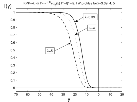
Figure 21. The TW profiles $f(y)$ of (A.14), (1.20) for $\lambda=3.39$, 4, and 5.

A.3. Non-variational KPP-problem: arbitrary $\alpha$

Indeed, with a certain extra analysis (and certain doubts), the above variational character of the problem (A.14), with $\alpha=\alpha_{0}(\lambda)$, $\lambda>0$, improves its overall mathematical quality. However, we paid so little attential to the actual possible rigorous study of (A.14), because the potential functional setting here has nothing to do with the existence of TW profiles.

To show this, consider the same problem but now with an arbitrary $\alpha\in\mathbb{R}$:

(A.21) $$u_{t}=-u_{xxxx}+\alpha u_{xxx}+u(1-u)\quad\Longrightarrow\quad-\lambda f^{\prime}=-f^{(4)}+\alpha f^{\prime\prime\prime}+f(1-f),$$

which is not variational for any $\alpha\not=\alpha_{0}(\lambda)=-2\lambda^{\frac{1}{3}}$. Note that, for $\alpha>0$, the positivity result (2.1) remains valid and the identity (2.2) now reads

(A.22) $$\textstyle{-\lambda\int(f^{\prime})^{2}=-\alpha\int(f^{\prime\prime})^{2}-\frac{1}{6}<0.}$$

It turns out that, numerically, with the full convergence up to $10^{-5}-10^{-7}$ (unlike the case $\alpha=\alpha_{0}(\lambda)$ above), we observe existence of TW profiles for both values $\alpha>0$ (Figure 22, $\lambda=1$) and $\alpha<0$ (Figure 23, $\lambda=1$). In other words, there exists a local curve of solutions originated at $\alpha=0$ with existence in some neighbourhood $\alpha\approx 0$.

For this $\lambda=1$, we have $\alpha_{0}(1)=-2$, but, for $\alpha<0$, we were not able to extend the solution for such negative $\alpha$’s. Namely, we found a “minimal” value

(A.23) $$-0.413<\alpha_{\rm min}(1)\leq-0.412\quad(\mbox{integrating on $[-50,50]$}),$$

such that, for $\alpha<\alpha_{\rm min}(1)$, there is no convergence at all, i.e., $f$ seems to be nonexistent.

Therefore, here and in [24, 25], we always did not follow any “variational temptation” to make our analysis more rigorous for some particular and specially designed KPP-problems with potential operators, and, instead, concentrated on more general aspects of the KPP-ideology and necessary and required related mathematics.

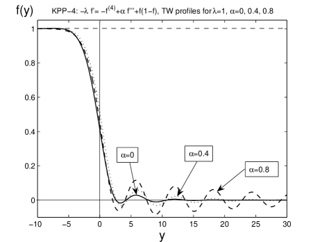
Figure 22. The TW profiles $f(y)$ of (A.21), (1.20) for $\lambda=1$ and $\alpha=0,\,0.4,\,0.8$.

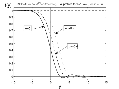
Figure 23. The TW profiles $f(y)$ of (A.21), (1.20) for $\lambda=1$ and $\alpha=0,\,-0.2,\,-0.4$.

Appendix B. A linear model: level propagation estimates from above by comparison with majorizing order-preserving integral evolution

For the semilinear KPP–$2m$ problem (1.24), (1.2), there is no the usual comparison of solutions for any $m\geq 2$. We consider the corresponding linear poly-harmonic equation

(B.1) $$u_{t}=(-1)^{m+1}D_{x}^{2m}u\quad\mbox{in}\quad\mathbb{R}\times\mathbb{R}_{+},\quad u_{0}(x)=H(-x),$$

which admits certain comparison techniques [29] by constructing a so-called majorizing order-preserving operator. This is done as follows. We first present the fundamental solution of the poly-harmonic (B.1):

(B.2) $$\textstyle{b(x,t)=t^{-\frac{1}{2m}}\,{\mathrm{e}}^{t}\,F(y),\quad y=\frac{x}{t^{1/2m}}.}$$

Substituting $b(x,t)$ into (B.1), one obtains the symmetric (even) profile $F$ as a unique solution of the linear ODE

(B.3) $$\textstyle{{\mathbf{B}}F\equiv(-1)^{m+1}F^{(2m)}+\frac{1}{2m}\,F^{\prime}y+\frac{1}{2m}\,F=0\quad{\rm in}\,\,\,\mathbb{R},\quad\int_{{\mathbb{R}}}F(y)\,{\mathrm{d}}y=1.}$$

The rescaled kernel $F(y)$ is oscillatory as $y\to\infty$ and satisfies a standard pointwise estimate [14], which is convenient to present in the form

(B.4) $$\textstyle{|F(y)|\leq D_{0}\bar{F}(y),\,\,\bar{F}(y)=\omega_{1}{\mathrm{e}}^{-d_{0}|y|^{\alpha}}>0\quad{\rm in}\,\,\,\mathbb{R},\,\,\mbox{where}\,\,\omega_{1}=\left(\int_{\mathbb{R}}{\mathrm{e}}^{-d_{0}|y|^{\alpha}}\,{\mathrm{d}}y\right)^{-1},}$$

and $D_{0}$, $d_{0}$ are some positive constants depending on $m$. The normalizing constant $\omega_{1}$ in (B.4) guarantees that the positive kernel $\bar{F}$ satisfies the standard normalization:

(B.5) $$\textstyle{\int_{\mathbb{R}}\bar{F}(y)\,{\mathrm{d}}y=1,}$$

that will allow us to use it to create below a majorizing order-preserving operator. The exponent $\alpha$ is given by

$$\textstyle{\alpha=\frac{2m}{2m-1}\in(1,2)\quad\mbox{for all}\,\,\,m\geq 2\quad(\mbox{$\alpha=2$ for $m=1$, i.e., for the Gaussian kernel}).}$$

Here $D_{0}>1$ (or $D_{0}-1>0$) is called the order deficiency of the poly-harmonic semigroup. One can see that $D$ can be made to be equal to 1, $D=1$, iff $F\geq 0$, i.e., the semigroup is order-preserving, and this happens for $m=1$ only.

Next, it is key for us to get a sharp representation of the constant $d_{0}=d_{0}(m)$. By WKBJ-type two-scale asymptotics of the solution $F(y)$ of (B.3), it is proved that $d_{0}$ is associated with the root of the algebraic equation

(B.6) $$\textstyle{(-1)^{m}a^{2m-1}=-\frac{1}{2m}.}$$

It has $2m-1$ different roots $\{a_{k}\},\,\,$ and in (B.4), we choose

(B.7) $$\textstyle{-d_{0}=\max_{k}\,\{{\rm Re}\,\alpha_{k}<0\}.}$$

For the bi-harmonic flow (B.1) with $m=2$, the rescaled kernel estimate (B.4) is

(B.8) $$|F(y)|\leq D\,\bar{F}(y)\equiv D\,\omega_{1}\,{\mathrm{e}}^{-d_{0}|y|^{4/3}}\quad\mbox{in}\quad\mathbb{R},\quad\mbox{where}\quad d_{0}=3\cdot 2^{-\frac{11}{3}}=0.2362...\,.$$

In (B.4), there appears $\bar{F}$ as the rescaled kernel of the majorizing order-preserving integral evolution equation,

(B.9) $$\textstyle{\bar{b}(x,t)=t^{\frac{1}{2m}}\,\bar{F}(y)>0,\quad y=\frac{x}{t^{1/2m}},}$$

whose solutions can be compared with those of (B.1), [29]. Obviously, for the linear KPP equations (i.e., (1.24) without the quadratic term $-u^{2}$) and the corresponding majorizing equation, the fundamental solutions are

(B.10) $$b_{*}(x,t)={\mathrm{e}}^{t}\,b(x,t)\quad\mbox{and}\quad\bar{b}_{*}(x,t)={\mathrm{e}}^{t}\,\bar{b}(x,t).$$

Consider this majorizing equation and the corresponding poly-harmonic flow

(B.11) $$\textstyle{\bar{u}(t)=\bar{b}_{*}(t)*\bar{u}_{0},\,\,\,\bar{u}_{0}(x)\geq 0\quad\mbox{and}\quad u(t)=b_{*}(t)*u_{0}\quad\mbox{for}\quad t\geq 0,}$$

with some initial data $u_{0}$ and $\bar{u}_{0}$ from the corresponding weighted $L^{2}_{\rho}(\mathbb{R})$ ($\rho={\mathrm{e}}^{-a_{0}|x|^{\alpha}}$, $a_{0}\in(0,2d_{0}]$) space of correctedness. Subtracting these two and using (B.4) yield

(B.12) $$\bar{u}(t)-u(t)= \bar{b}_{*}(t)*\bar{u}_{0}-b_{*}(t)*u_{0}\geq\bar{b}_{*}(t)*\bar{u}_{0}-|b_{*}(t)|*|u_{0}|$$

$$\geq \bar{b}_{*}(t)*\bar{u}_{0}-D_{0}\bar{b}_{*}(t)*|u_{0}|\geq{\mathrm{e}}^{t}\,\bar{b}(t)*(\bar{u}_{0}-D_{0}|u_{0}|),$$

whence the following result:

Proposition B.2.

$($Comparison$)$ There is comparison of solutions of $\eqref{maj1}$, i.e.,

(B.13) $$u(x,t)\leq\bar{u}(x,t)\quad\mbox{in}\quad\mathbb{R}\times\mathbb{R}_{+}\,\,\,\mbox{for majorizing data}\,\,\,\bar{u}_{0}(x)=D_{0}|u_{0}(x)|\geq 0\,\,\mbox{in}\,\,\mathbb{R}.$$

Consider now the majorizing solution

(B.14) $$\bar{u}(x,t)=m_{0}{\mathrm{e}}^{t}\,\bar{b}(x,t)\,\,\,\mbox{corresponding to Dirac's delta function}\,\,\,\bar{u}_{0}(x)=m_{0}\delta(x),$$

where $m_{0}$ is a sufficiently large constant to be estimated. We now treat (B.14) as a solution of the boundary value problem in $\mathbb{R}_{+}\times\mathbb{R}_{+}$ with the symmetry conditions at the boundary point $x=0$ (of course, at the same time, this is a solution of the Cauchy problem):

(B.15) $$u_{x}(0,t)=u_{xxx}(0,t)=...=D_{x}^{2m-1}u(0,t)=0\quad\mbox{for}\quad t\geq 0.$$

We now choose $m_{0}>0$ so large that

(B.16) $$D_{0}u(0,t)\leq\bar{u}(0,t)\quad\mbox{for}\quad t\geq 0.$$

Then the same argument of majorizing comparison guarantees that

(B.17) $$u(x,t)\leq\bar{u}(x,t)\quad\mbox{in}\quad\mathbb{R}_{+}\times\mathbb{R}_{+}.$$

This inequality allows to estimate the $\frac{1}{2}$-level propagation (1.10) for $u(x,t)$: indeed, $x_{f}(t)\leq\bar{x}_{f}(t)$, where $\bar{x}_{f}(t)$ solves

(B.18) $$\textstyle{{\mathrm{e}}^{t}\,t^{-\frac{1}{2m}}\bar{F}\big{(}\frac{\bar{x}_{f}(t)}{t^{1/2m}}\big{)}=\frac{1}{2},\quad\mbox{or}\quad\bar{F}\big{(}\frac{\bar{x}_{f}(t)}{t^{1/2m}}\big{)}=t^{\frac{1}{2m}}\,{\mathrm{e}}^{-t}\to 0\quad\mbox{as}\quad t\to\infty.}$$

Using (B.4), we finally obtain the estimate

(B.19) $$\textstyle{x_{f}(t)\leq\bar{x}_{f}(t)=d_{0}^{-\frac{2m-1}{2m}}t-\frac{2m-1}{(2m)^{2}}\,d_{0}^{-\frac{2m-1}{2m}}\log t(1+o(1)),\quad t\to\infty.}$$

Therefore, formally (without a proof, since comparison was not performed for full nonlinear KPP–problems; see also comments below), we have the following bound for the minimal speed:

(B.20) $$\lambda_{0}\leq\lambda_{*}=d_{0}^{-\frac{2m-1}{2m}}\quad\mbox{and}\quad\lambda_{0}\leq\lambda_{*}=3^{-\frac{3}{4}}\cdot 2^{\frac{11}{4}}=2.9512...\quad\mbox{for}\quad m=2.$$

If this minimal speed actually takes place, then (B.19) gives a lower estimate of $k=k(m)$:

(B.21) $$\textstyle{\lambda_{0}=\lambda_{*}:\,\,\,k\geq k_{*}=\frac{2m-1}{(2m)^{2}}\,d_{0}^{-\frac{2m-1}{2m}},\,\,\,k\geq k_{*}=3^{\frac{1}{4}}\cdot 2^{-\frac{5}{4}}=0.5533...\quad\mbox{for}\quad m=2.}$$

Finally, it is worth mentioning that the estimates (B.20) and (B.21) make more sense for the KPP-like problems for the semilinear majorizing order-preserving integral, “pseudo-differential” evolution equation (recall again that it is not a flow, with no a semigroup and $t$-translational invariance available)

(B.22) $$\textstyle{\bar{u}(t)=\bar{b}(t)*\bar{u}_{0}+\int\limits_{0}^{t}\bar{b}(t-s)*u(s)(1-u(s))\,{\mathrm{d}}s,}$$

which is far away from semigroups for the original KPP–problems for higher-order differential operators.

Remark: on comparison in semilinear KPP–$2m$ problem. For $m=1$, there is no problem, since $-u^{2}\leq 0$, so that $\bar{u}(x,t)$ is always a super-solution.

Let $m\geq 2$, then the integral equation via the Duhamel principle reads

(B.23) $$\textstyle{u(t)={\mathrm{e}}^{t}b(t)*u_{0}-\int\limits_{0}^{t}b(t-s)*({\mathrm{e}}^{s}u^{2}(s))\,{\mathrm{d}s}.}$$

Therefore, the final inequality similar to (B.12) now contains an extra term:

(B.24) $$\textstyle{\bar{u}(t)-u(t)\geq{\mathrm{e}}^{t}\,\bar{b}(t)*(\bar{u}_{0}-D_{0}|u_{0}|)+\int\limits_{0}^{t}b(t-s)*({\mathrm{e}}^{s}u^{2}(s))\,{\mathrm{d}s}\equiv J_{1}(t)+J_{2}(t),}$$

where $J_{1}(t)\geq 0$ by Proposition B.2. However, since $b(x,t)$ changes sign, in general, we cannot control the positive sign of the last term (though $u^{2}\geq 0$) for absolutely arbitrary solutions. Thus, any “unconventional” comparison results are not available, and this is well known for higher-order parabolic flows.

But we recall that we need a proper estimate above for $t\gg 1$, where our solution is assumed to be approaching (with a shift) to a TW, i.e., we may assume that

(B.25) $$u(x,t)\to f(x-x_{f}(t)),\,\,\,x_{f}(t)=\lambda_{0}t-g(t),\quad\mbox{uniformly in $x\in\mathbb{R}$ as}\quad t\to+\infty.$$

Moreover, we need such an upper estimate on a level set $\{u(x,t)=\frac{1}{2}\}$ for $t\gg 1$. Therefore, the second term on the right-hand side of (B.24) can be arbitrarily sharply approximated by

(B.26) $$\textstyle{J_{2}(t)\sim\int\limits_{0}^{t}b(t-s)*({\mathrm{e}}^{s}f^{2}(\cdot))\,{\mathrm{d}s}\quad\mbox{as}\quad t\to+\infty,}$$

and this approximation gets sharper as $t$ increases. Bearing in mind rather smooth TW profiles $f(y)$ (cf. Figures 1, 2, 5, etc.), representing an “almost monotone” (with just slightly oscillating tails at $y\to\pm\infty$) heteroclinic path of equilibria 1 and 0, and overall “dominant positivity” of the fundamental solution $b(x,t)$ ($\int b(x,t)\,{\mathrm{d}}x\equiv+1$), there is a sufficient probability that

(B.27) $$J_{2}(x,t)>0\quad\mbox{for}\quad t\gg 1\quad\mbox{and for large enough $x$,}$$

at least in an “a.a. sense”, in a natural way. If (B.27) is true, then, by (B.24), the front propagation estimates (B.19)–(B.21) actually hold.

The positivity (B.27) of the integral in (B.26) deserves further analytic study, though it is very difficult, since the TW profiles are not known explicitly. On the other hand, let us note that the asymptotic positivity (B.27) on the front curve $\{x=x_{f}(t)\}$ can be studied numerically, but, without any doubt, we believe that it actually takes place justifying the above TW speed and $k$-estimates.

References

- [1] G.I. Barenblatt, Similarity, Self-Similarity, Intermediate Asymptotics, Consultant Bureau, New York, 1978.
- [2] A.L. Bertozzi, A. Münch, M. Shearer, and K. Zumbrun, Stability of compressive and undercompressive thin film travelling waves, Euro J. Appl. Math., 12 (2001), 253–291.
- [3] C.J. Budd, V.A. Galaktionov, and J.F. Williams, Self-similar blow-up in higher-order semilinear parabolic equations, SIAM J. Appl. Math., 65 (2004), 1775–1809.
- [4] M. Bramson, Convergence of solutions of the Kolmogorov equation to travelling waves, Memoirs of Amer. Math. Soc., 44 (1983), 1–190.
- [5] H. Brezis, L.A. Peletier, and D. Terman, A very singular solution of the heat equation with absorption, Arch. Ration. Mech. Anal., 95 (1986), 185–209.
- [6] J. Busca, M.A. Jendoubi, and P. Polác̆ik, Convergence to equilibrium for semilinear parabolic problems, Commun. Part. Differ. Equat., 27 (2002), 1793-1814.
- [7] R. Chill, On the Łojasiewicz–Simon gradient inequality, J. Funct. Anal., 201 (2003), 572-601.
- [8] E.A. Coddington and N. Levinson, Theory of Ordinary Differential Equations, McGraw-Hill Book Company, Inc., New York/London, 1955.
- [9] P. Collet and J.-P. Eckmann, Instabilities and Fronts in Extended Systems, Pinceton Univ. Press, Princeton, NJ, 1990.
- [10] A.-C. Coulon and J.-M. Roquejoffre, Transition between linear and exponential propagation in Fisher-KPP type reaction-diffusion equations, (arXiv:1111.0408).
- [11] U. Ebert and W. van Saarloos, Front propagation into unstable fronts: universal algebraic convergence towards uniformly translating pulled fronts, Physica D, 46 (2000), 1–99.
- [12] Yu.V. Egorov, V.A. Galaktionov, V.A. Kondratiev, and S.I. Pohozaev, On the necessary conditions of existence to a quasilinear inequality in the half-space, Comptes Rendus Acad. Sci. Paris, 330 (2000), 93–98.
- [13] Yu.V. Egorov, V.A. Galaktionov, V.A. Kondratiev, and S.I. Pohozaev, Global solutions of higher-order semilinear parabolic equations in the supercritical range, Adv. Differ. Equat., 9 (2004), 1009–1038.
- [14] S.D. Eidelman, Parabolic Systems, North-Holland Publ. Comp., Amsterdam/London, 1969.
- [15] J.D. Evans, V.A. Galaktionov, and J.R. King, Source-type solutions of the fourth-order unstable thin film equation, Euro J. Appl. Math., 18 (2007), 273–321.
- [16] J.D. Evans, V.A. Galaktionov, and J.F. Williams, Blow-up and global asymptotics of the limit unstable Cahn-Hilliard equation, SIAM J. Math. Anal., 38 (2006), 64–102.
- [17] E. Fereisl, F. Issard-Roch, and H. Petzeltova, A non-smooth vedrsion of the Lojasiewicz–Simon theorem with applications to non-local phase-field systems, J. Differ. Equat., 199 (2004), 1-21.
- [18] A. Friedman, On the regularity of the solutions of nonlinear elliptic and parabolic systems of partial differential equations, J. Math. Mech., 7 (1958), 43–59.
- [19] V.A. Galaktionov, Comments on the magic exponent in Kolmogorov-Petrovskii-Piskunov problem. A discussion proposal (to the Reaction–Diffusion and Probability Groups, Dept. Math. Sci., University of Bath), December 1995, unpublished.
- [20] V.A. Galaktionov, On a spectrum of blow-up patterns for a higher-order semilinear parabolic equation, Proc. Royal Soc. London A, 457 (2001), 1–21.
- [21] V.A. Galaktionov, Critical global asymptotics in higher-order semilinear parabolic equations, Int. J. Math. Math. Sci., 60 (2003), 3809–3825.
- [22] V.A. Galaktionov, Geometric Sturmian Theory of Nonlinear Parabolic Equations and Applications, ChapmanHall/CRC, Boca Raton, Florida, 2004.
- [23] V.A. Galaktionov, On interfaces and oscillatory solutions of higher-order semilinear parabolic equations with non-Lipschitz nonlinearities, Stud. Appl. Math., 117 (2006), 353–389.
- [24] V.A. Galaktionov, Towards the KPP–problem and –front shift for higher-order nonlinear PDEs II. Quasilinear bi- and tri-harmonic equations, in preparation (shortly, to appear in arXiv.org).
- [25] V.A. Galaktionov, Towards the KPP–problem and –front shift for higher-order nonlinear PDEs III. Dispersion and hyperbolic equations, in preparation (shortly, to appear in arXiv.org).
- [26] V.A. Galaktionov, S.P. Kurdyumov, and A.A. Samarskii, On asymptotic “eigenfunctions” of the Cauchy problem for a nonlinear parabolic equation, Mat. Sbornik, 126 (1985), 435–472 (in Russian); English translation: Math. USSR Sbornik, 54 (1986), 421–455.
- [27] V.A. Galaktionov, E. Mitidieri, and S.I. Pohozaev, Variational approach to complicated similarity solutions of higher-order nonlinear evolution equations of parabolic, hyperbolic, and nonlinear dispersion types, In: Sobolev Spaces in Mathematics. II, Appl. Anal. and Part. Differ. Equat., Series: Int. Math. Ser., Vol. 9, V. Maz’ya Ed., Springer, 2009 (an earlier preprint: arXiv:0902.1425).
- [28] V.A. Galaktionov, E. Mitidieri, and S.I. Pohozaev, Variational approach to complicated similarity solutions of higher-order nonlinear PDEs. II, Nonl. Anal.: RWA, 12 (2011), 2435–2466 (arXiv:1103.2643).
- [29] V.A. Galaktionov and S.I. Pohozaev, Existence and blow-up for higher-order semilinear parabolic equations: majorizing order-preserving operators, Indiana Univ. Math. J., 51 (2002), 1321–1338.
- [30] V.A. Galaktionov, S.I. Pohozaev, and A.E. Shishkov On convergence in smooth gradient systems with branching of equilibria, Mat. Sbornik, 198 (2007), 817–838 (arXiv:0902.0286).
- [31] V.A. Galaktionov and J.L. Vazquez, Asymptotic behaviour of nonlinear parabolic equations with critical exponents. A dynamical systems approach, J. Funct. Anal., 100 (1991), 435–462.
- [32] V.A. Galaktionov and J.L. Vazquez, Extinction for a quasilinear heat equation with absorption II. A dynamical systems approach, Comm. Partial Differ. Equat., 19 (1994), 1107–1137.
- [33] V.A. Galaktionov and J.L. Vazquez, A Stability Technique for Evolution Partial Differential Equations. A Dynamical Systems Approach, Birkhäuser, Boston/Berlin, 2004.
- [34] J. Gärtner, Location of wave front for the multidimensional K-P-P equation and brownian first exit densities, Math. Nachr., 105 (1982), 317–351.
- [35] H. Gao and C. Liu, Instability of travelling waves of the convective-diffusive Cahn–Hilliard equation, Chaos, Solit. Fract., 20 (2004), 253–258.
- [36] A. Gmira and L. Véron, Large time behaviour of solutions of a semilinear problem in , J. Differ. Equat., 53 (1984), 258–276.
- [37] J.K. Hale and G. Raugel, Convergence in gradient-like systems with applications to PDE, Z. angew. Math. Phys., 43 (1992), 63-124.
- [38] F. Hamel and L. Roques, Fast propagation for KPP equations with slow decaying initial conditions, J. Differ. Equat., bf 249 (2010), 1726–1745. (arXiv:0906.3164).
- [39] A. Haraux and M.A. Jendoubi, Decay estimates to equilibrium for some evolution equations with an analytic nonlinearity, Asympt. Anal., 26 (2001), 21–36.
- [40] A. Haraux and M.A. Jendoubi, The Łojasiewicz gradient inequality in the infinite-dimensional Hilbert space framework, J. Funct. Anal., 260 (2011), 2826–2842.
- [41] W.D. Kalies, J. Kwapisz, J.B. VandenBerg, and R.C.A.M. VanderVorst, Homotopy classes for stable periodic and chaotic patterns in fourth-order Hamiltonian systems, Commun. Math. Phys., 214 (2000), 573–592.
- [42] S. Kamin (Kamenomostskaya), The asymptotic behaviour of the solution to the filtration equation, Israel J. Math., 14 (1973), 76–87.
- [43] S. Kamin and L.A. Peletier, Large time behaviour of solutions of the heat equation with absorption, Ann. Sc. Norm. Pisa (4), 12 (1984), 393–408.
- [44] A.N. Kolmogorov, The local structure of turbulence in incompressible viscous fluids at very large Reynolds numbers, Dokl. Akad. Nauk. SSSR, 30 (1941), 301–305.
- [45] A.N. Kolmogorov, I.G. Petrovskii, and N.S. Piskunov, Study of the diffusion equation with growth of the quantity of matter and its application to a biological problem, Byull. Moskov. Gos. Univ., Sect. A, 1 (1937), 1–26. English. transl. In: Dynamics of Curved Fronts, P. Pelcé, Ed., Acad. Press, Inc., New York, 1988, pp. 105–130.
- [46] Z. Li and C. Liu, On the nonlinear instability of travelling waves for a sixth order parabolic equation, Abstr. Appl. Anal., to appear.
- [47] A. Lunardi, Analytic Semigroups and Optimal Regularity in Parabolic Problems, Birkhäuser, Basel/Berlin, 1995.
- [48] M.A. Naimark, Linear Differential Operators, Part 1, Frederick Ungar Publ. Co., New York, 1967.
- [49] A.M. Obukhov, On the distribution of energy in the spectrum of a turbulent flow, Dokl. Akad Nauk SSSR, 32 (1941), 22–24.
- [50] L.A. Peletier and W.C. Troy, Spatial Patterns. Higher Order Models in Physics and Mechanics, Birkhäuser, Boston/Berlin, 2001.
- [51] A.A. Samarskii, V.A. Galaktionov, S.P. Kurdyumov, and A.P. Mikhailov, Blow-up in Quasilinear Parabolic Equations, Walter de Gruyter, Berlin/New York, 1995.
- [52] W. Strauss, A. Walter, and G. Wang, Instability of travelling waves of the Cahn–Hilliard equation, In: Front. Math. Anal. Numer. Meth., World Sci. Publ., River Edge, NJ, 2004, pp. 253-266.
- [53] J.B. Van Den Berg and R.C. Vandervorst, Stable patterns for fourth-order parabolic equations, Duke Math. J., 115 (2002), 513–558.
- [54] V. Vergara, Convergence to steady states of solutions to nonlinear integral evolution equations, Calc. Var., 40 (2011), 319–334.
- [55] E. Yanagida, Irregular behaviour of solutions for Fisher’s equation, J. Dyn. Differ. Equat., 19 (2007), 895–914.
- [56] H. Yassine, Asymptotic behaviour and decay rate estimates for a class of semilinear evolution equations of mixed order, Nonl. Anal., 74 (2011), 2309–2326.
- [57] T.I. Zelenyak, Stabilization of solutions of boundary value problems for a second order parabolic equation with one space variable, Differ. Equat., 4 (1968), 17–22.