Effects of Compton Cooling on Outflow in a Two Component Accretion Flow around a Black Hole: Results of a Coupled Monte Carlo-TVD Simulation
Abstract
We wish to investigate the effects of cooling of the Compton cloud on the outflow formation rate in an accretion disk around a black hole. We carry out a time dependent numerical simulation where both the hydrodynamics and the radiative transfer processes are coupled together. We consider a two-component accretion flow in which the Keplerian disk is immersed into an accreting low-angular momentum flow (halo) around a black hole. The soft photons which originate from the Keplerian disk are inverse-Comptonized by the electrons in the halo and the region between the centrifugal pressure supported shocks and the horizon. We run several cases by changing the rate of the Keplerian disk and see the effects on the shock location and properties of the outflow and the spectrum. We show that as a result of Comptonization of the Compton cloud, the cloud becomes cooler with the increase in the Keplerian disk rate. As the resultant thermal pressure is reduced, the post-shock region collapses and the outflow rate is also reduced. Since the hard radiation is produced from the post-shock region, and the spectral slope increases with the reduction of the electron temperature, the cooling produces softer spectrum. We thus find a direct correlation between the spectral states and the outflow rates of an accreting black hole.
e-mail: himadri@bose.res.in
1 Introduction
It is generally believed that the outflows and jets in a compact binary system containing black holes originate from the disk itself. There are several hydrodynamical models of the formation of outflows from the disks ranging from the twin-exhaust model of Blandford & Rees [1974], to the self-similar models of Blandford & Payne [1982] and Blandford & Begelman [1999]. Assuming that the outflows are transonic in nature, Fukue [1983] and Chakrabarti [1986] computed the velocity distribution without and with rotational motion in the flow and showed that the flow could become supersonic close to the black hole. Camenzind and his group extensively worked on the magnetized jets and showed that the acceleration and collimation of the jets could be achieved [e.g., Appl & Camenzind, 1993]. In a subsequent two component transonic flow model, Chakrabarti & Titarchuk [1995] pointed out that the jets could be formed only from the inner part of the disk, which is also known as the Centrifugal pressure dominated boundary layer or CENBOL. The CENBOL is the Compton cloud in a two component flow and is the region between the accretion shock formed by centrifugal barrier at a few tens of Schwarzschild radii () and the inner sonic point located at . If this region remains hot, it would emit hard radiation and the spectrum of the disk would be hard. The reverse is true if the Compton cloud (CENBOL) is cooled down and the spectrum would be soft.
While the general picture of the outflow formation is thus understood and even corroborated by the radio observation of the base of the powerful jet, such as in M87 [Junor et al., 1999] that the base of the jet is only a few tens of , a major question still remained: what fraction of the matter is driven out from the disk and what are the flow parameters on which this fraction depends? In a numerical simulation using smoothed particle hydrodynamics (SPH), Molteni et al. [1994], showed that the outflow rates from an inviscid accretion flow strongly depends on the outward centrifugal force and 15-20 percent matter can be driven out of the disk. Chakrabarti [1998, 1999] and Chattopadhyay et al. [2004] estimated the ratio of the outflow rate to inflow rate analytically and found that the shock strength determines the ratio. For very strong and very weak shocks, the outflow rates are very small, while for the shocks of intermediate strength, the outflow rate is significant. These works were further refined by Singh & Chakrabarti [2011] who studied the outflow rates self-consistently by modifying the Rankine-Hugoniot relations in presence of both energy and mass dissipation. These authors showed that with the increase of dissipation of energy in the flow, the outflow rate is greatly reduced. This is in line with the recent observations Fender et al. [2010] that the spectrally soft states have less outflows.
In the present paper, we concentrate on the numerical simulations of accretion flows around black holes which are coupled to radiative transfer. While computing the time variation of the velocity components, density and temperature we also compute the temporal dependence of the spectral properties. As a result, not only we compute the outflow properties, we correlate them with the spectral properties – a first in this subject. Not surprisingly, we find that whenever the Compton cloud or the CENBOL is cooled down and the spectrum becomes softer, the flow, originating from CENBOL, losses its drive and the outflow rate is greatly reduced.
Carrying out hydrodynamic simulations around black holes is not new. Hawley et al. [1984] pioneered the study of accretion flows around black holes. Subsequent work of Hawley & Balbus [1992] with magnetized flow indicated how the angular momentum may be transported and matter may accrete efficiently. These works used finite difference method. Igumenshchev et al. [1996] studied two-dimensional flows but concentrated only the inner region of the disk, namely, the region less than . Their main interest was to study the transonic nature of the flow outside the horizon. Ryu et al. [1995] studied unstable shocks in an inviscid flow, while Ryu et al. [1997] studied the oscillations of the centrifugal pressure driven shocks when Rankine-Hugoniot relations are not satisfied. In a significant development which connects the time dependence of accretion flows with quasi-periodic oscillations, Molteni et al. [1996] suggested that the shocks can oscillate whenever the cooling time scale roughly matches with the infall timescale in the post-shock region. Although only the bremsstrahlung cooling was used, this work provides a natural explanation of the quasi-periodic oscillations or QPOs which are observed in black hole candidates. Lanzafame et al. [1998] carried out the SPH simulation in a region with a radial extent of in two dimensions and concentrated on the shock formation. They demonstrated that a high viscosity can remove the shock from an accretion flow [see also, Giri & Chakrabarti, 2012]. Igumenshchev et al. [1998] used the finite difference method and allowed the heat generated by viscosity to be radiated away or absorbed totally. The computational box was up to , but the outer boundary condition was that of a near Keplerian flow having no radial velocity. The inner boundary was kept at . Thus the possibility of having a shock or the inner sonic point was excluded. The detailed radiative transfer, especially Comptonization was not included. To our knowledge, ours is a first step to include Comptonization coupled to hydrodynamic simulations where both the sources of soft photons (Keplerian disk) and the hot electrons (low angular momentum flows) are included. Evidence of such a two-component flow is present in many of the observations of the black hole candidates [Smith et al., 2001, 2002, Soria et al., 2001, Wu et al., 2002].
In the next Section, we discuss the geometry of the soft photon source and the Compton cloud in our Monte Carlo simulations. The variation of the thermodynamic quantities and other vital parameters are obtained inside the Keplerian disk and the Compton cloud which are required for the Monte Carlo simulations. In §3, we describe the simulation procedure and in §4, we present the results of our simulations. Finally, in §5, we make concluding remarks.
2 Geometry of the electron cloud and the soft photon source
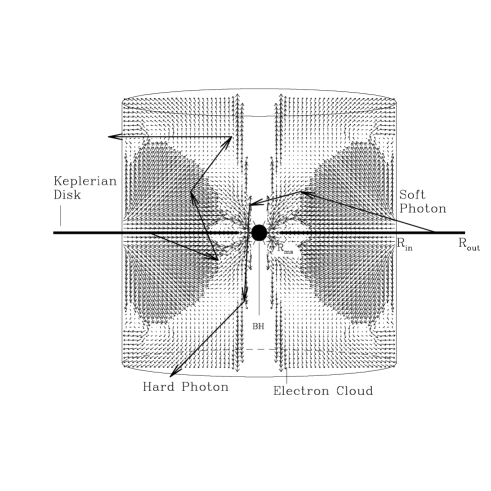
In Figure 1, we present the cartoon diagram of our simulation set up for the Compton cloud with a specific angular momentum (angular momentum per unit mass) . The sub-Keplerian matter is injected from the outer boundary at (). The Keplerian disk resides at the equatorial plane of the cloud. The outer edge of this disk is located at and it extends up to the marginally stable orbit . At the centre, a black hole of mass is located. The soft photons emerging out of the Keplerian disk are intercepted and reprocessed via Compton or inverse-Compton scattering by the sub-Keplerian matter. An injected photon may undergo no scattering at all or a single or multiple with the hot electrons in between its emergence from the Keplerian disk and its escape from the halo. The photons which enter the black hole are absorbed.
2.1 Distribution of temperature and density inside the Compton cloud
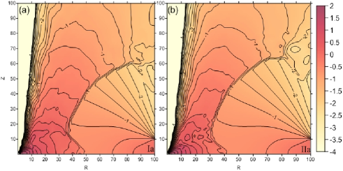
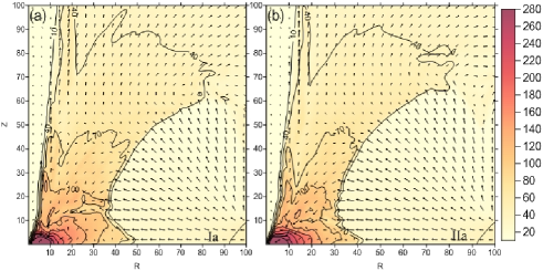
A realistic accretion disk is expected to be three-dimensional. Assuming axisymmetry, we have calculated the flow dynamics using a finite difference method which uses the principle of total variation diminishing (TVD) to carry out hydrodynamic simulations [see, Ryu et al., 1997, Giri et al., 2010, and references therein;]. At each time step, we carry out Monte Carlo simulation to obtain the cooling/heating due to Comptonization. We incorporate the cooling/heating of each grid while executing the next time step of hydrodynamic simulation. The numerical simulation for the two-dimensional flow has been carried out with cells in a box. We choose the units in a way that the outer boundary () is unity and the matter density at the outer boundary is also normalized to unity. We assume the black hole to be non-rotating and we use the pseudo-Newtonian potential [Paczyński & Wiita, 1980] to calculate the flow geometry around a black hole (Here, is in the unit of Schwarzschild radius .). Velocities and specific angular momenta are measured in units of , the velocity of light and respectively. In Figures (2) and (3) we show the snapshots of the density and temperature (in keV) profiles obtained in a steady state purely from the hydrodynamic simulation. For both the angular momenta cases, we find the presence of two shocks in the accretion flow in the steady state: one paraboloidal shock and the other oblate spheroidal shock near the equatorial plane [Molteni et al., 1996]. Due to the increased centrifugal barrier, the shock forms at a larger radius for the case .
2.2 Properties of the Keplerian disk
In our simulation, the soft photons are produced from a Keplerian disk, the inner and the outer edges of which have been kept fixed at the marginally stable orbit , and at respectively. The source of the soft photons has a multi-color blackbody spectrum coming from a standard [Shakura & Sunyaev, 1973, hereafter SS73] Keplerian disk. The disk is assumed to be optically thick and the opacity due to free-free absorption is assumed to be more important than the opacity due to scattering. The emission is black body type with the local surface temperature (SS73):
| (1) |
The total number of photons emitted from the disk surface is obtained by integrating over all frequencies () and is given by,
| (2) |
The disk between radius to produces number of soft photons.
| (3) |
where, is the half height of the disk given by:
| (4) |
In the Monte Carlo simulation, we incorporated the directional effects of photons coming out of the Keplerian disk with the maximum number of photons emitted in the -direction and minimum number of photons are generated along the plane of the disk. Thus, in the absence of photon bending effects, the disk is invisible as seen edge on. The position of each emerging photon is randomized using the distribution function (Eq. 3). In the above equations, the mass of the black hole is measured in units of the mass of the Sun (), the disk accretion rate is in units of gm/s. We chose in the rest of the paper. Generally, we follow Ghosh et al. [2009, 2010] while modeling the soft photon source.
3 Simulation Procedure
For a particular simulation, we use the Keplerian disk rate () and the sub-Keplerian halo rate () as parameters. The specific energy () and the specific angular momentum () determines the hydrodynamics (shock location, number density and velocity variations etc.) and the thermal properties of the sub-Keplerian matter. We assume the absorbing boundary condition at since any inward pointing photon at that radius would be sucked into the black hole.
3.1 Details of the hydrodynamic simulation code
To model the initial injection of matter, we consider an axisymmetric flow of gas in the pseudo-Newtonian gravitational field of a black hole of mass located at the centre in the cylindrical coordinates . We assume that at infinity, the gas pressure is negligible and the energy per unit mass vanishes. We also assume that the gravitational field of the black hole can be described by Paczyński & Wiita [1980] potential,
where, . We assume a polytropic equation of state for the accreting (or, outflowing) matter, , where, and are the isotropic pressure and the matter density respectively, is the adiabatic index (assumed to be constant throughout the flow, and is related to the polytropic index by ) and is related to the specific entropy of the flow . is not constant but is allowed to vary due to radiative processes. The details of the code is described in Molteni et al. [1996] and in Giri et al. [2010].
Our computational box occupies one quadrant of the R-z plane with and . The incoming gas enters the box through the outer boundary, located at . We have chosen the density of the incoming gas for convenience. In the absence of self-gravity and cooling, the density is scaled out, rendering the simulation results valid for any accretion rate. As we are considering only energy flows while keeping the boundary of the numerical grid at a finite distance, we need the sound speed (i.e., temperature) of the flow and the incoming velocity at the boundary points. In order to mimic the horizon of the black hole at the Schwarzschild radius, we place an absorbing inner boundary at , inside which all material is completely absorbed into the black hole. For the background matter (required to avoid division by zero) we use a stationary gas with density and sound speed (or temperature) the same as that of the incoming gas. Hence the incoming matter has a pressure times larger than that of the background matter. All the calculations were performed with cells, so each grid has a size of in units of the Schwarzschild radius.
3.2 Details of the radiative transfer code
To begin a Monte-Carlo simulation, we generate photons from the Keplerian disk with randomized locations as mentioned in the earlier section. The energy of the soft photons at radiation temperature is calculated using the Planck’s distribution formula, where the number density of photons () having an energy is expressed by Pozdnyakov et al. [1983],
| (5) |
where, and , the Riemann zeta function. Using another set of random numbers we obtained the direction of the injected photon and with yet another random number we obtained a target optical depth at which the scattering takes place. The photon was followed within the electron cloud till the optical depth () reached . The increase in optical depth () during its traveling of a path of length inside the electron cloud is given by: , where is the electron number density.
The total scattering cross section is given by Klein-Nishina formula:
| (6) |
where, is given by,
| (7) |
is the classical electron radius and is the mass of the electron.
We have assumed here that a photon of energy and momentum is scattered by an electron of energy and momentum , with and . At this point, a scattering is allowed to take place. The photon selects an electron and the energy exchange is computed using the Compton or inverse Compton scattering formula. The electrons are assumed to obey relativistic Maxwell distribution inside the Compton cloud. The number of Maxwellian electrons having momentum between to is expressed by,
| (8) |
In passing we wish to note that in the region of our interest (i.e. ) and for stellar mass black holes, the free-free absorption and/or emission is inefficient [e.g., Narayan & Yi, 1995, Das & Chattopadhyay, 2008]. This can be shown as follows:
The Compton cooling rate for a thermal distribution of nonrelativistic electrons of number density and temperature is [Rybicki & Lightman, 1979, Niedzwiecki et al., 1997]: , ( is the radiation energy density, is the Thomson scattering cross-section, is the speed of light, is the mass of the electron and is the Boltzmann constant) while the bremsstrahlung cooling rate is given by . Using usual formulas for and , the ratio of the cooling rates turns out to be
To compute , assume, and . For (pre-shock), K, /cc, and for (post-shock), K, /cc . Thus both in the pre-shock and the post-shock regions, Comptonization is much more effective compared to bremsstrahlung. In the simulation we ignore bremsstrahlung. Of course, this conclusion depends on the mass of the black hole and should be considered for super-massive black holes, for instance.
3.2.1 Calculation of energy reduction using Monte Carlo code:
We divide the Keplerian disk in different annuli of width . Each annulus having mean radius is characterized by its average temperature . The total number of photons emitted from the disk surface of each annulus can be calculated using Eq. 3. This total number comes out to be per second for . In reality, one cannot inject these many number of photons in Monte Carlo simulation because of the limitation of computation time. So we replace this large number of photons by a lower number of bundles of photons, say, and calculate a weightage factor
Clearly, from annulus to annulus, the number of photons in a bundle will vary. This is computed from the standard disk model and is used to compute the change of energy by Comptonization. When the injected photon is inverse-Comptonized (or, Comptonized) by an electron in a volume element of size , we assume that number of photons has suffered similar scattering with the electrons inside the volume element . If the energy loss (gain) per electron in this scattering is , we multiply this amount by and distribute this loss (gain) among all the electrons inside that particular volume element. This is continued for all the bundles of photons and the revised energy distribution is obtained.
3.2.2 Computation of the temperature distribution after cooling
Since the hydrogen plasma considered here is ultra-relativistic ( throughout the hydrodynamic simulation), thermal energy per particle is where is Boltzmann constant, is the temperature of the particle. The electrons are cooled by the inverse-Comptonization of the soft photons emitted from the Keplerian disk. The protons are cooled because of the Coulomb coupling with the electrons. Total number of electrons inside any box with the centre at location is given by,
| (9) |
where, is the electron number density at location, and and represent the grid size along and directions respectively. So the total thermal energy in any box is given by where is the temperature at grid. We calculate the total energy loss (gain) of electrons inside the box according to what is presented above and subtract that amount to get the new temperature of the electrons inside that box as
| (10) |
3.3 Coupling procedure
The hydrodynamic and the radiative transfer codes are coupled together following the same procedure as in Ghosh et al. [2011]. Once a quasi steady state is achieved using the non-radiative hydro-code, we compute the radiation spectrum using the Monte Carlo code. This is the first approximation of the spectrum. To include the cooling in the coupled code, we follow these steps: (i) We calculate the velocity, density and temperature profiles of the electron cloud from the output of the hydro-code. (ii) Using the Monte Carlo code we calculate the spectrum. (iii) Electrons are cooled (heated up) by the inverse-Compton (Compton) scattering. We calculate the amount of heat loss (gain) by the electrons and its new temperature and energy distributions and (iv) Taking the new temperature and energy profiles as initial condition, we run the hydro-code for a period of time much shorter (by a factor of ) than the cooling or infall time scale. Subsequently, we repeat the steps (i-iv). In this way, we see how the spectrum is modified and eventually converged as the iterations proceed.
Earlier we mentioned that we injected bundles. Before the choice of was made, we varied from to and conducted a series of runs to ensure that our final result does not suffer from any statistical effects. Figure 4 shows the average electron temperature of the cloud when was varied. There is a clear convergence in our result for . Thus, our choice of is quite safe.
All the simulations are carried out assuming a stellar mass black hole . The procedures remain equally valid for massive/super-massive black holes though free-free absorption/emission may have to be included. We carry out the simulations for more than dynamical time-scales. In reality, this corresponds to a few seconds in physical units for the chosen gridsize.
4 Results and Discussions
| Table 1: Parameters used for the simulations. | |||
| Case | |||
| Ia | 0.0021, 1.76 | 1.0 | No Disk |
| Ib | 0.0021, 1.76 | 1.0 | 0.5 |
| Ic | 0.0021, 1.76 | 1.0 | 1.0 |
| Id | 0.0021, 1.76 | 1.0 | 2.0 |
| IIa | 0.0021, 1.73 | 1.0 | No Disk |
| IIb | 0.0021, 1.73 | 1.0 | 0.5 |
| IIc | 0.0021, 1.73 | 1.0 | 1.0 |
| IId | 0.0021, 1.73 | 1.0 | 2.0 |
In Table 1, we list various Cases with all the simulation parameters used in the present paper. The specific energy () and specific angular momentum () of the sub-Keplerian halo are given in Column 2. Columns 3 and 4 give the halo () and the disk () accretion rates. The corresponding cases are marked in Column 1. In Cases Ia and IIa, no Keplerian disk was placed in the equatorial plane of the halo. These are non-radiative hydrodynamical simulations and no Compton cooing is included. To show the effects of Compton cooling on the hydrodynamics of the flow, the Cases I(b-d) and II(b-d) are run for the same time as the Cases Ia and IIa.
4.1 Properties of the shocks in presence of cooling
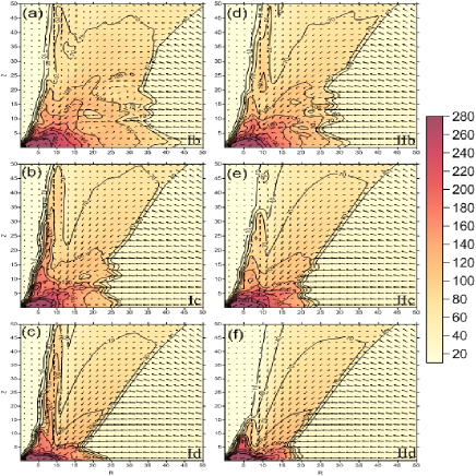
In Figures 5(a) and 5(b), we present the time variation of the shock location (in units of ) for various Cases (marked on each curve) given in Table 1. All the solutions exhibit oscillatory shocks. For no cooling, the higher angular momentum produces shocks at a higher radius, which is understandable, since the shock is primarily centrifugal force supported. However, as the cooling is increased the average shock location decreases since the cooling reduces the post-shock thermal pressure and the shock could not be sustained till higher thermal pressure is achieved at a smaller radius. The corresponding oscillations are also suppressed. The average shock location is found to be almost independent of the specific angular momentum at this stage. This is because the post-shock region is hotter in Cases I(a-d), and thus it cools at a very smaller time scale. In Figure 6, we show the colour map of the temperature distribution at the end of our simulation. We zoomed the region . The specific angular momentum is in the left panel and in the right panel. Cases are marked. We note the collapse of the post-shock region as is increased gradually. We take the post-shock region in each of these cases, and plot in Figures 7(a) and 7(b) the average temperatures of the post-shock region only for those cases where the cooling due to Comptonization is included. The average temperature was obtained by the optical depth weighted averaging procedure prescribed in Chakrabarti & Titarchuk [1995]. The average temperature in the post-shock region is reduced rapidly as the supply of the soft photons is increased.
4.2 Effects of Comptonization on the outflow rates
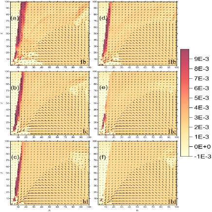
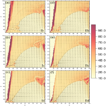
We now concentrate on how the outflow rate is affected by the Comptonization. Outflows move to very large distances and thus must not be bound to the system, i.e., the specific energy should be positive. Matter should also be of higher entropy as it is likely to be relativistic. Because of this we wish to concentrate on the behaviour of matter which have highest energy and entropy. Though we injected matter at the outer edge with a constant specific energy, the energy of matter in the post-shock region is redistributed due to turbulence, Compton cooling and shock heating. Some entropy is generated as well. The high energy and high entropy matter escape in the form of a hollow cone around the axis. It is thus expected that if the post-shock region itself is collapsed due to Comptonization, the outflows will also be quenched. We show this effect in our result. In Figure 8, we present the specific energy distribution for both the specific angular momenta (left panel for and right panel for ) for all the cooling Cases (marked in each box) at the end of our simulation. The velocity vectors are also plotted. The scale on the right gives the specific energy. First we note that the jets are stronger for higher angular momentum. This is because the post-shock region (between the shock and the inner sonic point close to the horizon) is hotter. Second, lesser and lesser amount of matter has higher energy as the cooling is increased. A similar observation could be made from Figure 9, where the entropy distribution is plotted. The jet matter having upward pointing vectors have higher entropy. However, this region shrinks with the increase in Keplerian rate, as the cooling becomes significant the outward thermal drive is lost. Here, the velocity vectors are of length at the outer boundary on the right and others are scaled accordingly.
In order to quantify the decrease in the outflow rates with cooling, we define two types of outflow rates. One is which is defined to be the rate at which outward pointing flow leaves the computational grid. This will include both the high and low energy components of the flow. In Figures 10(a) and (b), we show the results of time variation of the ratio ( / ) for the four cases (marked in each box), being the constant injection rate on the right boundary. While the ratio is clearly a time varying quantity, we observe that with the increase in cooling the ratio is dramatically reduced and indeed become almost saturated as soon as some cooling is introduced. Our rigorous finding once again verified what was long claimed to be the case, namely, the spectrally soft states (those having a relatively high Keplerian rate) have weaker jets because of the presence of weaker shocks [Chakrabarti, 1999, Das et al., 2001].
Another measure of the outflow rate would be to concentrate only those matter which have high positive energy and high entropy. For concreteness, we concentrate only on matter outflowing within at the upper boundary of our computational grid. We define this to be (). Figures 11(a) and 11(b) show time variation of . The different cases are marked on the curves. This outflow rate fluctuates with time. We easily find that the cooling process reduces this high energy component of matter drastically. Thus both the slow moving outflows and fast moving jets are affected by the Comptonization process at the base.
4.3 Spectral properties of the Disk-Jet system
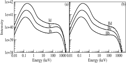
In each simulation we also store the photons emerging out of the Computational grid after exchanging energy and momentum with the free electrons in the disk matter. When the Keplerian disk rate is increased, the injected soft photons go up, cooling every electron in the sub-Keplerian halo component. Thus, the relative availability of the soft photons and the hot electrons in the disk and the jet dictates whether the emergent photons would be spectrally soft or hard. In Figures 12(a) and 12(b), we show three spectra for each of the specific angular momenta: (a) and (b) . The Cases are marked. We see that a spectrum is essentially made up of the soft bump (injected multi-colour black body spectrum from the Keplerian disk), and a Comptonized spectrum with an exponential cutoff – the cutoff energy being dictated by the electron cloud temperature. If we define the energy spectral index to be in the region keV, we note that increases, i.e., the spectrum softens with the increase in . This is consistent with the static model of Chakrabarti & Titarchuk [1995].
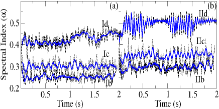
In reality, since the disk is not stationary, the spectrum also varies with time, and so is . In Figure 13, we present the time variation of the spectral index for the different Cases. We draw the running mean through these variations. We clearly see that the spectral index goes up with the increase in the disk accretion rate. Thus, on an average, the spectrum softens. We also find that the spectrum oscillates quasi-periodically and the frequency is higher for higher cooling rate. This agrees with the general observations that the QPO frequency rises with luminosity [Cui et al., 1999, Sobczak et al., 2000, McClintock et al., 2009].
It is interesting to understand the physical reason behind the shock oscillations. It has been argued by numerical simulation [Molteni et al., 1996, Chakrabarti et al., 2004] this oscillation is due to a resonance effect. When the cooling time scale roughly agrees with the infall time scale, the post-shock region, i.e., the CENBOL may oscillate. As the CENBOL oscillates, the high energy part of the spectrum also oscillates since the CENBOL is mainly responsible to energize the soft photons coming out from the Keplerian disk to high energy. Indeed, when we compute the cooling time scale and the infall time scale, we find that in all the cases when oscillations occur, the ratio of cooling time scale and infall time scale on an average remains within forty percent of each other. Of course, in the absence of cooling effects, some times the shock oscillations is possible when the Rankine-Hugoniot condition is not fulfilled [Ryu et al., 1997]. The amplitude of oscillation in this case is generally quite large and the result strongly depends on the specific angular momentum and specific energy of the flow. Observationally, different types of QPOs have been observed. This aspect requires a further study which is beyond the scope of this paper.
5 Concluding remarks
In this paper, we compute the effects of Compton cooling on the formation and rates of the outflows and jets. Most importantly, we study the variation of the spectral slope. We employ a hydrodynamic code based on the total variation diminishing method coupled to a Monte Carlo simulation to take care of the time dependent radiative transfer problem. We found many important results which can be briefly summarized as follows: (a) The increase in the Keplerian disk rate cools down the post-shock region of a sub-Keplerian flow and as a result the shock advances closer to the black hole. (b) The cooler and smaller sized post-shock region produced a weaker outflow/jet. (c) The spectrum becomes softer when the cooling is increased. (d) Quasi-periodic oscillations are produced as a result of near resonance between the cooing time scale as the infall time scale.
We coupled the hydrodynamics and Comptonization using a two step process. This is natural: Comptonization is strongly non-local process and the results are obtained by Monte Carlo method. However, the hydrodynamics code is a finite difference code. So at every instant both effects cannot be taken into account. The effects of radiative cooling or heating due to Comptonization is included in the hydrodynamics after each Monte Carlo step. After that the hydrodynamic code is advanced for a time period which is a factor of lower than the cooling or hydrodynamic time scale, whichever is lesser before running the Monte-Carlo step once more. Thus our dynamics is affected by the radiative cooling or heating effects.
In this context, it is important to note that the effects of radiation is not the same as in a single component flow. In a single component disk, such as the standard accretion disk, the radiation field is strong (especially when the accretion rate crosses the Eddington rate) as has been shown for example, by Ohsuga & Mineshige [2011]. However, in our case, the radiation field is important only if it interacted with electrons. In a two component flow, there are two effects which affect the dynamics of the electrons (a) the thermal acceleration depends on the gradient of thermal pressure and (b) the radiative acceleration depends on the number of Compton scattering and the amount of energy and momentum exchanged in the process (i.e., depends on local temperature). Both and have strong dependence on both the accretion rates. For a fixed halo rate, monotonically rises with disk rate but not exactly as in Ohsuga & Mineshige [2011], since the results depend on the optical depth of the halo. need not rise monotonically, however. We find that with the rise of the disk rate, initial rising trend of is reversed because the electrons are cooled down at a higher Keplerian disk rate, so the local temperature becomes low. We find that the ratio remains much less than unity even for .
Some of these results, as such, have been anticipated both theoretically and observationally. From the theoretical point of view [Chakrabarti & Titarchuk, 1995], in the two component model showed that the spectrum becomes softer. Similarly, Chakrabarti [1999] found that the outflow rate becomes smaller when shock becomes weaker. The shock oscillation model observations reported by Gallo et al. [2004], Fender et al. [2004] point to the same correlation between the spectral states and the outflow rates. However, it is the first time that we demonstrate the results with a complete coupled numerical simulations. The results we found are quite general and should be valid even for massive black holes, provided the cooling plays a role in the dynamics of the flow.
References
- Appl & Camenzind [1993] Appl, S., & Camenzind, M. 1993, A&A, 270, 71
- Blandford & Begelman [1999] Blandford, R. D., & Begelman, M. C. 1999, MNRAS, 303, L1
- Blandford & Payne [1982] Blandford, R. D., & Payne, D. G. 1982, MNRAS, 199, 883
- Blandford & Rees [1974] Blandford, R. D., & Rees, M. J. 1974, MNRAS, 169, 395
- Chakrabarti [1986] Chakrabarti, S. K. 1986, ApJ, 303, 582
- Chakrabarti [1998] Chakrabarti, S. K. 1998, arXiv:astro-ph/9801079
- Chakrabarti [1999] Chakrabarti, S. K. 1999, A&A, 351, 185
- Chakrabarti et al. [2004] Chakrabarti, S. K., Acharyya, K., & Molteni, D. 2004, A&A, 421, 1
- Chakrabarti & Titarchuk [1995] Chakrabarti, S. K., & Titarchuk, L.G. 1995, ApJ, 455, 623
- Chattopadhyay et al. [2004] Chattopadhyay, I., Das, S., & Chakrabarti, S. K. 2004, MNRAS, 348, 846
- Cui et al. [1999] Cui, W., Zhang, S. N., Chen, W., et al. 1999, ApJ, 512, L43
- Das & Chattopadhyay [2008] Das, S. & Chattopadhyay, I. 2008, New Astron., 13, 549
- Das et al. [2001] Das, S., Chattopadhyay, I., Nandi, A., & Chakrabarti, S. K. 2001, A&A, 379, 683
- Fender et al. [2004] Fender, R. P., Belloni, T. M., & Gallo, E. 2004, MNRAS, 355, 1105
- Fender et al. [2010] Fender, R. P., Gallo, E., & Russell, D. 2010, MNRAS, 406, 1425
- Fukue [1983] Fukue, J. 1983, PASJ, 35, 539
- Gallo et al. [2004] Gallo, E., Fender, R. P., & Pooley, G. 2004, NuPhS, 132, 363
- Ghosh et al. [2009] Ghosh, H., Chakrabarti, S. K., & Laurent, P. 2009, IJMPD, 18, 1693
- Ghosh et al. [2010] Ghosh, H., Garain, S. K., Chakrabarti, S. K., & Laurent, P. 2010, IJMPD, 19, 607
- Ghosh et al. [2011] Ghosh, H., Garain, S. K., Giri, K., & Chakrabarti, S. K. 2011, MNRAS, 416, 959
- Giri et al. [2010] Giri, K., Chakrabarti, S. K., Samanta, M. M., & Ryu, D. 2010, MNRAS, 403, 516
- Giri & Chakrabarti [2012] Giri, K., & Chakrabarti, S. K. 2012, MNRAS, 421, 666
- Hawley & Balbus [1992] Hawley, J. F., & Balbus, S. A. 1992, ApJ, 400, 595
- Hawley et al. [1984] Hawley, J. F., Smarr, L. L., & Wilson, J. R. 1984, ApJS, 55, 211
- Igumenshchev et al. [1998] Igumenshchev, I. V., Abramowicz, M. A., & Novikov, I. D. 1998, MNRAS, 298, 1069
- Igumenshchev et al. [1996] Igumenshchev, I. V., Chen, X., & Abramowicz, M. A. 1996, MNRAS, 278, 236
- Junor et al. [1999] Junor, W., Biretta, J. A. & Livio, M. 1999, Nature, 401, 891
- Lanzafame et al. [1998] Lanzafame, G., Molteni, D., & Chakrabarti, S. K. 1998, MNRAS 299 799
- McClintock et al. [2009] McClintock, J. E., Remillard, R. A., Rupen, M. P., et al. 2009, ApJ, 698, 1398
- Molteni et al. [1994] Molteni, D., Lanzafame, G., & Chakrabarti, S. K. 1994, ApJ, 425, 161
- Molteni et al. [1996] Molteni, D., Ryu, D., & Chakrabarti, S. K. 1996, ApJ, 470, 460
- Molteni et al. [1996] Molteni, D., Sponholz, H., & Chakrabarti, S. K. 1996, ApJ, 457, 805
- Narayan & Yi [1995] Narayan, R. & Yi, I. 1995, ApJ, 452, 710
- Niedzwiecki et al. [1997] Niedzwiecki, A. M., Krolik, J. H., & Zdziarski, A. 1997, ApJ, 483, 111
- Ohsuga & Mineshige [2011] Ohsuga, K., & Mineshige, S. 2011, ApJ, 736, 2
- Paczyński & Wiita [1980] Paczyński, B., & Wiita, P. J. 1980, A&A, 88, 23
- Pozdnyakov et al. [1983] Pozdnyakov, A., Sobol, I. M., & Sunyaev, R. A. 1983, Astrophys. Space Sci. Rev., 2, 189
- Rybicki & Lightman [1979] Rybicki, G. B., & Lightman, A. P. 1979, Radiative Processes in Astrophysics (John Wiley & Sons, New York)
- Ryu et al. [1995] Ryu, D., Brown, G. L., Ostriker, J. P., & Loeb, A. 1995, ApJ, 452, 364
- Ryu et al. [1997] Ryu, D., Chakrabarti, S. K., & Molteni, D. 1997, ApJ, 474, 378
- Shakura & Sunyaev [1973] Shakura, N. I., & Sunyaev, R. A. 1973, A&A, 24, 337
- Singh & Chakrabarti [2011] Singh, C. B., & Chakrabarti, S. K. 2011, MNRAS, 410, 2414
- Smith et al. [2001] Smith, D. M., Heindl, W. A., Markwardt, C. B., & Swank, J. H. 2001, ApJ, 554, L41
- Smith et al. [2002] Smith, D. M., Heindl, W. A., & Swank, J. H. 2002, ApJ, 569, 362
- Sobczak et al. [2000] Sobczak, G. J., Mcclintock, J. E., Remillard, R. A., et al. 2000, ApJ, 531, 537
- Soria et al. [2001] Soria, R., Wu, K., Hannikainen, D., McMollough, M. & Hunstead, R. 2001, Proceedings of a joint workshop held by the Center for Astrophysics (Johns Hopkins University) and the Laboratory for High Energy Astrophysics (NASA/ Goddard Space Flight Center) in Baltimore, MD; Eds.: T. Yaqoob and J. H. Krolik
- Wu et al. [2002] Wu, K., Soria, R., & Campbell-Wilson, D., et al. 2002, ApJ, 565, 1161