The first planet detected in the WTS: an inflated hot-Jupiter in a 3.35 day orbit around a late F-star

Abstract

We report the discovery of WTS-1b, the first extrasolar planet found by the WFCAM Transit Survey, which began observations at the 3.8-m United Kingdom Infrared Telescope. Light curves comprising almost 1200 epochs with a photometric precision of better than 1 per cent to $J\sim 16$ were constructed for $\sim 60\,000$ stars and searched for periodic transit signals. For one of the most promising transiting candidates, high-resolution spectra taken at the Hobby-Eberly Telescope allowed us to estimate the spectroscopic parameters of the host star, a late-F main sequence dwarf (V=16.13) with possibly slightly subsolar metallicity, and to measure its radial velocity variations. The combined analysis of the light curves and spectroscopic data resulted in an orbital period of the substellar companion of 3.35 days, a planetary mass of 4.01$\pm$0.35 $M_{J}$, and a planetary radius of $1.49^{+0.16}_{-0.18}$ $R_{J}$. WTS-1b has one of the largest radius anomalies among the known hot Jupiters in the mass range 3-5 $M_{J}$.

1 Introduction

The existence of highly-irradiated, gas-giants planets orbiting within $<0.1$ AU of their host stars, and the unexpected large radii of many of them, is an unresolved problem in the theory of planet formation and evolution (Baraffe et al., 2010). Their prominence amongst the $777$ confirmed exoplanets is unsurprising; their large radii, large masses, and short orbital periods make them readily accessible to ground-based transit and radial velocity surveys, on account of the comparatively large flux variations and reflex motions that they cause. Exoplanet searches often focus on the detection of small Earth-like exoplanets, but understanding the formation mechanism and evolution of the giant planets, particularly in the overlap mass regime with brown dwarfs, is a key question in astrophysics.

This paper reports on WTS-1b, the first planet discovery from the WFCAM Transit Survey (WTS; Kovács et al. 2012; Birkby et al. 2011). The WTS is the only large-scale ground-based transit survey that operates at near infrared (NIR) wavelengths. The advantage of photometric monitoring at NIR wavelengths is an increased sensitivity to photons from M-dwarfs ($M_{\star}<0.6$ $M_{\odot}$). These small stars undergo similar flux variations and reflex motions in the presence of an Earth-like companion as solar-type stars do with hot Jupiter companions. While a primary goal of the WTS is the detection of terrestrial planets around cool stars, WTS can also provide observational constraints on the mechanism for giant planet formation, by accurately measuring the hot Jupiter fraction for M-dwarfs. The light curve quality of the WTS is sufficient to reveal transiting super-Earths around mid-M dwarfs (Kovács et al., 2012), but scaling-up means that any hot Jupiter companions to the $\sim$80 000 FGK stars in the survey are also detectable.

Theoretical models of isolated giant planets predict an almost constant radius for pure H$+$He objects in the mass range $0.5-10$ $M_{J}$ as a result of the equilibrium between the electron degeneracy in the core and the pressure support in the external gas layers (Zapolsky & Salpeter, 1969; Guillot, 2005; Seager et al., 2007; Baraffe et al., 2010). Hence the larger radii of many hot Jupiters (hereafter HJ) must arise from other factors. Due to the proximity of these planets to their host star, the irradiation of the surface of the planet is thought to play a major role in the so-called radius anomaly, by altering the thermal equilibrium and delaying the Kelvin-Helmholtz contraction of the planet from birth (e.g. Showman & Guillot, 2002). This is supported by a correlation between the mean planetary density and the incident stellar flux (Laughlin et al., 2010; Demory & Seager, 2011; Enoch et al., 2012). However, it has been shown that this cannot be the only explanation for the radius anomaly (Burrows et al., 2007), and other sources must contribute to the large amount of energy required to keep gas giants radii above $\sim$1.2 $R_{J}$ (Baraffe et al., 2010).

There are a number of physical mechanisms thought to be responsible for radius inflation, including (but not limited to): tidal heating due to the circularisation of close-in orbits (Bodenheimer et al., 2001, 2003; Jackson et al., 2008), reduced heat loss due to enhanced opacities in the outer layers of the planetary atmosphere (Burrows et al., 2007), double-diffusive convection leading to slower heat transportation (Chabrier et al., 2007; Leconte & Chabrier, 2012), increased heating via Ohmic dissipation in which ionised atoms interact with the planetary magnetic field as they move along strong atmospheric winds (Batygin & Stevenson, 2010), and a slower cooling rate due to the mechanical greenhouse effect in which turbulent mixing drives a downwards flux of heat simulating a more intense incident irradiation (Youdin & Mitchell, 2010). A radically different explanation has been proposed by Martín et al. (2011) who point out a correlation between radius anomaly and tidal decay timescale and suggest that inflated HJs are actually young because they have recently formed as a result of binary mergers. Studying the radius anomaly in higher mass HJs ($>3$ $R_{J}$) is useful as they are perhaps more resilient to atmospheric loss due to their larger Roche lobe radius.

This paper is organised as follows: in Section 1.1 we briefly describe the strategy of the WFCAM Transit Survey, while the photometric and spectroscopic observations are presented in Section 2.1 along with their related data reduction. Section 3 describes how we characterized the host star (Section 3.1) and determined the properties of the planet (Section 3.2), using a combination of low- and high-resolution spectra and photometric follow-up observations. A discussion on the nature and the peculiarity of this new planet, our conclusions and further considerations are given in Section 4. Throughout this paper we refer to the planet as WTS-1b, and to the parent star and the whole star-planet system as WTS-1.

1.1 The WFCAM Transit Survey

The WTS is an on-going photometric monitoring campaign using the Wide Field Camera (WFCAM) on the United Kingdom Infrared Telescope (UKIRT) at Mauna Kea, Hawaii, and has been in operation since August 2007. UKIRT is a 3.8-m telescope, designed solely for NIR observations and operated in queue-scheduled mode. The survey was awarded 200 nights of observing time, of which $\sim$50$\%$ has been observed to-date, and runs primarily as a back-up program when observing conditions are not optimal for the main UKIDSS programs (seeing $>1$ arcsec). The survey targets four 1.6 deg² fields, distributed seasonally in right ascension at 03, 07, 17 and 19 hours to allow year-round visibility. WTS-1b is located in the 19 hour field (hereafter 19hr). The fields are close to the Galactic plane but have $b>5$ degrees to avoid over-crowding and high reddening. The exact locations were chosen to maximise the number of M-dwarfs, while keeping giant contamination at a minimum and maintaining an $E(B-V)<0.1$. Due to the back-up nature of the program, observations of a given field are randomly distributed throughout a given night, but on average occur in a one hour block at its beginning or end. Seasonal visibility also leaves long gaps when no observations are possible (Kovács et al., 2012). Since the WTS was primarily designed to find planets transiting M-dwarf stars, the observations are obtained in the J-band ($\sim$1.25 $\mu$m). This wavelength is near to the peak of the spectral energy distribution (SED) of a typical M-dwarf. Hotter stars, with an emission peaking at shorter wavelength, are consequently fainter in this band. Interestingly, photometric monitoring at NIR wavelengths may have a further advantage as it is potentially less susceptible to the effect of star-spot induced variability (Goulding et al., 2012). The discovery reported in this paper demonstrates that despite the survey optimisation for M-dwarfs, its uneven epoch distribution and the increased difficulty in obtaining high-precision light curves from ground-based infrared detectors, it is still able to detect HJs around FGK stars.

2 Observations

2.1 Photometric data

2.1.1 UKIRT/WFCAM $J$-band photometry

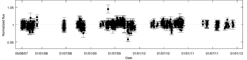
Figure 1: The unfolded $J$-band light curve for WTS-1.

Table 1: WFCAM $J$-band light curve. The full epoch list, which contains 1 182 entries, will be available electronically.

HJD	Normalized	Error
-2 400 000	flux
54317.8138166	1.0034	0.0057
54317.8258565	0.9971	0.0056
…	…	…
55896.7105702	0.9979	0.0064

The instrument used for this campaign is WFCAM (Casali et al., 2007), which has a mosaic of four Rockwell Hawaii-II PACE infrared imaging 2048 $\times$ 2048 pixels detectors, covering $13.65\arcmin\times 13.65\arcmin$ ($0.4\arcsec$/pixel) each. The detectors are placed in the four corners of a square (this pattern is called a paw-print) with a separation of $12.83\arcmin$ between the chips, corresponding to $94\%$ of a chip width. Each of the four fields consists of eight pointings of the WFCAM paw-print, each one comprising a 9-point jitter pattern of 10 second exposures each, and tiled to give uniform coverage across the field. It takes 15 minutes to observe an entire WTS field ($9\times 10s\times 8$ + overheads). In this way, the NIR light-curves have an average cadence of 4 data points per hour.

A full description of our 2-D image processing and light curve generation is given by Kovács et al. (2012) and closely follows that of Irwin et al. (2007). Briefly, a modified version of the CASU INT wide-field survey pipeline (Irwin & Lewis, 2001) is used to remove the dark current and reset anomaly from the raw images, apply a flat-field correction using twilight flats, and to decurtain and sky subtract the final images. Astrometric and photometric calibration is performed using 2MASS stars in the field-of-view (Hodgkin et al., 2009). A master catalogue of source positions is generated from a stacked image of the 20 best frames and co-located, variable aperture photometry is used to extract the light curves. We attempt to remove systematic trends that may arise from flat-fielding inaccuracies or varying differential atmospheric extinction across the image by fitting a 2-D quadratic polynomial to the flux residuals in each light curve as a function of the source’s spatial position on the chip. As a final correction, for each source we remove residual seeing-correlated effects by fitting a second-order polynomial to the correlation between its flux and the stellar image FWHM per frame (see Irwin et al. 2007 for a discussion of the effectiveness of these techniques).

The final $J$-band light curves have a photometric precision of 1$\%$ down to $J=16$ mag ($\sim$7$\%$ for $J=18$ mag while the uncertainty per data point is just 3 mmag for the brightest stars (saturation occurs between $J\sim 12-13$ mag). The unfolded $J$-band light curve for WTS-1 is shown in Figure 1 (all the measurements are reported in Table 1) and its final out-of-transit RMS is 0.0064 (equivalent to 6.92 mmag).

2.1.2 Transit detection algorithm

Table 2: The host star WTS-1.

[b] Parameter Value RA^a 19h 35m 58.37s Dec^a +36d 17m 25.17s l^a +70.0140 deg b^a +7.5486 deg $\mu_{\alpha}cos\delta$^b -7.7$\pm$2.4 mas yr^-1 $\mu_{\delta}$^b -2.8$\pm$2.4 mas yr^-1

• Epoch J2000;

• Proper motion from SDSS.

We identified WTS-1b in the $J$-band light curves by using the Box-Least-Squares transit search algorithm occfit, as described in Aigrain & Irwin (2004), which takes a maximum likelihood approach to fitting generalized periodic step functions. Before inspecting transit candidates by eye, we employed several criteria to speed up the detection process. The first is a magnitude cut, in which we removed all sources fainter than $J=17$ mag. We also required that the source have an image morphology consistent with stellar sources (Irwin et al., 2007). Despite our attempts to remove systematic trends in the light curves, we invariably suffered from residual correlated red noise, so we modified the detection significance statistic, $S$, from occfit according to the prescription (equation 4) of Pont et al. (2006), to obtain $S_{red}$. Our transit candidates must then have $S_{red}\geq 5$ to survive, although we note that this is more permissive with respect to the limit recommended by Pont and collaborators ($S_{red}\geq 7$). We further discarded any detections with a period in the range $0.99<$P$<1.005$ days, in order to avoid the common $\sim$1 day alias of the ground-based photometric surveys.

Next, as fully described in Birkby et al. (2012a), the WFCAM $ZYJHK$ single epoch photometry was combined with five more optical photometric data points ($ugriz$ bands) available for the 19hr field from the Sloan Digitized Sky Survey archive (SDSS $7^{th}$ release, Nash, 1996) to create an initial SED. The SEDs were fitted with the NextGen models (Baraffe et al., 1998) in order to estimate effective temperatures and hence a stellar radius for each source. We could then impose a final threshold on the detected transit depths, by rejecting those that corresponded to a planetary radius greater than 2 $R_{J}$. It is worth noting that occfit tends to under-estimate transit depths because it does not consider limb-darkening effects and the trapezoidal shape of the transits. Moreover, the NextGen models systematically under-estimate the temperature of solar-like stars (Baraffe et al., 1998), so the initial radius estimates are also under-predicted. Hence, the genuine HJ transit events are unlikely to be removed in this final threshold cut. As a result, our transits detection procedure was conservative. Many of the $\sim$3 500 phase-folded light curves which satisfied our criteria were false-positives arising from nights of bad data or single bad frames. Others were binary systems, folded on half the true orbital period. A more detailed analysis of the candidate selection procedure and of advanced selection steps in the survey can be found in Sipőcz et al. (2012).

The WTS-1 $J$-band light curve passed all our selection criteria and the object (see Table 2) progressed to the following phases of candidate’s confirmation. The descriptions of the photometric and spectroscopic data in the next sections are organized in order to match the following chronological sequence of analysis. First, optical $i^{\prime}$-band photometric follow-up of WTS-1 was conduced in order to prove the real presence of the transit and check the transit depth consistency between the two bands. Then, ISIS/WHT intermediate resolution spectra enabled us to place strong constrains on the velocity amplitude of host star (at the km s^-1level) and therefore to rule out the false-positive eclipsing binaries scenarios. Finally we moved to the high-resolution spectroscopic follow-up. The confirmation of the planetary nature of WTS-1b came with the RV measurements obtained with the HET spectra.

2.1.3 Broad band photometry

The WFCAM and SDSS photometric data for WTS-1 are reported in Table 3 with other single epoch broad band photometric observations. Johnson $B$ $V$ $R$ bands were observed for WTS-1 on the night of 6th April 2012 at the University of Hertfordshire’s Bayfordbury Observatory. We used a Meade LX200GPS 16-inch f/10 telescope fitted with an SBIG STL-6303E CCD camera, and integration times of 300 seconds per band. Images were bias, dark, and flat-field corrected, and extracted aperture photometry was calibrated using three bright reference stars within the image. Photometric uncertainties combine contributions from the SNR of the source (typically $\sim$20) with the scatter in the zero point from the calibration stars. The Two Micron All Sky Survey (2MASS, Skrutskie et al., 2006) and the Wide-field Infrared Survey Explorer (WISE, Wright et al., 2010) provide further NIR data points ($J$ $H$ $Ks$ bands and $W1$ $W2$ bands respectively).

Table 3: Broad band photometric data of WTS-1 measured within the WFCAM (Vega), SDSS (AB), 2MASS (Vega) and WISE (Vega) surveys. Johnson magnitudes in the visible are provided too (Vega). Effective wavelength $\lambda_{eff}$ (mean wavelength weighted by the transmission function of the filter), equivalent width (EW) and magnitude are given for each single pass-band. The bands are sorted by increasing $\lambda_{eff}$.

Band	$\lambda_{eff}$[Å]	EW[Å]	Magnitude
SDSS-u	3546	558	18.007 ($\pm$0.014)
Johnson-B	4378	970	17.0 ($\pm$0.1)
SDSS-g	4670	1158	16.785 ($\pm$0.004)
Johnson-V	5466	890	16.5 ($\pm$0.1)
SDSS-r	6156	1111	16.434 ($\pm$0.004)
Johnson-R	6696	2070	16.1 ($\pm$0.1)
SDSS-i	7471	1045	16.249 ($\pm$0.004)
UKIDSS-Z	8817	879	15.742 ($\pm$0.005)
SDSS-z	8918	1124	16.189 ($\pm$0.008)
UKIDSS-Y	10305	1007	15.642 ($\pm$0.007)
2MASS-J	12350	1624	15.375 ($\pm$0.052)
UKIDSS-J	12483	1474	15.387 ($\pm$0.005)
UKIDSS-H	16313	2779	15.103 ($\pm$0.006)
2MASS-H	16620	2509	15.187 ($\pm$0.081)
2MASS-Ks	21590	2619	15.271 ($\pm$0.199)
UKIDSS-K	22010	3267	15.048 ($\pm$0.009)
WISE-W1	34002	6626	15.041 ($\pm$0.044)
WISE-W2	46520	10422	15.886 ($\pm$0.157)

2.1.4 INT $i^{\prime}$-band data

In addition to the WFCAM $J$-band light curve, we observed one half transit of the WTS-1 system in the $i^{\prime}$-band using the Wide Field Camera on the 2.5-m Isaac Newton Telescope (McMahon et al., 2001) on July 23, 2010. A total of 82 images, sampling the ingress of the transit, were taken with an integration time of 60 seconds. The data were reduced with the CASU INT/WFC data reduction pipeline as described in detail by Irwin & Lewis (2001) and Irwin et al. (2007). The pipeline performs a standard CCD reduction, including bias correction, trimming of the overscan and non-illuminated regions, a non-linearity correction, flat-fielding and defringing, followed by astrometric and photometric calibration. A master catalogue for the $i^{\prime}$-band filter was then generated by stacking 20 frames taken under the best conditions (seeing, sky brightness and transparency) and running source detection software on the stacked image. The extracted source positions were used to perform variable aperture photometry on all of the images, resulting in a time-series of differential photometry.

The final out-of-transit RMS in the WTS-1 $i^{\prime}$-band light curve is 0.0026 (equivalent to 2.87 mmag) and is used to refine the transit model fitting procedure in Section 3.2.1. The $i^{\prime}$-band light curve for WTS-1 is given in Table 4.

Table 4: INT $i^{\prime}$-band light curve of WTS-1. The full epoch list, which contains 82 entries, will be available electronically.

HJD	Normalized	Error
-2 400 000	flux
55401.3703254	1.0244	0.0109
55401.3809041	1.0205	0.0034
…	…	…
55401.4894461	0.9936	0.0022

2.2 Spectroscopic data

2.2.1 ISIS/WHT

We carried out intermediate-resolution spectroscopy of the star WTS-1 over two nights between July $29-30$, 2010, as part of a wider follow-up campaign of the WTS planet candidates, using the William Herschel Telescope (WHT) at Roque de Los Muchachos, La Palma. We used the single-slit Intermediate dispersion Spectrograph and Imaging System (ISIS). The red arm with the R1200R grating centred on 8500 Å was employed. We did not use the dichroic during the ISIS observations because it can induce systematics and up to $10\%$ efficiency losses in the red arm, which we wanted to avoid given the relative faintness of our targets. The four spectra observed have a wavelength coverage of 8100–8900 Å. The wavelength range was chosen to be optimal for the majority of the targets for our spectroscopic observation which were low-mass stars. The slit width was chosen to match the approximate seeing at the time of observation giving an average spectral resolution $R\sim 9000$. An additional low-resolution spectrum was taken on July 16th, 2010, using the ISIS spectrograph with the R158R grating centred on 6500 Å. This spectrum has a resolution ($R\sim 1000$), a SNR of $\sim 40$ and a wider wavelength coverage (5000–9000 Å). The spectra were processed using the iraf.ccdproc package for instrumental signature removal. We optimally extracted the spectra and performed wavelength calibration using the semi-automatic kpno.doslit package. The dispersion function employed in the wavelength calibration was performed using CuNe arc lamp spectra taken after each set of exposures.

2.2.2 CAFOS/2.2-m Calar Alto

Two spectra of WTS-1 were obtained with CAFOS at the 2.2-m telescope at the Calar Alto observatory (as a Director’s Discretionary Time - DDT) in June, 2011. CAFOS is a 2k${\times}$2k CCD SITe#1d camera at the RC focus, and it was equipped with the grism R-100 that gives a dispersion of ${\sim}$ 2.0 Å/pix and a wavelength coverage from 5850 to 9500 Å, approximately. Their resolving power is of around $R\sim 1900$ at 7500 Å, with a $SNR\sim 25$. The data reduction was performed following a standard procedure for CCD processing and spectra extraction with iraf. The spectra were finally averaged in order to increase the SNR.

2.2.3 KPNO

A low resolution spectrum of WTS-1 was observed in September 2011 with the Ritchey-Chretien Focus Spectrograph at the 4-m telescope at Kitt Peak (Arizona, USA). The grism BL-181, which gives a dispersion of ${\sim}$ 2.8 Å/pix, was used. Calibration, sky subtraction, wavelength and flux calibration were performed following a standard procedure for long slit observations using dedicated iraf tasks. The ThAr arc lamp and the standard star spectra, employed for the wavelength and the flux calibration respectively, were taken directly after the science exposure. The measured spectrum covers the wavelength range 6000-9000 Å with SNR$\sim$40 at 7500 Å and has a resolution of $R\sim 1000$. This is the only flux calibrated spectrum we have available.

2.2.4 HET

In the late 2010 and in the second half of the 2011 the star WTS-1 was observed during 11 nights with the High Resolution Spectrograph (HRS) housed in the insulated chamber in the basement of the 9.2-m segmented mirror Hobby-Eberly Telescope (HET, see Ramsey et al., 1998). The HRS is a single channel adaptation of the ESO UVES spectrometer linked to the corrected prime focus of the HET through its fiber-fed instrument as described by Tull (1998). It uses an R-4 echelle mosaic, which we used with a resolution of R=60 000, and a cross-dispersion grating to separate spectral orders, while the detector is a mosaic of two thinned and anti-reflection coated 2K $\times$ 4K CCDs.

One science fiber was used to get the spectrum of the target star and two sky fibers were used in order to subtract the sky contamination. A couple of ThAr calibration exposures were taken immediately before and after the science exposure. This strategy allowed us to keep under control any undesired systematic effect during the observation. Each science observation (except one, see Section 3.2.2) was split in two exposures, of about half an hour each, in order to limit the effect of the cosmic rays hits, which can affect the data reduction and analysis steps. Due to the faintness of the star, the Iodine gas cell was not used for our observations.

The data reduction was performed with the iraf.echelle package (Willmarth & Barnes, 1994). After the standard calibration of the raw science frame, bias-subtraction and flat-fielding, the stellar spectra were extracted order by order and the related sky spectrum was subtracted. The extracted ThAr spectra were used to compute the dispersion functions, which are characterized by an RMS of the order of 0.003 Å. Consistency between the two solutions (computed from the ThAr taken before and after the science exposure) was checked for all the nights in order to detect possible drifts or any other technical hitch that could take place during each run. Successively, the spectra were wavelength calibrated using a linear interpolation of the two dispersion functions.

In the subsequent data analysis, custom Matlab programs were used. After the continuum estimation and the following normalization, the spectra were filtered to remove the residual cosmic rays peaks left after the previous filtering performed on the raw science frame with the iraf task cosmicrays. Comparing the spectra of all the nights for each single order, the pixels with higher flux, due to a cosmic hit on the detector, were detected and masked. The telluric absorption lines present in the redder orders were then removed in order to avoid contaminations using a high SNR observed spectrum of a white dwarf as template for the telluric lines. Finally, the spectra related to the two split science exposures were averaged to obtain the final set of spectra used in the following analysis. A total of 40 orders (18 from the red CCD and 22 from the blue one) cover the wavelength range 4400-6300 Å. The spectra have a SNR $\sim 8$.

3 Analysis and results

3.1 Stellar parameters

3.1.1 Spectral energy distribution

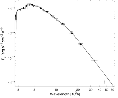
Figure 2: Broad band photometric data of WTS-1: SDSS (filled dots), Johnson (empty dots), WFCAM (squares), 2MASS (triangles) and WISE (stars). The best fitting template (black line) is the ATLAS9 Kurucz $T_{\rm{eff}}$=6500 K, log $g$=4.5, $[\rm{Fe/H}]$=-0.5 model with $A_{V}$=0.44. Vertical errorbars correspond to the flux uncertainties while those along the X-axis represent each band’s EW (see Table 3).

A first characterization of the parent star can be performed comparing the shape of the Spectral Energy Distribution (SED), constructed from broad band photometric observations, with a grid of synthetic theoretical spectra. The data relative to the photometric bands, collected in Table 3, were analysed with the application VOSA (Virtual Observatory SED Analyser, Bayo et al., 2008, 2012). VOSA offers a valuable set of tools for the SED analysis, allowing the estimation of the stellar parameters. It can be accessed through its web-page interface and accepts as input file an ASCII table with the following data: source identifier, coordinates of the source, distance to the source in parsecs, visual extinction ($A_{V}$), filter label, observed flux or magnitude and the related uncertainty. For our purpose, we tried to estimate only the main intrinsic parameters of the star: effective temperature, surface gravity and metallicity. The extinction $A_{V}$ was assumed as a further free parameter.

The synthetic photometry is calculated by convolving the response curve of the used filter set with the theoretical synthetic spectra. Then a statistical test is performed, via $\chi^{2}_{\nu}$ minimization, to estimate which set of synthetic photometry best reproduces the observed data. We decided to employ the Kurucz ATLAS9 templates set (Castelli et al., 1997) to fit our photometric data. These templates reproduce the SEDs in the high temperature regime better than the NextGen models (Baraffe et al., 1998), more suitable at lower temperatures ($<4500\,K$).

In order to speed up the fitting procedure, we restricted the range of $T_{\rm{eff}}$ and log $g$ to 3500-8000 K and 3.0-5.0, respectively. These constrains in the parameter space did not affect the final results as it was checked a posteriori that the same results were obtained considering the full available range for both parameters. The resulting best fitting synthetic template, plotted in Figure 2 with the photometric data, corresponds to the $T_{\rm{eff}}$=6500 K, log $g$=4.5 and $[\rm{Fe/H}]$=-0.5 Kurucz model and A_V=0.44. Uncertainties on the parameters were estimated both using $\chi^{2}_{\nu}$ statistical analysis and a bayesian (flat prior) approach. The related errors result to be of the order of 250 K, 0.2, 0.5 and 0.07 for $T_{\rm{eff}}$, log $g$, $[\rm{Fe/H}]$ and A_V, respectively.

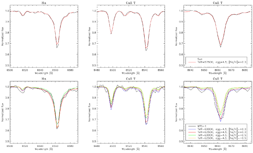
Figure 3: $Upper$ $row$: comparison of a degraded spectrum of the Sun (black) with a synthetic spectrum (red) computed with $T_{\rm{eff}}$=5750 K, log $g$=4.5 and $[\rm{Fe/H}]$=0.0. $Lower$ $row$: comparison of the WTS-1 spectrum (black) with different synthetic spectra (colours). The comparison between the observed WTS-1 spectrum and the synthetic models took into account the differences of the core of the lines shown in the upper row plots. From this analysis, the best fitting model is the one with $T_{\rm{eff}}$=6250 K, log $g$=4.5 and $[\rm{Fe/H}]$=0.0.

As it can be seen in Figure 2, the WISE $W2$ data point is not consistent with the best fitting model. Firstly, it is worth noting that the observed value of $W2=15.886$ ($\pm$0.157) is below the 5 sigma point source sensitivity expected in the $W2$-band ($>15.5$). The number of single source detections used for the $W2$-band measurement is also considerably less than that of the $W1$-band (4 and 19 respectively) increasing the uncertainty in the measurement. Finally, the poor angular resolution of WISE in the $W2$-band ($6.4\arcsec$) could add further imprecisions to the final measured flux, especially in a field as crowded as the WTS 19hrs field. For these reasons, the WISE $W2$ data point was not considered in the fitting procedure.

Once the magnitude values were corrected for the interstellar absorption according to the best fitting value (A_V=0.44$\pm$0.07), colour – temperature relations were used to further check the effective temperature and spectral type of the host star. From the SDSS $g$ and $r$ magnitudes, we obtained a value of (B-V)₀=0.43$\pm$0.04 (Jester et al., 2005) which imply $T_{\rm{eff}}$=6300$\pm$600 K assuming log $g$=4.4 and $[\rm{Fe/H}]$=-0.5 (Sekiguchi & Fukugita, 2000). Following the appendix B of Collier Cameron et al. (2007), the 2MASS ($J-H$) index of 0.23$\pm$0.09 leads to a value of $T_{\rm{eff}}$=6200$\pm$400 K while Table 3 of Covey et al. (2007) suggests the host star to be a late-F considering different colour indices at once. These results are all compatible within the uncertainties.

3.1.2 Spectroscopic analysis

The spectroscopic spectral type determination was done firstly by comparing the spectrum observed with CAFOS with a set of spectra of template stars. Stars of different spectral types, uniformly spanning the F5 to G2 range, were observed with the same instrumental setting. Since the observed spectrum has a relatively low SNR, we focused the analysis on the strongest features present which are the H$\alpha$ (6562.8 Å) and the Ca ii triplet (8498.02 Å, 8542.09 Å, 8662.14 Å). The best match was obtained, via minimization of the RMS of the difference between the WTS-1 and template star spectra, with the spectrum of an F6V star with solar metallicity.

Afterwards, we tried to estimate the stellar parameters comparing the observed spectrum with a simulated spectrum with known parameters. For that aim, we used a library of high resolution synthetic stellar spectra by Coelho et al. (2005), created by the PFANT code (Barbuy, 1982; Cayrel et al., 1991; Barbuy et al., 2003) that computes a synthetic spectrum assuming local thermodynamic equilibrium (LTE). The synthetic spectra were achieved using the model atmospheres presented by Castelli & Kurucz (2003). Since the core of these lines are strongly affected by cumulative effects of the chromosphere, non-LTE (local thermodynamical equilibrium) and inhomogeneity of velocity fields, we firstly compared a spectrum of the Sun observed with HIRES spectrograph at the Keck telescope (Vogt et al., 1994). The spectrum of the Sun was degraded to lower resolution and resampled to match our CAFOS spectrum specifications to see how such effects appear at this resolution and how different the solar spectrum is from a synthetic spectrum from the library by Coelho and collaborators. Looking at the upper plots in Figure 3, we concluded that the cores of the lines in the simulated spectrum are systematically higher than those in the observed spectrum of the Sun. Nevertheless, the Ca ii triplet line at 8498.02 Å seems to be less affected by the above-mentioned problems. Considering these differences between central depth of the observed and simulated spectra in the best fitting procedure, we estimated that the synthetic model with $T_{\rm{eff}}$=6250 K, log $g$=4.5 and $[\rm{Fe/H}]$=0.0 best reproduces the observed spectrum of WTS-1. The expected uncertainties are of the order of the step size of the used library ($\delta$$T_{\rm{eff}}$=250 K, $\delta$log $g$=0.5 and $\delta$$[\rm{Fe/H}]$=0.5).

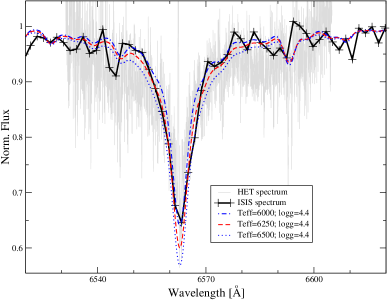
Figure 4: Intermediate resolution ISIS spectrum (black line) and high resolution HET spectrum (grey line) of the H$\alpha$ line of WTS-1 in comparison with synthetic spectra calculated with different effective temperatures of 6000 K (blue dash-dotted line), 6250 K (dashed line; finally adopted $T_{\rm{eff}}$), and 6500 K (blue dotted line). The synthetic spectra were convolved in order to match the resolution of the ISIS spectrum.

The high resolution HET spectra were employed to attempt a more detailed spectroscopic analysis of the host star. The spectra observed each single night were stacked together obtaining a final spectrum with a SNR of about 12, calculated over a 1 Å region at 5000 Å. To compute model atmospheres, LLmodels stellar model atmosphere code (Shulyak et al., 2004) was used. For all the calculations, LTE and plane-parallel geometry were assumed. We used the VALD database (Piskunov et al., 1995; Kupka et al., 1999; Ryabchikova et al., 1999) as a source of atomic line parameters for opacity calculations with the LLmodels code. Finally, convection was implemented according to the Canuto & Mazzitelli (1991) model of convection.

The parameter determination and abundance analysis were performed iteratively, self-consistently recalculating a new model atmosphere any time one of the parameters, including the abundances, changed. As a starting point, we adopted the parameters derived from the CAFOS spectrum. We performed the atmospheric parameter determination by imposing the iron excitation and ionization equilibria making use of equivalent widths measured for all available unblended and weakly blended lines. We converted the equivalent width of each line into an abundance value with a modified version (Tsymbal, 1996) of the WIDTH9 code (Kurucz, 1993). Unfortunately, the faintness of the observed star, coupled with the calibration process (including the sky subtraction), led to a distortion of the stronger lines, weakening their cores. For this reason, our analysis took into account only the measurable weak lines, making therefore impossible a determination of the microturbulence velocity ($v_{mic}$), which we fixed at a value of 0.85 km s^-1 (Valenti & Fisher, 2005). With the fixed $v_{mic}$, we imposed the Fe excitation and ionization equilibria, which led us to an effective temperature of 6000$\pm$400 K and a surface gravity of 4.3$\pm$0.4. Imposing the ionization equilibrium we took into account the expected non-LTE effects for Fe i ($\sim$0.05 dex, Mashonkina, 2011), while for Fe ii non-LTE effects are negligible.

In this temperature regime, the ionization equilibrium is sensitive to both $T_{\rm{eff}}$ and log $g$ variations, therefore it is important to simultaneously and independently further constrain temperature and/or gravity. For this reason we looked at the H$\alpha$ line to further constrain $T_{\rm{eff}}$, as in this temperature regime H$\alpha$ is sensitive primarily to temperature variations (Fuhrmann et al., 1993). We did this by fitting synthetic spectra, calculated with SYNTH3 (Kochukhov, 2007), to the H$\alpha$ line profile observed in the HET high resolution and in the ISIS/WHT low resolution spectra. As the H$\alpha$ line of the HET spectrum was also affected by the before mentioned reduction problems, only the wings of the line were considered. Although we could calculate synthetic line profiles of H$\alpha$ on the basis of atmospheric models with any $T_{\rm{eff}}$, because of the low SNR of our spectra, we performed the line profile fitting on the basis of models with a temperature step of 100 K (Fuhrmann et al., 1993, small variations in gravity and metallicity are negligible). From the fit of the H$\alpha$ line we obtained a best fitting $T_{\rm{eff}}$ of 6100$\pm$400 K. Further details on method, codes and techniques can be found in Fossati et al. (2009), Ryabchikova et al. (2009), Fossati et al. (2011) and references therein. Figure 4 shows the H$\alpha$ line profile observed with ISIS and HET in comparison with synthetic spectra calculated assuming a reduced set of stellar parameters. On the basis of the previous analysis, we finally adopted Teff=6250$\pm$250 K, log g=4.4$\pm$0.1. With this set of parameters and the equivalent widths measured with the HET spectrum, a final metallicity of -0.5$\pm$0.5 dex dex was derived, where the uncertainty takes into account the internal scatter and the uncertainty on the atmospheric parameters. By fitting synthetic spectra, calculated with the final atmospheric parameters and abundances, to the observation, we derived a projected rotational velocity v $sin(i)$=7$\pm$2 km s^-1.

The HET spectrum allowed us to measured the atmospheric lithium abundance from the Li i line at $\sim$6707 Å. Lithium abundance is important as it can constrain the age of the star (see Section 3.1.3). As this line presents a strong hyperfine structure and is slightly blended by a nearby Fe i line, we measured the Li i abundance by means of spectral synthesis, instead of equivalent widths. By adopting the meteoritic/terrestrial isotopic ratio Li6/Li7=0.08 by Rosman & Taylor (1998), we derived $\log$ N(Li)=2.5$\pm$0.4 (corresponding to an equivalent width of 41.12$\pm$24.40 mÅ), where the uncertainty takes into account the uncertainty on the atmospheric parameters, $T_{\rm{eff}}$ in particular (see Figure 5).

The low resolution spectrum obtained at the KPNO observatory, being the only flux calibrated spectrum, was compared to the Kurucz ATLAS9 templates set (the same employed in the SED analysis in Section 3.1.1). The limited wavelength range covered by the observed spectrum (3000 Å), allowed to achieve usable results fitting only one parameter of the template spectra. We therefore decided to leave $T_{\rm{eff}}$ as a free parameter, fixing the other quantities to log $g$=4.5, $[\rm{Fe/H}]$=-0.5 and A_V=0.44. We concluded that the temperature range 6000-6500 K brackets the $T_{\rm{eff}}$ with 95$\%$ confidence level.

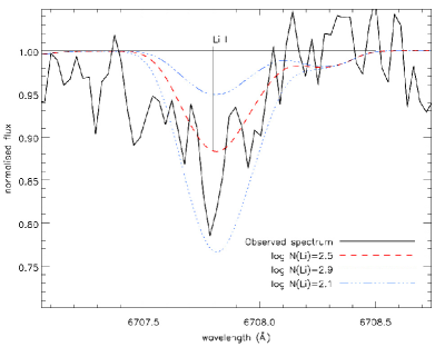
Figure 5: High-resolution HET stacked spectrum (black full line) of the WTS-1 Li i line at $\sim$6707 Å in comparison with three synthetic spectra calculated with the final adopted stellar parameters and lithium abundances ($\log$ N(Li)) of 2.5 (red dashed line), 2.9 (blue dotted line), and 2.1 (blue dash-dotted line). The vertical line indicates the position of the centre of the multiplet.

3.1.3 Properties of the host star WTS-1

The atmospheric parameters of the star WTS-1 were computed combining the results coming from the analysis described in the previous sections. We finally obtained an effective temperature of 6250$\pm$200 K, a surface gravity of 4.4$\pm$0.1 and a metallicity range $-0.5\div 0.0$ dex. As described in Section 3.1.2, the faintness of the star and the reduction process led to a distortion of the stronger lines in the HET high resolution spectrum, reducing the number of reliable lines employed in the measure of the metallicity. For these reasons, the relative uncertainty on the metallicity is larger with respect to those of the other parameters. Further observations would be needed to pin down the exact value of the star metallicity.

In order to determine the parameters of the stellar companion, mass and radius of the host star must be known. The fit of the transit in the light curves provides important constrains on the mean stellar density (see Section 3.2.1). Joining this quantity to the effective temperature, we could place WTS-1 in the modified $\rho_{s}^{-1/3}$ vs. $T_{\rm{eff}}$ H-R diagram and compare its position with evolutionary tracks and isochrones models (Girardi et al., 2000) in order to estimate stellar mass and age. In this way, we estimated the stellar mass to be 1.2$\pm$0.1 $M_{\odot}$ and the age of the system to range between 200 Myr and 4.5 Gyr.

Further constrains on the stellar age can be fixed considering the measured Li i line abundance. Depletion of lithium in stars hotter than the Sun is thought to be due to a not yet clearly identified slow mixing process during the main-sequence evolution, because those stars do not experience pre-main sequence depletion (Martín, 1997). Comparison of the lithium abundance of WTS-1 ($\log$ N(Li)=2.5$\pm$0.4) with those of open clusters rise the lower limit on the age to 600 Myr, because younger clusters do not show lithium depletion in their late-F members (Sestito & Randich, 2005). On the other hand, it is not feasible to derive an age constrain from the WTS-1 rotation rate (v $sin(i)$=7$\pm$2 km s^-1) because stars with spectral types earlier than F8 show no age-rotation relation (Wolff et al., 1986) and thus they are left out from the formulation of the spin down rate of low-mass stars (Stepién, 1988).

The true space motion knowledge of WTS-1 allows to determine to which component of our Galaxy it belongs. In order to compute the U, V and W components of the motion, the following set of quantities was required: distance, systemic velocity (from the RV fit, see Section 3.2.2), proper motion (from SDSS $7^{th}$ release, Munn et al., 2004, 2008) and coordinates of the star. The distance to the observed system was estimated according to the extinction, fitted in the SED analysis (A_V=$0.44\pm 0.07$), and a model of dust distribution in the galaxy (Amôres & Lépine, 2005, axis-symmetric model). The UVW values and their errors are calculated using the method in Johnson & Soderblom (1987), with respect to the Sun (heliocentric) and in a left-handed coordinate system, so that they are positive away from the Galactic centre, Galactic rotation and the North Galactic Pole respectively. All the quantities here discussed are listed in Table 5. Considering the uncertainties on the derived quantities, maily affected by the error on the distance, the host star is consistent with both the definitions of Galactic young-old disk and young disk populations (metallicity between -0.5 and 0 dex, solar-metallicity respectively, Leggett, 1992). But we could assess that WTS-1 is not a halo member.

Combining $\rho_{s}$ and M_s, a value of $1.15^{+0.10}_{-0.12}$ $R_{\odot}$ was computed for the stellar radius. The same result was obtained considering the stellar mass and the surface gravity measured from the spectroscopic analysis. Scaling by the distance the apparent $V$ magnitude calculated from the SDSS $g$ and $r$ magnitudes (Jester et al., 2005), we computed an absolute $V$ magnitude of $3.55^{+0.27}_{-0.38}$. This value and all the other derived stellar parameters are consistent with each other and with the typical quantities expected for an F6-8 main-sequence star (Torres et al., 2009). They are collected in Table 5.

Table 5: Properties of the WTS-1 host star.

[b] Parameter Value $T_{\rm{eff}}$ 6250$\pm$200 K log $g$ 4.4$\pm$0.1 $[\rm{Fe/H}]$ [-0.5, 0] dex M_s 1.2$\pm$0.1 $M_{\odot}$ R_s $1.15^{+0.10}_{-0.12}$ $R_{\odot}$ m_V 16.13$\pm$0.04 M_V $3.55^{+0.27}_{-0.38}$ v $sin(i)$^a 7$\pm$2 km s^-1 $\rho_{s}$ $0.79^{+0.31}_{-0.18}$ $\rho_{\rm{sun}}$ Age [0.6, 4.5] Gyr Distance $3.2^{+0.9}_{-0.4}$ kpc True space motion U^c 13$\pm$28 km s^-1 True space motion V^c 20$\pm$38 km s^-1 True space motion W^c -12$\pm$26 km s^-1

• We assumed $v_{mic}$=0.85 km s^-1;

• Epoch J2000;

• Left-handed coordinates system (see text).

3.2 Planetary parameters

3.2.1 Transit fit

The light curves in $J$- and $i^{\prime}$-band were fitted with analytic models presented by Mandel & Agol (2002). We used quadratic limb-darkening coefficients for a star with effective temperature $T_{\rm{eff}}$=6250 K, surface gravity log $g$=4.4 and metallicity $[\rm{Fe/H}]$=-0.5 dex, calculated as linear interpolations in $T_{\rm{eff}}$, log $g$ and $[\rm{Fe/H}]$ of the values tabulated in Claret & Bloemen (2011). We use their table derived from ATLAS atmospheric models using the flux conservation method (FCM) which gave a slightly better fit than the ones derived using the least-squares method (LSM). The values of the limb-darkening coefficients we used in our fitting are given in Table 6. Scaling factors were applied to the error values of the $J$- and $i^{\prime}$-band light curves (0.94 and 0.9 respectively) in order to achieve a reduced $\chi^{2}$ of the constant out-of-transit part equal to 1.

Using a simultaneous fit to both light curves, we fitted the period $P$, the time of the central transit t₀, the radius ratio $R_{\rm{p}}/R_{\rm{s}}$, the mean stellar density, $\rho_{s}=M_{\rm{s}}/R^{3}_{\rm{s}}$ in solar units and the impact parameter $\beta_{\rm{impact}}$ in units of $R_{\rm{s}}$. The light curves and the model fit are shown in Figures 6 and 7, while the resulting parameters are listed in Table 7.

Table 6: Quadratic limb-darkening coefficients used for the transit fitting, for a star with effective temperature $T_{\rm{eff}}$=6250 K, surface gravity log $g$=4.4 and metallicity $[\rm{Fe/H}]$=-0.5 dex (Claret & Bloemen, 2011).

filter	$\gamma_{1}$	$\gamma_{2}$
J	0.14148	0.24832
i′	0.25674	0.26298

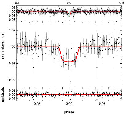
Figure 6: WFCAM J-band light curve data of WTS-1. $Upper$ $panel$: whole set of the folded WFCAM J-band data points. $Middle$ $panel$: folded photometric data centred in the transit and best model (red line) fitted in combination with the INT i^′-band data. $Lower$ $panel$: residuals of the best fit.

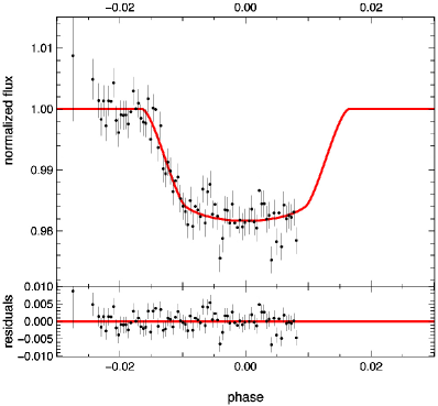
Figure 7: INT $i^{\prime}$-band light curve data of WTS-1. $Upper$ $panel$: photometric data and best model (red line) fitted in combination with the WFCAM $J$-band data. $Lower$ $panel$: residuals of the best fit.

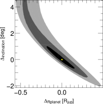
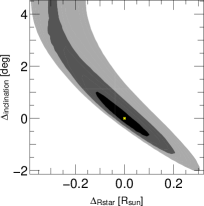
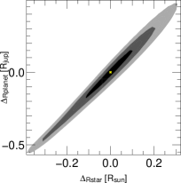
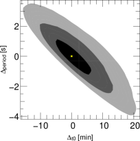
Figure 8: Correlation plots of the quantities derived from the simultaneous fit of the transit in the $J$ and $i^{\prime}$-band light curves. The $\chi^{2}$ minima are indicated by crosses while the different tones of grey correspond to the 68$\%$, 95$\%$ and 99$\%$ confidence level (darker to lighter respectively). The other couples of parameters do not show significant correlations.

The errors were calculated using a multi-dimensional grid on which we search for extreme grid points with $\Delta\chi^{2}$=1 when varying one parameter and simultaneously minimizing over the others. Figure 8 shows the correlations between the parameters of the WTS-1 system derived from the simultaneous fit of the $J$- and $i^{\prime}$-band light curves. Considering the solar metallicity scenario, with different limb-darkening coefficients, the change in the final fitting parameters is smaller than 1% of their uncertainties. Note that the combined fit assumes a fixed radius ratio although in a hydrogen-rich atmosphere, molecular absorption and scattering processes could result in different radius ratios in each band (an attempt to detect such variations has recently been undertaken by de Mooij et al., 2012). In our case, the uncertainties are too large to see this effect in the light curves and the assumption of a fixed radius ratio is a good approximation. The estimated stellar density of the host star ($0.79^{+0.31}_{-0.18}$ $\rho_{\rm{sun}}$) is consistent with the expected value based on its spectral type (Seager & Mallen-Ornelas, 2003). The noise in the data did not allow a secondary transit detection.

Subsequently, we searched for further periodic signals in the light curve after the removal of the data points related to the transit. No significant signals were detected in the Lomb-Scargle periodogram up to a period of 400 days. Since WTS-1 is a late F-star, there are not many spots on the surface and they do not live long enough to produce a stable signal over a timescale of several years.

Table 7: Fitted parameters of the WTS-1 system as determined from the simultaneous fit of the $J$- and $i^{\prime}$-band light curves. Scaling factors to the uncertainties of the $J$ and $i^{\prime}$ data points (0.94 and 0.9 respectively) were applied in order to achieve a reduced $\chi^{2}$=1 in the constant out-of-transit part of the light curves.

Parameter		Value
$P_{orb}$	=	$3.352059^{+1.2\times 10^{-5}}_{-1.4\times 10^{-5}}$ days
t0	=	2 454 318.7472${}^{+0.0043}_{-0.0036}$ HJD
Rp/Rs	=	$0.1328^{+0.0032}_{-0.0035}$
$\rho_{s}$	=	$0.79^{+0.31}_{-0.18}$ $\rho_{\rm{sun}}$
$\beta_{\rm{impact}}$	=	$0.69^{+0.05}_{-0.09}$

3.2.2 Radial velocity

One of the most pernicious transit mimics in the WTS are eclipsing binaries. On one hand, a transit can be mimicked by an eclipsing binary that is blended with foreground or background star. On the other hand, grazing eclipsing binaries with near-equal radius stars also have shallow, near-equal depth eclipses that can phase-fold into transit-like signals at half the binary orbital period. In order to rule out the eclipsing binaries scenarios, the RV variation of the WTS-1 system were first measured using the ISIS/WHT intermediate resolution spectra. Eclipsing binaries systems typically show RV amplitudes of tens of km s^-1, while the measured RVs were all consistent with a flat trend within the RV uncertainties of $\sim 1$ km s^-1.

Table 8: Radial velocities and bisector spans measurements for WTS-1 obtained by HET spectra. The phases were computed from the epochs of the observations expressed in Julian date and using the $P$ and $t_{0}$ values found with the transit fit.

HJD	Phase	RV	BS
-2 400 000		[km s-1]	[km s-1]
55477.676	0.74	$-1.46\pm 0.12$	$-0.31\pm 0.40$
55479.666	0.33	$-1.80\pm 0.10$	$-0.77\pm 0.39$
55499.608	0.28	$-2.03\pm 0.10$	$0.76\pm 0.51$
55513.586	0.45	$-2.06\pm 0.17$	$0.87\pm 0.63$
55522.556	0.13	$-2.09\pm 0.44$	$-0.39\pm 0.35$
55523.542	0.42	$-1.70\pm 0.16$	$-0.13\pm 0.44$
55742.729	0.26	$-1.97\pm 0.15$	$0.27\pm 0.68$
55760.673	0.79	$-1.11\pm 0.12$	$-0.47\pm 0.59$
55782.837	0.22	$-2.23\pm 0.07$	$0.41\pm 0.39$
55824.722	0.25	$-2.31\pm 0.06$	$0.16\pm 0.56$
55849.650	0.75	$-1.19\pm 0.06$	$0.18\pm 0.31$

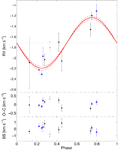
Figure 9: $Top$ $panel$: RVs values measured with the high-resolution HET spectra of WTS-1 as a function of the orbital phase. Black dots and blue triangles refers to observations performed in 2010 and 2011 respectively. The data point at $\phi=0.33$, empty dot, was excluded from the fitting procedure (see text for details). Best-fit circular orbit model ($\chi^{2}_{\nu}$=1.45) and 1$\sigma$ uncertainty of the semi-amplitude ($K_{\star}$=479$\pm$34 m s^-1) are indicated with solid and dashed red lines respectively. The black dotted line refers to the fitted radial systemic velocity ($\gamma$=-1 714$\pm$35 m s^-1). Zero phase corresponds to the mid-transit time. $Middle$ $panel$: Phase folded O-C residuals from the best-fit. The residual scatter is of the order of $\sim 150$ m s^-1, consistent with the RVs uncertainties. $Bottom$ $panel$: Bisector spans. No significant deviations from zero and no correlation with the RVs were found.

Afterwards, we analysed the high-resolution HET spectra in order to accurately investigate the properties of the sub-stellar companion of WTS-1. The spectra related to each single night were cross-correlated using the iraf.rv.fxcorr task with the synthetic spectrum of a star with $T_{\rm{eff}}$=6250 K, log $g$=4.4 and $[\rm{Fe/H}]$=-0.5. Changes in the effective temperature of the synthetic templates, even of the order of several hundreds of Kelvin, cause variations of the measured RV values smaller than the statistical uncertainties due to noise in the spectra (suggesting the absence of contamination of back/foreground stars of different spectral type). Even smaller variations occur changing surface gravity and metallicity of the template. The 40 single RV values, each one coming from a different order, were used to compute the RVs and related uncertainty at each epoch of the observations. Resampling statistical tools were used in order to better estimate mean value, standard deviation and possible bias in the sample of measured RVs. Finally, the measured RVs were corrected for the Earth orbital movements and reduced to the heliocentric rest-of-frame. The phase values $\phi$ were computed from the epochs of the observations, expressed in Julian date, and using the extremely well determined $P$ and $t_{0}$ values (relative uncertainties are of the order of $10^{-6}$ and $10^{-9}$ respectively) obtained from the photometric fit (see Table 7).

The data, listed in Table 8, were then fitted with a simple two parameters sinusoid of the form:

$$RV=\gamma+K_{\star}sin(2\pi\phi)$$ (1)

where $K_{\star}$ is the RV semi-amplitude of the host star and $\gamma$ is the systemic velocity of the system. Thanks to the acquisition of two ThAr calibration exposures (before and after the science exposure, see Section 2.2.4), we detected a small drift between the ThAr lines occurring during the science exposures on November 22, 2010. In the presence of a suspected systematic trend, which could affect the measured RV value, we performed the fitting procedure excluding the data point related to that night (at $\phi=0.33$). The larger RV error of the data point at $\phi=0.13$ is due to the integration time (half hour) of the science frame which is shorter than those of all the other data points (one hour). The best fitting model ($\chi^{2}_{\nu}$=1.45) was obtained for $K_{\star}$=479$\pm$34 m s^-1and $\gamma$=-1 714$\pm$35 m s^-1and is plotted in Figure 9 with the RV data. We imposed the orbit to be circular as the eccentricity was compatible with zero when a Keplerian orbit fit was performed (see Anderson et al. (2012) for a discussion of the rationale for this). In accordance to the RV uncertainties, a relatively loose upper limit can be plaved on the eccentricity ($e<0.1$, C.L.$=95\%$). The fitted RV semi-amplitude implies a planet mass of 4.01$\pm$0.35 $M_{J}$  assuming a host star mass of 1.2$\pm$0.1 $M_{\odot}$ (see Section 3.1.3). The uncertainty on the planet mass in mainly driven by the uncertainty on the mass of the host star. As can be seen in Figure 9, the RVs related to observations performed in late 2010 and in the second half of 2011 are consistent, showing no significant long term trends in our measurements.

The HET spectra were employed also to investigate the possibility that the measured RVs are not due to true Doppler motion in response to the presence of a planetary companion. Similar RV variations can rise in case of distortions in the line profiles due to stellar atmosphere oscillations (Queloz et al., 2001). To assert that this is not our case, we used the same cross-correlation profiles produced previously for the RV calculation to compute the bisector spans (BS hereafter) which are reported in Table 8. Following Torres et al. (2005), we measured the difference between the bisector values at the top and at the bottom of the correlation function for the different observation epochs. In case of contaminations, we would have expected to measure BS values consistently different from zero and a strong correlation with the measured RVs (Queloz et al., 2001; Mandushev et al., 2005). As it can be seen in the bottom panel of Figure 9, the measured BS do not show significant deviation from zero within the uncertainties. No correlation was detected between the BS and the RV values. In this way, contaminations that could mimic the effect of the presence of a planet were ruled out.

4 Discussion and conclusions

Table 9: Properties of the new extrasolar planet WTS-1b.

[b] Parameter Value M_p 4.01$\pm$0.35 $M_{J}$ R_p $1.49^{+0.16}_{-0.18}$ $R_{J}$ $P_{rot}$ $3.352057^{+1.3\times 10^{-5}}_{-1.5\times 10^{-5}}$ d a 0.047$\pm$0.001 AU e $<0.1$ (C.L.$=95\%$) inc $85.5^{+1.0}_{-0.7}$ deg $\beta_{\rm{impact}}$ $0.69^{+0.05}_{-0.09}$ t₀ 2 454 318.7472${}^{+0.0043}_{-0.0036}$ HJD $\rho_{p}$ 1.61$\pm$0.56 $g~{}cm^{-3}$, 1.21$\pm$0.42 $\rho_{J}$ $T_{eq}$^a 1500$\pm$100 K

• We assumed a Bold albedo A_B=0 and re-irradiating fraction F$=1$;

In this paper we announce the discovery of a new transiting extrasolar planet, WTS-1b, the first detected by the UKIRT/WFCAM Transit Survey. The parameters of the planet are collected in Table 9. WTS-1b is a $\sim$4 $M_{J}$ planet orbiting in 3.35 days a late F-star with possibly slightly subsolar metallicity. With a radius of $1.49^{+0.16}_{-0.18}$ $R_{J}$, it is located in the upper part of the mass – radius diagram of the known extrasolar planets in the mass range 3-5 $M_{J}$ (see Figure 10). The parameters of the other planets are taken from www.exoplanet.eu at the time of the publication of this work. Planets with only an upper limit on the mass and/or on the radius are not shown. It is worth noting that only a cut-off of the transit depth, different for each survey, could act as a selection effect against the detection of planets in this upper portion of the diagram. Larger planetary radii imply a deeper transit feature in the light curves and thus, within this mass range, larger object are more easily detectable. The properties of WTS-1b, as well as those of the other two planets present in the upper part of the diagram, CoRoT-2b (Alonso et al., 2008) and OGLE2-TR-L9b (Snellen et al., 2009), are not explained within standard formation and evolution models of isolated gas giant planets (Guillot, 2005).

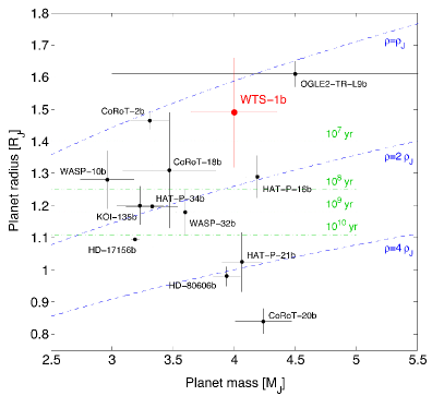
Figure 10: Mass – Radius diagram of the known planets with a mass in the range 3-5 $M_{J}$(black dots). Labels with the related planet name are shown for an easier identification. Planets with only an upper limit on mass and/or radius are not shown. The blue dashed lines represent the iso-density curves. The green dot-dashed lines indicate the planetary radii at different ages accordingly to Fortney et al. (2007) (see text for details). Masses, radii of the planets are taken from www.exoplanet.eu at the time of the publication of this work, while the related uncertainties were found in the refereed publication. WTS-1b is shown in red.

The radius anomaly is at the $\sim 2\sigma$ level considering the stellar irradiation that retards the contraction of the planets, the distance of the planet from the host star and the age of the planet (Fortney et al., 2007). The models of Fortney and collaborators predict indeed a radius of 1.2 $R_{J}$ for a 600 Myr-old planet (see their Figure 5, 3 $M_{J}$ and 0.045 AU model). This radius estimate is an upper limit as 600 Myr is the lower limit on the age of the WTS-1 system due to the Li abundance (see Section 3.1.3). The radius trend shown in the figure would suggest an age for WTS-1b less than 10 Myr. The same significance on the radius anomaly is obtained considering empirical relationships coming from the fit of the observed radii as a function of the physical properties of the star-planet system, such as mass, equilibrium temperature and tidal heating (Enoch et al., 2012, eq. 10). In any case, a rapid migration of WTS-1b inward to the highly-irradiated domain after its formation seems required.

Surface day/night temperature gradients due to the strong incident irradiation, are likely to generate strong wind activity through the planet atmosphere. Recently, Wu & Lithwick (2012) showed how the Ohmic heating proposal (Batygin & Stevenson, 2010; Perna et al., 2010) can effectively bring energy in the interior of the planet and slow down the cooling contraction of a HJ even on timescales of several Gyr: a surface wind blowing across the planetary magnetic field acts as a battery that rises Ohmic dissipation in the deeper layers. In Huang & Cumming (2012), the Ohmic dissipation in HJs is treated decoupling the interior of the planet and the wind zone. In this scenario, the radius evolution for an irradiated HJ planet (see their Figure 9, 3 $M_{J}$) leads to a value consistent with our observation up to 3 Gyr.

Accordingly to Fortney et al. (2008), the incident flux (the amount of energy from the host star irradiation, per unit of time and surface, that heats the surface of the planet) computed for WTS-1b (1.12$\pm$0.26 $\cdot$ 10⁹ erg s^-1 cm^-2) assigns it to the so called pM class of HJs. This classification considers the day-side atmospheres of the highly-irradiated HJs that are somewhat analogous to the M- and L-type dwarfs. In particular, the predictions of equilibrium chemistry for pM planet atmospheres are similar to M-dwarf stars, where absorption by TiO, VO, $H_{2}O$, and CO is prominent (Lodders, 2002). Planets in this class are warmer than required for condensation of titanium (Ti)- and vanadium (V)-bearing compounds and will possess a temperature inversion (which could lead to a smaller inflation due to Ohmic heating accordingly to Heng (2012)) due to absorption of incident flux by TiO and VO molecules. Fortney et al. (2008) propose that these planets will have large day/night effective temperature contrasts and an anomalous brightness in secondary eclipse at mid-infrared wavelengths. Unfortunately, the SNR in the $J$-band light curve, due to the faintness of the parent star WTS-1, is not high enough for such kind of detection (see Section 3.2.1).

To conclude, the discovery of WTS-1b demonstrates the capability of WTS to find planets, even if it operates in a back-up mode during dead time on a queue-schedule telescope and despite of the somewhat randomised observing strategy. Moreover, WTS-1b is an inflated HJ orbiting a late F-star even if the project is designed to search for extrasolar planets hosted by M-dwarfs. Birkby et al. 2012b will present the second WTS detection, WTS-2b, a Jupiter-like planet around a cool K-star.

References

- Aigrain & Irwin (2004) Aigrain S., Irwin M., 2004, MNRAS, 350, 331
- Alonso et al. (2008) Alonso R., Auvergne M., Baglin A., Ollivier M., Moutou C., Rouan D., Deeg H. J., Aigrain S., Almenara J. M., Barbieri M., Barge P. Benz W., Bordé P., Bouchy F., de La Reza R., Deleuil M., Dvorak R., Erikson A., Fridlund M., Gillon M., Gondoin P., Guillot T., Hatzes A., Hébrard G., Kabath P., Jorda L., Lammer H., Léger A., Llebaria A., Loeillet B., Magain P., Mayor M., Mazeh T., Pätzold M., Pepe F., Pont F., Queloz D., Rauer H., Shporer A., Schneider J., Stecklum B., Udry S., Wuchterl G., 2008, A&A, 482L, 21A
- Amôres & Lépine (2005) Amôres E. B., Lépine J. R. D., 2005, AJ, 130, 659
- Anderson et al. (2012) Anderson D. R., Collier Cameron A., Gillon M., Hellier C., Jehin E., Lendl M., Maxted P. F. L., Queloz D., Smalley B., Smith A. M. S., Triaud A. H. M. J., West R. G., Pepe F., Pollacco D., Ségransan D., Todd I., Udry S., 2012, MNRAS, 422, 1988
- Baraffe et al. (1998) Baraffe I., Chabrier G., Allard F., Hauschildt P. H., 1998, A&A, 337, 403B
- Baraffe et al. (2010) Baraffe I., Chabrier G., Barman T., 2010, arXiv, 1001, 3577
- Barbuy (1982) Barbuy B., 1982, PhD thesis, Université de Paris VII
- Barbuy et al. (2003) Barbuy B., Perrin M. N., Katz D., Coelho P., Cayrel R., Spite M., Van’t Veer-Menneret C., 2003, A&A, 404, 661
- Batygin & Stevenson (2010) Batygin K., Stevenson D. J., 2010, ApJ, 714, 238B
- Bayo et al. (2008) Bayo A., Rodrigo C., Barrado y Navascués D., Solano E., Gutiérrez R., Morales-Calderón M., Allard F., 2008, A&A, 492, 277B
- Bayo et al. (2012) Bayo A., submitted, 2012
- Birkby et al. (2011) Birkby J., Hodgkin S., Pinfield D., WTS consortium, 2011, ASPC, 448, 803B
- Birkby et al. (2012a) Birkby J., Nefs B., Hodgkin S., Kovács G., Sipőcz B., Pinfield D., Snellen I., Mislis D., Murgas F., Lodieu N., de Mooij E., Goulding N., CruzP., Stoev h., Cappetta M., Palle E., Barrado D., Saglia R. P., Martín E., Pavlenko Y., 2012a, MNRAS accepted, arXiv, 1206, 2773B
- Birkby et al. (2012b) Birkby et al. 2012b,
- Bodenheimer et al. (2001) Bodenheimer P., Lin D. N. C., Mardling R. A., 2001, ApJ, 548, 466B
- Bodenheimer et al. (2003) Bodenheimer P., Laughlin G., Lin D. N. C., 2003, ApJ, 592, 555B
- Burrows et al. (2007) Burrows A., Hubeny I., Budaj J., Hubbard W. B., 2007, ApJ, 661, 502B
- Cayrel et al. (1991) Cayrel R., Perrin M. N., Barbuy B., Buser R., 1991, A&A, 247, 108
- Canuto & Mazzitelli (1991) Canuto V. M., Mazzitelli I., 1991, ApJ, 370, 295C
- Casali et al. (2007) Casali M., Adamson A., Alves de Oliveira C., Almaini O., Burch K., Chuter T., Elliot J., Folger M., Foucaud S., Hambly N., Hastie M., Henry D., Hirst P., Irwin M., Ives D., Lawrence A., Laidlaw K., Lee D., Lewis J., Lunney D., McLay S., Montgomery D., Pickup A., Read M., Rees N., Robson I., Sekiguchi K., Vick A., Warren S., Woodward B., 2007, A&A, 467, 777C
- Castelli et al. (1997) Castelli F., Gratton R.G., Kurucz R.L., 1997, A&A, 318, 841
- Castelli & Kurucz (2003) Castelli F., Kurucz R.L., 1997, Modelling of Stellar Atmospheres, 210, 20P
- Chabrier et al. (2007) Chabrier G., Baraffe I., 2007, ApJ, 661L, 81C
- Claret & Bloemen (2011) Claret A., Bloemen S., 2011, A&A, 529, 75
- Coelho et al. (2005) Coelho P., Barbuy B., Meléndez J., Schiavon R. P., Castilho B. V., 2005, A&A, 443, 735C
- Collier Cameron et al. (2007) Collier Cameron A., Wilson D. M., West R. G., Hebb L., Wang X. B., Aigrain S., Bouchy F., Christian D. J., Clarkson W. I., Enoch B., Esposito M., Guenther E., Haswell C. A., Hébrard G., Hellier C., Horne K., Irwin J., Kane S. R., Loeillet B., Lister T. A., Maxted P., Mayor M., Moutou C., Parley N., Pollacco D., Pont F., Queloz D., Ryans R., Skillen I., Street R. A., Udry S., Wheatley P. J., 2007, MNRAS, 380, 1230
- Covey et al. (2007) Covey K. R., Ivezić Ž., Schlegel D., Finkbeiner D., Padmanabhan N., Lupton R. H., Agüeros M. A., Bochanski J. J., Hawley S. L., West A. A., Seth A., Kimball A., Gogarten S. M., Claire M., Haggard D., Kaib N., Schneider D. P., Sesar B., 2007, AJ, 134, 2398
- Demory & Seager (2011) Demory B. O., Seager S., 2011, ApJS, 197, 12D
- Enoch et al. (2012) Enoch B., Collier Cameron A., Horne K., 2012, A&A, 540, 99
- Fossati et al. (2009) Fossati L., Ryabchikova T., Bagnulo S., Alecian E., Grunhut J., Kochukhov O., Wade G., 2009, AAP, 503, 945
- Fossati et al. (2011) Fossati L., Ryabchikova T., Shulyak D. V., Haswell C. A., Elmasli A., Pandey C. P., Barnes T. G., Zwintz K. 2011, MNRAS, 417, 495
- Fortney et al. (2007) Fortney J. J., Marley M. S., Barnes J. W., 2007, ApJ, 659, 1661
- Fortney et al. (2008) Fortney J. J., Lodders K., Marley M. S., Freedman R. S., 2008, ApJ, 678, 1419
- Fuhrmann et al. (1993) Fuhrmann K., Axer M., Gehren T., 1993, AAP, 271, 451
- Girardi et al. (2000) Girardi L., Bressan A., Bertelli G., Chiosi C., 2000, A&AS, 141, 371G
- Goulding et al. (2012) Goulding N. T., et al., 2012, in prep.
- Guillot (2005) Guillot T., 2005, Ann Rev EPS, 33, 493G
- Heng (2012) Heng K., 2012, ApJ, 748, L17
- Hodgkin et al. (2009) Hodgkin S. T., Irwin M. J., Hewett P. C., Warren S. J., 2009, MNRAS, 394, 675H
- Huang & Cumming (2012) Huang X., Cumming A., 2012, arXiv, 1207, 3278
- Irwin et al. (2007) Irwin J., Irwin M., Aigrain S., Hodgkin S., Hebb L., Moraux E., 2007, MNRAS, 375, 1449I
- Irwin & Lewis (2001) Irwin M., Lewis J., 2001, New Astronomy Reviews, 45, 105
- Jackson et al. (2008) Jackson B., Greenberg R., Barnes R., 2008, ApJ, 678, 1396J
- Jester et al. (2005) Jester S., Schneider D. P., Richards G. T., Green R. F., Shmidt M., Hall P. B., Strauss M. A., Vanden Berk D. E., Stoughton C., Gunn J. E., Brinkmann J., Kent S. M., Smith J. A., Tucker D. L., Yanny B., 2005, AJ, 130, 873J
- Johnson & Soderblom (1987) Johnson D. R. H., Soderblom D. R., 1987, AJ, 93, 864
- Kochukhov (2007) Kochukhov O., 2007, Spectrum synthesis code SYNTH3
- Kovács et al. (2012) Kovács B., Hodgkin S., Sipőcz B., Pinfield D., Barrado D., Birkby J., Cappetta M., Cruz P., Koppenhöfer J., Martín E., Murgas F., Nefs B., Saglia R. P., Zendejas J., 2012, MNRAS submitted
- Kupka et al. (1999) Kupka F., Piskunov N., Ryabchikova T. A., Stempels H. C., Weiss W. W., 1999, A&AS, 138, 119
- Kurucz (1993) Kurucz R. L., 1993, Stells surface structure, 523
- Leconte & Chabrier (2012) Leconte J., Chabrier G., 2012, A&A, 540A, 20L
- Laughlin et al. (2010) Laughlin G., Crismani M., Adams F. C., 2011, ApJ, 729, 7
- Leggett (1992) Leggett S. K., 1992, ApJSS, 82, 351
- Lodders (2002) Lodders K., ApJ, 577, 974L
- Liu, Burrows & Ibgui (2008) Liu X, Burrows A., Ibgui L., 2008, ApJ, 687, 1191L
- Lin et al. (1996) Lin D. N. C., Bodenheimer P., Richardson D. C., 1996, Nature, 380, 606L
- McMahon et al. (2001) McMahon R. G., Walton N. A., Irwin M. J., Lewis J. R., Bunclark P. S., Jones D. H., 2001, New Astronomy Reviews, 45, 97
- Mandel & Agol (2002) Mandel K., Agol E., 2002, ApJ, 580L, 171M
- Mandushev et al. (2005) Mandushev G., Torres G., Latham D. W., Charbonneau D., Alonso R., White R.Y., Stefanik R. P., Dunham E. W., Brown T.M., O’Donovan F. T., 2005, ApJ, 621, 1061
- Martín (1997) Martín E. L., 1997, A&A, 321, 492
- Martín et al. (2011) Martín E. L., Spruit H. C., Tata R., 2011, A&A, 535A, 50M
- Mashonkina (2011) Mashonkina L., 2011, mast.conf, 314M
- de Mooij et al. (2012) de Mooij E. J. W., Brogi M., de Kok R. J., Koppenhöefer J., Nefs S. V., Snellen I. A. G., Greiner J., Hanse J., Heinsbroek R. C., Lee C. H., van der Werf P. P., 2012, A&A, 538, 46
- Munn et al. (2004) Munn J. A., Monet D. G., Levine S. E., Canzian B., Pier J. R., Harris H. C., Lupton R. H., Ivezí Z., Hindsley R. B., Hennessy G. S., Schneider D. P.k Brinkmann J., 2004, AJ, 127, 3034M
- Munn et al. (2008) Munn J. A., Monet D. G., Levine S. E., Canzian B., Pier J. R., Harris H. C., Lupton R. H., IveziŹ., Hindsley R. B., Hennessy G. S., Schneider D. P.k Brinkmann J., 2008, AJ, 136, 895M
- Nash (1996) Nash T., 1996, sube.conf, 477N
- Perna et al. (2010) Perna, R., Menou, K., Rauscher, E. 2010, ApJ, 724, 313
- Piskunov et al. (1995) Piskunov N. E., Kupka F., Ryabchikova T. A., Weiss W. W., Jeffery C. S., 1995, A&AS, 112, 525P
- Pont et al. (2006) Pont F., Zucker S., Queloz D., 2006, MNRAS, 373, 231
- Queloz et al. (2001) Queloz D., Henry G. W., Sivan J. P., Baliunas S. L., Beuzit J. L., Donahue R. A., Mayor M., Naef D., Perrier C., Udry S., 2001, A&A, 379, 279
- Ramsey et al. (1998) Ramsey L. W., Adams. M. T., Barnes T. G., Booth J. A., Cornell M. E., Fowler J. R., Gaffney N. I., Glaspey J. W., Good J. M., Hill G. J., Kelton P. W., Krabbendam V. L., Long L., MacQueen P. J., Ray F. B., Ricklefs R. L., Sage J., Sebring T. A., Spiesman W. J., Steiner M., 1998, SPIE, 3352, 34
- Rosman & Taylor (1998) Rosman K. J. R. & Taylor P. D. P. 1998, Journal Phys. Chem. Ref. Data, 27, 1275
- Ryabchikova et al. (1999) Ryabchikova T., Piskunov N., Savanov I., Kupka F., Malanushenko V., 1999, A&A, 343, 229R
- Ryabchikova et al. (2009) Ryabchikova T. A., Fossati L., Shulyak D. V., 2009, AAP, 506, 203
- Seager & Mallen-Ornelas (2003) Seager S., Mallen-Ornelas G., 2003, ApJ, 585, 1038
- Seager et al. (2007) Seager S., Kuchner M., Hier-Majumder C. A., Militzer B., 2007, ApJ, 669, 1279S
- Sekiguchi & Fukugita (2000) Sekiguchi M., Fukugita M., 2000, AJ, 120, 1072S
- Sestito & Randich (2005) Sestito, P. & Randich, S. 2005, A&A, 442, 615
- Showman & Guillot (2002) Showman A. P., Guillot T., 2002, A&A , 385, 166
- Shulyak et al. (2004) Shulyak D., Tsymbal V., Ryabchikova T., Stütz Ch., Weiss W. W., 2004, A&A, 428, 993S
- Sipőcz et al. (2012) Sipőcz B., et al., 2012, in prep.
- Skrutskie et al. (2006) Skrutskie M. F., Cutri R. M., Stiening R., Weinberg M. D., Schneider S., Carpenter J. M., Beichman C., Capps R., Chester T., Elias J., Huchra J., Liebert J., Lonsdale C., Monet D. G., Price S., Seitzer P., Jarrett T., Kirkpatrick J. D., Gizis J. E., Howard E., Evans T., Fowler J., Fullmer L., Hurt R., Light R., Kopan E. L., Marsh K. A., McCallon H. L., Tam R., Van Dyk S. and Wheelock S., 2006, AJ, 131, 1163
- Snellen et al. (2009) Snellen I. A. G., Koppenhöefer J., van der Burg R. F. J., Dreizler S., Greiner J., de Hoon M. D. J., Husser T. O., Krühler T., Saglia R. P., Vuijsje F. N., 2009, A&A, 497, 545
- Stepién (1988) Stepién K., 1988, ApJ, 335, 907
- Torres et al. (2005) Torres G., Konacki M., Sasselov D. D., Jha S., 2005, ApJ, 619, 558
- Torres et al. (2009) Torres G., J. Andersen, A. Giménez, 2009, A&A, 18, 67
- Tsymbal (1996) Tsymbal V., 1996, ASPC, 108, 198T
- Tull (1998) Tull R. G., 1998, SPIE, 3355, 387
- Valenti & Fisher (2005) Valenti J. and Fischer D. A., 2005, ApJ, 622, 1102
- Vogt et al. (1994) Vogt S. S., Allen S. L., Bigelow B. C., Bresee L., Brown B., Cantrall T., Conrad A., Couture M., Delaney C., Epps H. W., Hilyard D., Hilyard D. F., Horn E., Jern N., Kanto D., Keane M. J., Kibrick R. I., Lewis J. W., Osborne J., Pardeilhan G. H., Pfister T., Ricketts T., Robinson L. B., Stover R. J., Tucker D., Ward J., Wei M. Z., 1994, SPIE, 2198, 362V
- Willmarth & Barnes (1994) Willmarth D., Barnes J., A user’s guide to reducing Echelle spectra with IRAF, 1994
- Wolff et al. (1986) Wolff S. C., Boesgaard A. M., Simon T., 1986, ApJ, 310, 360
- Wright et al. (2010) Wright E. L., Eisenhardt P. R. M., Mainzer A. K., Ressler M. E., Cutri R. M., Jarrett T., Kirkpatrick J. D., Padgett D., McMillan R. S., Skrutskie M., Stanford S. A., Cohen M., Walker R. G., Mather J. C., Leisawitz D., Gautier T. N., McLean I., Benford D., Lonsdale C. J., Blain A., Mendez B., Irace W. R., Duval V., Liu F., Royer D., Heinrichsen I., Howard J., Shannon M., Kendall M., Walsh A. L., Larsen M., Cardon J. G., Schick S., Schwalm M., Abid M., Fabinsky B., Naes L., Tsai C., 2010, AJ, 140, 1868
- Wu & Lithwick (2012) Wu Y., Lithwick Y., 2012, arXiv, 1202, 0026
- Youdin & Mitchell (2010) Youdin A. N., Mitchell J. L., 2010, ApJ, 721, 1113Y
- Zapolsky & Salpeter (1969) Zapolsky H. S., Salpeter E. E., 1969, ApJ…158..809Z