Evidence for a non-universal Kennicutt-Schmidt relationship using hierarchical Bayesian linear regression

Abstract

For investigating the relationship between the star formation rate and gas surface density, we develop a Bayesian linear regression method that rigorously treats measurement uncertainties and accounts for hierarchical data structure. The hierarchical Bayesian method simultaneously estimates the intercept, slope, and scatter about the regression line of each individual subject (e.g. a galaxy) and the population (e.g. an ensemble of galaxies). Using synthetic datasets, we demonstrate that the method accurately recovers the underlying parameters of both the individuals and the population, especially when compared to commonly employed ordinary least squares techniques, such as the bisector fit. We apply the hierarchical Bayesian method to estimate the Kennicutt-Schmidt (KS) parameters of a sample of spiral galaxies compiled by Bigiel et al. (2008). We find significant variation in the KS parameters, indicating that no single KS relationship holds for all galaxies. This suggests that the relationship between molecular gas and star formation differs from galaxy to galaxy, possibly due to the influence of other physical properties within a given galaxy, such as metallicity, molecular gas fraction, stellar mass, and/or magnetic fields. In four of the seven galaxies the slope estimates are sub-linear, especially for M51, where unity is excluded at the $2\sigma$ level. We estimate the mean index of the KS relationship for the population to be 0.84, with $2\sigma$ range [0.63, 1.0]. For the galaxies with sub-linear KS relationships, a possible interpretation is that CO emission is tracing some molecular gas that is not directly associated with star formation. Equivalently, a sub-linear KS relationship may be indicative of an increasing gas depletion time at higher surface densities, as traced by CO emission. The hierarchical Bayesian method can account for all sources of uncertainties, including variations in the conversion of observed intensities to star formation rates and gas surface densities (e.g. the $X_{\rm CO}$ factor), and is therefore well suited for a thorough statistical analysis of the KS relationship.

1 Introduction

1.1 The Kennicutt-Schmidt relationship

Accurately measuring the properties of star formation is crucial for understanding a variety of astrophysical topics, including the interstellar medium (ISM), galaxy structure and dynamics, and the evolution of the universe as a whole. Observations have revealed strong power-law correlations between the star formation rate $\Sigma_{\rm SFR}$ and gas surface densities in disk galaxies, now referred to as the Schmidt or Kennicutt-Schmidt (hereafter KS) law (Schmidt, 1959; Kennicutt, 1989, 1998; Kennicutt & Evans, 2012). Explaining this KS law has been a major priority in the star formation research community (see e.g. Mac Low & Klessen, 2004; McKee & Ostriker, 2007; Kennicutt & Evans, 2012, and references therein).

Recent studies have indicated that much of the KS correlation is driven by the molecular component $\Sigma_{\rm mol}$:

$$\Sigma_{\rm SFR}=a\Sigma_{\rm mol}^{N},$$ (1)

using either azimuthal averages or data from individual sub-kpc regions (Rownd & Young, 1999; Wong & Blitz, 2002; Heyer et al., 2004; Kennicutt et al., 2007; Bigiel et al., 2008, 2011; Leroy et al., 2008; Rahman et al., 2011; Schruba et al., 2011). The molecular component is usually inferred through CO observations and traces much of the cold, dense gas in the ISM, because HI saturates above surface densities $\sim$10 M_⊙ pc^-2. The range in power-law indices has been estimated from  $\buildrel<\over{\sim}$ 0.9 to  $\buildrel>\over{\sim}$ 3 (see intro in Bigiel et al. 2008, and review by Kennicutt & Evans 2012), and depends on a variety of caveats, such as the observed scale, tracer, calibration of star formation rates (e.g. Calzetti et al., 2007; Rahman et al., 2011; Liu et al., 2011; Leroy et al., 2012), and a host of properties of the source, such as the metallicity, gas fractions, and stellar mass (e.g. Leroy et al., 2008; Shi et al., 2011; Saintonge et al., 2011).

Averaged over entire galaxy disks, Kennicutt (1989, 1998) found that $N$ =1.4 $\pm$ 0.15 describes the KS relationship well for over five orders of magnitude in total gas surface density (see also Buat et al., 1989). Kennicutt et al. (2007) and Liu et al. (2011) infer a similar power-law relationship on $\sim$500-2000 pc scales in the spiral galaxy M51 (NGC 5194). An interpretation for $N$=1.5 is that the dominant timescale is determined by global gravitational instability (Quirk, 1972; Kennicutt, 1989). Bigiel et al. (2008), hereafter B08, analyzed resolved observations of a sample of galaxies, and inferred an approximately linear molecular KS relationship at intermediate densities 10 M_⊙ pc^-2 $<$ $\Sigma_{\rm mol}$ $<$ 100 M_⊙ pc^-2  and speculated about a super-linear relationship at higher densities. As discussed by B08 a linear relationship may be evidence of a constant molecular gas depletion time, and that extragalactic CO observations, often averaging emission over many square kpc, are simply “counting” molecular clouds with relatively similar properties. For M51, both B08 and Blanc et al. (2009) find a sub-linear KS relationship. There are numerous differences in the observations and analysis, including reduction techniques, that may account for the discrepancies between the estimated power-law indices. Thus, a comparison between the various observational investigations is often not straightforward. We also caution that any analysis and conclusions, including those from our work here, are affected by the specific assumptions that go into data reduction or conversions from observables to physical quantities. However, with these caveats in mind, we will use the B08 data sets to illustrate the application of a hierarchical Bayesian method.

1.2 Linear regression in astrophysics

A central component of many observational investigations is the quantification of the correlation between two or more observed quantities. Typically, linear regression provides estimates of the zero-point and slope of the “best-fit” regression line between the observed data. In log-space, linear regression of the logarithm of the observed quantities provide estimates of the coefficient $C$ and index $N$ of a power-law $y=Cx^{N}$. For example, linear regression is often employed to quantify the relationship between the linewidth and sizes of molecular clouds, the luminosity and kinematic velocity of galaxies (Tully-Fisher relationship), the X-ray spectral slope and Eddington ratios of quasars, the star formation rate and gas surface density in the ISM, and a host of other topics in current astrophysical research. It is thus important to understand the limitations of common fitting methods, and, whenever possible, develop accurate regression algorithms appropriate for the given problem.

One common statistical method for fitting data is the ordinary least squares (OLS), or $\chi^{2}$ fit. An OLS fit computes the best fit line by minimizing the squared error in the residuals. As Isobe et al. (1990) show, the OLS fit can produce discrepant slope and intercept estimates depending on the classification of the “dependent” and “independent” variables. An important limitation of the OLS method is that it does not account for measurement uncertainties in the regression, resulting in biased parameter estimates (Akritas & Bershady, 1996; Weiner et al., 2006; Kelly, 2007).

Further, observational datasets are often intrinsically hierarchical, or structured, but most common statistical methods do not account for any such hierarchy. For example, consider $\Sigma_{\rm SFR}$ and $\Sigma_{\rm mol}$ in a sample of observed galaxies. A given galaxy within the survey sample will contain a number of measurements of $\Sigma_{\rm SFR}$ and $\Sigma_{\rm mol}$. If a linear regression is employed on all measurements of $\Sigma_{\rm SFR}$ and $\Sigma_{\rm mol}$ from all galaxies, then any galaxy-to-galaxy variation could be lost in the global $\Sigma_{\rm SFR}$-$\Sigma_{\rm mol}$ relationship. Moreover, the global or universal relationship estimated from a linear regression analysis on all data may be biased towards the trend from one or more galaxies, e.g. those with the largest number of $\Sigma_{\rm SFR}$$-$ $\Sigma_{\rm mol}$ pairs, or, if noise is considered, to those galaxies with the highest signal-to-noise ratios and with the tightest $\Sigma_{\rm SFR}$$-$ $\Sigma_{\rm mol}$ correlations. Here, we develop a fitting method for such hierarchical data, such that we estimate regression parameters for both the population, or group, as well as the individual relationship, allowing for an assessment of the differences between individuals within the group.

In this work, we present a method which rigorously treats measurement uncertainties, as well as estimates the scatter about the fit regression lines, two aspects which can naturally be handled in a hierarchical framework. Bayesian methods are well suited for treating problems with hierarchical structure (e.g. Gelman et al., 2004; Gelman & Hill, 2007; Kruschke, 2011). Moreover, measurement uncertainties can be rigorously treated at each level in the hierarchy, such that the estimated parameters fully account for any source of uncertainty in the modelling. Bayesian methods are becoming more common in astrophysics (Loredo, 2012), and have been employed for a number of problems, such as the correlation between mass and richness of galaxy clusters (Andreon & Hurn, 2010), binary eccentricity (Hogg et al., 2010), supernova light curves (Mandel et al., 2011), modelling dust SEDs (Kelly et al., 2012) and extinction laws (Foster et al., 2012), and turbulence in the ISM (Shetty et al., 2012), to name a few applications. Here, we introduce a general hierarchical Bayesian method for linear regression, and to illustrate its applicability we estimate the parameters of the KS relationship in local galaxies.

In the next Section, we provide an overview of hierarchical modelling, and describe the hierarchical Bayesian framework. We demonstrate the accuracy of the method on synthetic datasets in Section 3. After a brief discussion on the observational datasets in Section 4, we present results from the application of the method on the B08 observations in Section 5. In Section 6, after listing some caveats and future prospects, we offer an interpretation of our results and conclude with a summary.

2 Modelling Method

In this section, we describe the modelling method we employ to estimate the parameters of the KS relationship. As Bayesian inference is still not extensively employed in astrophysics research, we describe why it may be preferred over traditional methods. We begin by motivating hierarchical modelling, in the context of the KS law. We then provide a general description of Bayesian inference, followed by the modelling method and an outline of the fitting routine. A general introduction to Bayesian analysis can be found in Kruschke (2011). For thorough descriptions of hierarchical Bayesian methods, we refer the reader to Gelman et al. (2004) and Gelman & Hill (2007).

2.1 Motivation: hierarchical modelling with measurement error

The parameters of the Kennicutt-Schmidt (KS) relationship are governed by Equation 1, relating $\Sigma_{\rm SFR}$ and $\Sigma_{\rm mol}$. One of our primary goals is to estimate the distribution of KS parameters for a population of galaxies, e.g. the mean and dispersion in KS slopes for the galaxy population. Estimating the KS relationship requires measuring $\Sigma_{\rm SFR}$-$\Sigma_{\rm mol}$ pairs within a galaxy, and for many individual galaxies. As such, the process of estimating a universal KS relationship is intrinsically hierarchical.

Of course, the star formation properties in each galaxy will likely be influenced by physical processes that may or may not be directly associated with the surface density (e.g. Leroy et al., 2008). Local or large scale processes, for example, metallicity, magnetic fields, molecular gas fractions, turbulent levels, or rotation may all influence the star formation properties, besides $\Sigma_{\rm mol}$. Moreover, Shi et al. (2011) find that $\Sigma_{\rm SFR}$ portrays a stronger correlation with the stellar surface density compared to the gas surface density across galaxies with different morphologies. Therefore, the $\Sigma_{\rm SFR}$- $\Sigma_{\rm mol}$ relationship in different galaxies may not necessarily be expected to follow a single trend, and there may be scatter about any fit KS law as formulated by Equation 1. Indeed, uniform analyses of a sample of galaxies by B08 has resulted in a range of indices 0.84 - 1.12.

Another unavoidable caveat in fitting a model is the effect of measurement uncertainties. Measurement uncertainties can produce significant biases when fitting a model (e.g. Akritas & Bershady, 1996; Weiner et al., 2006; Kelly, 2007). These uncertainties will also contribute to the scatter about any regression line, which should be quantified during the fit. Further, there are additional sources of uncertainty in the conversion between observables (e.g., UV, IR or CO intensity) and $\Sigma_{\rm SFR}$ and $\Sigma_{\rm mol}$ needed for evaluating the KS relationship. In particular, the measurements of $\Sigma_{\rm mol}$ are strongly dependent on the adopted value of the “$X_{\rm CO}$ factor”, the conversion of CO intensity to H₂ surface density, for which recent efforts have clearly demonstrated varies with environment (see e.g. Glover & Mac Low, 2011; Shetty et al., 2011a, b; Narayanan et al., 2012; Feldmann et al., 2012a; Sandstrom et al., 2012). In this work, we focus on the estimated measurement uncertainties (e.g. due to calibration) on $\Sigma_{\rm SFR}$ and $\Sigma_{\rm mol}$ directly, though we preview future efforts where $X_{\rm CO}$ will be treated self-consistently in the modelling method.

Our goals are to estimate the parameters of the KS relationship for each individual galaxy as well as the universal values, including a rigorous treatment of uncertainties and the scatter about the regression line. On the individual galaxy level, each galaxy is considered to have its own relationship between $\Sigma_{\rm SFR}$ and $\Sigma_{\rm mol}$. The parameters governing the Kennicutt-Schmidt relationship are the power-law index $N$ and the coefficient, $A$. After transforming Equation 1 to log space, we have:

$$\log(\Sigma_{\rm SFR})=A+N\log(\Sigma_{\rm mol})+\epsilon_{\rm scat}$$ (2)

where $A=\log(a)$. The scatter about the regression line is $\epsilon_{\rm scat}$, assumed to have mean 0 and dispersion $\sigma_{\rm scat}$, which is one of the parameters to be estimated from the method.

In the evaluation of Equation 2, the parameters for each galaxy should be related to the universal values of those parameters. Under a hierarchical framework, both the individual and universal, or group, parameters are estimated simultaneously. We carry out the fit under a Bayesian framework, which is ideally suited for evaluating all the parameters of a hierarchical model.

2.2 Bayesian Inference

Bayes’ Theorem allows for the evaluation of probability ${\mathcal{P}}$ of a set of parameters $\Theta$ given the observed data ${\bf\mathcal{D}}$:

$$\mathcal{P}({\Theta|\mathcal{D}})\propto\mathcal{P}({\mathcal{D}|\Theta})\mathcal{P}(\Theta).$$ (3)

Here, $\mathcal{P}(\Theta)$ is the prior on $\Theta$, where $\Theta$ is a vector of all the parameters defining a model. The parameters making up the set $\Theta$ are described below, and includes the slope of the KS law $N$, for each individual as well as the group value. The other term on the right hand side, $\mathcal{P}({\mathcal{D}|\Theta})$, is the likelihood, which is the probability of the data given the set $\Theta$. The outcome of Bayesian inference is the posterior $\mathcal{P}({\Theta|\mathcal{D}})$, which is the probability distribution function (PDF) of the model parameters $\Theta$  given the data ${\bf\mathcal{D}}$.

The next two subsections describe the measurement and the full hierarchical model, defining the likelihood and priors. We use standard statistical notation in describing how quantities are conditionally related and their distributions. Namely, $y|x$ indicates a variable $y$ given a value of $x$. And, $y|\mu,\sigma^{2}\sim\mathcal{N}(\mu,\sigma^{2})$ denotes that $y$ is drawn from a normal distribution $\mathcal{N}$, given a mean value $\mu$ and variance $\sigma^{2}$. The mean value of a vector $x$ is denoted by $\overline{x}$. In the model, we use Gamma functions $\Gamma(s,r)$ for the distributions on the inverse of the variance, with $s$ and $r$ the shape and rate parameters.

2.3 The measurement model

Due to observational uncertainties, the measured values ${\hat{\Sigma}_{\rm mol}}$ and ${\hat{\Sigma}_{\rm SFR}}$ are related to the true values $\Sigma_{\rm mol}$ and $\Sigma_{\rm SFR}$ by

$$\log\hat{\Sigma}_{\rm SFR}=\log\Sigma_{\rm SFR}+\epsilon_{\rm SFR}$$ (4)

$$\log\hat{\Sigma}_{\rm mol}=\log\Sigma_{\rm mol}+\epsilon_{\rm mol}$$ (5)

Here, $\epsilon_{\rm SFR}$ and $\epsilon_{\rm mol}$ are the random measurement errors, assumed to have mean 0 and fixed known (or estimated) dispersion $\sigma_{\rm SFR}$ and $\sigma_{\rm mol}$, respectively.

2.4 The Hierarchical Model

For each galaxy $j$ ($j=1,2,...,J$), observations provide measurements ${\hat{\Sigma}}_{\rm mol,ij}$, ${\hat{\Sigma}}_{\rm SFR,ij}$, where $i$ ($i=1,2,...,I_{J}$) indicates individual measurements within a given galaxy $J$. Along with those measurements, we have their estimated uncertainties parametrised by $\sigma_{\rm mol,ij}$ and $\sigma_{\rm SFR,ij}$. As the desired KS parameters relate the “true” values of $\Sigma_{\rm SFR}$ with $\Sigma_{\rm mol}$, we need to estimate $\Sigma_{\rm SFR}$ and $\Sigma_{\rm mol}$ from the measurements and uncertainties. The following set of conditional probability distributions denotes the relationships between those parameters on the individual galaxy level in the hierarchy, as well as the relationship between the KS parameters and the true values of $\Sigma_{\rm mol}$ and $\Sigma_{\rm SFR}$:

$$\log\hat{\Sigma}_{\rm mol,ij}|\Sigma_{\rm mol,ij}\sim\mathcal{N}(\log\Sigma_{\rm mol,ij},\sigma^{2}_{\rm mol,ij})$$ (6)

$$\log\Sigma_{\rm mol,ij}|\overline{\Sigma}_{\rm mol,j},\overline{\sigma^{2}}_{\rm mol,j}\sim\mathcal{N}(\log\overline{\Sigma}_{\rm mol,j},\overline{\sigma^{2}}_{\rm mol,j})$$ (7)

$$\log\hat{\Sigma}_{\rm SFR,ij}|\Sigma_{\rm SFR,ij}\sim\mathcal{N}(\log\Sigma_{\rm SFR,ij},\sigma^{2}_{\rm SFR,ij})$$ (8)

$$\log\Sigma_{\rm SFR,ij}|A_{j},N_{j},\Sigma_{\rm mol,ij},\sigma^{2}_{\rm scat,j}\sim$$ (9)

$$\mathcal{N}(A_{j}+N_{j}\log\Sigma_{\rm mol,ij},\sigma^{2}_{\rm scat,j})$$

We have constructed a model using normal distributions for all the relevant parameters in the individual galaxy level. Note that Equation 9 contains the KS relationship from Equation 2. The relationships above require quantities that must be evaluated in the group level of the hierarchy, i.e., those related to the distribution of KS parameters for the galaxy population, such as $A_{j},N_{j},\sigma_{\rm scat,j}$.

For the group model, we have:

$$A_{j}\,|\,\mu_{\rm A},v_{\rm A}\sim\mathcal{N}(\mu_{\rm A},v_{\rm A})$$ (10)

$$N_{j}\,|\,\mu_{N},v_{N}\sim\mathcal{N}(\mu_{N},v_{N})$$ (11)

$$\log\overline{\Sigma}_{\rm mol,j}\,|\,\mu_{\rm mol},v_{\rm mol}\sim\mathcal{N}(\mu_{\rm mol},v_{\rm mol})$$ (12)

$$1/\overline{\sigma^{2}}_{\rm mol,j}\,|\,s_{\rm mol},r_{\rm mol}\sim\Gamma(s_{\rm mol},r_{\rm mol})$$ (13)

$$1/\sigma^{2}_{\rm scat,j}\,|\,s_{\rm scat},r_{\rm scat}\sim\Gamma(s_{\rm scat},r_{\rm scat})$$ (14)

Equations 6 $-$ 14 describe the quantities for the individuals and the population. Those quantities with subscript $j$ refer to individual galaxy properties, for instance $\overline{\Sigma}_{\rm mol,j}$ is the mean gas surface density of galaxy $j$, and $\mu_{\rm mol}$ is the mean value of the surface density for all galaxies. These equations describe how the distributions of individual parameters are derived from the group parameters. For example, the individual slopes $N_{j}$ are conditional on the group slopes and variances $\mu_{N}$ and $v_{N}$, respectively. Similarly, the distributions of the group values require assumed distributions on another level in the hierarchy.

The final hierarchical level completes the model setup. The assumed distributions of quantities in this level are the “hyperpriors” which govern the group distributions, which in turn lead to the individual parameters. We construct broad hyperpriors, as we would like to rely primarily on the data to estimate the group parameters:

$$\mu_{\rm A}\sim\mathcal{N}(0,100)$$ (15)

$$1/v_{\rm A}\sim\Gamma(0.1,0.1)$$ (16)

$$\mu_{\rm N}\sim\mathcal{N}(0,100)$$ (17)

$$1/v_{\rm N}\sim\Gamma(0.1,0.1)$$ (18)

$$\mu_{\rm mol}\sim\mathcal{N}(0,100)$$ (19)

$$1/v_{\rm mol}\sim\Gamma(0.1,0.1)$$ (20)

$$s_{\rm mol}\,|\,m_{\rm mol},d_{\rm mol}=m_{\rm mol}^{2}/d_{\rm mol}^{2}$$ (21)

$$r_{\rm mol}\,|\,m_{\rm mol},d_{\rm mol}=m_{\rm mol}/d_{\rm mol}^{2}$$ (22)

$$m_{\rm mol}\sim\Gamma(1,0.1)$$ (23)

$$d_{\rm mol}\sim\Gamma(1,0.1)$$ (24)

$$s_{\rm scat}\,|\,m_{\rm scat},d_{\rm scat}=m_{\rm scat}^{2}/d_{\rm scat}^{2}$$ (25)

$$r_{\rm scat}\,|\,m_{\rm scat},d_{\rm scat}=m_{\rm scat}/d_{\rm scat}^{2}$$ (26)

$$m_{\rm scat}\sim\Gamma(1,0.1)$$ (27)

$$d_{\rm scat}\sim\Gamma(1,0.1)$$ (28)

The hierarchical model described in Equations 6 - 28 contains all the relevant conditional dependencies and distributions to evaluate Equation 3. The hyperpriors of the group KS parameters (Eqns. 15 and 17) are normally distributed, with very large variances. These wide distributions allow the data to govern the final estimates of the PDFs of $\mu_{A}$ and $\mu_{N}$. For the variances of the individual parameters, $v_{A}$ and $v_{N}$, as well as for the scatter term, their inverses are modeled as Gamma functions, for which the estimated values are again primarily governed by the data.

The main parameters we are interested in are those that define the KS relationship, at both the individual and group levels, and the scatter term about the regression line in Equation 2: $\Theta^{\prime}=(A_{j},N_{j},\mu_{A},\mu_{N},\sigma^{2}_{\rm scat,j})$. We simply marginalize over the other parameters required for estimating the regression parameters.

Modern Markov Chain Monte Carlo (MCMC) techniques allow for efficient sampling of the full parameter space. We employ the “Gibbs sampling” method for generating random draws from the posterior. The posterior is constructed by multiplying the conditional relationships defined by Equations 6 - 28. At each step in the MCMC chain, Gibbs sampling generates a random draw from the posterior by cycling through the conditional distributions of each parameter, such that a new value of each parameter is drawn from its distribution conditional on the current values of all the other parameters and the data (see, e.g., Gelman et al., 2004). We use the JAGS software (Just Another Gibbs Sampler, Plummer, 2003) within the R programming language to carry out this analysis. In our execution, we run three seperate MCMC chains, with each chain containing 25,000 steps. With this choice of a large number of sampling steps, the convergence of parameter estimates is easily achieved. Before proceeding to evaluate this model on the observed data, we use synthetic data with known parameters to verify the accuracy of this hierarchical framework.

3 Method Testing

To test the accuracy of the method, we apply it to synthetic datasets, and compare the parameter estimates to the adopted values. As we describe below, many aspects of the model assumptions are not strictly satisfied. These discrepancies allow us to test the sensitivity of the model assumptions on the derived parameter estimates.

For our initial tests, the data are constructed to resemble the observed sample we analyze in Section 5. We construct two groups, each containing 7 individual galaxies, which is the number of galaxies in the B08 sample we analyze in the next Section. For each galaxy, we choose values for the slope, intercept, and scatter and evaluate Equation 2. The chosen slopes and intercepts are results from fitting the B08 sample: for Group A, the Bayesian inferred values from this work (Section 5), and for Group B, the bisector fits (from B08). We generate 50 log($\Sigma_{\rm mol}$) values for each galaxy, which are uniformly distributed between 0.1 and 2.2, a range comparable to log($\Sigma_{\rm mol}$) from B08. We add a value drawn from a Gaussian distribution with 0 mean and 0.1 standard deviation for the intrinsic scatter term in Equation 2. For the 50 simulated values of $\Sigma_{\rm mol}$ and $\Sigma_{\rm SFR}$ of each individual galaxy, we construct ${\hat{\Sigma}_{\rm mol}}$ and ${\hat{\Sigma}_{\rm SFR}}$ by adding noise drawn from normal distributions with zero mean and standard deviations corresponding to 25% and 50% of $\Sigma_{\rm mol}$ and $\Sigma_{\rm SFR}$. These noise levels are the estimates provided in Leroy et al. (2009) and Bigiel et al. (2010). We then fit the hierarchical model over the full range of ${\hat{\Sigma}_{\rm SFR}}$ and ${\hat{\Sigma}_{\rm mol}}$. The first four columns of Tables 1 and 2 show the intercepts, slopes, and scatter terms of the test galaxies in groups A and B, respectively. The group parameters in the last row are simply the mean values of the intercept and slopes of the individual galaxies.

3.1 Bayesian Parameter Estimates

The results of the Bayesian fit on the datasets are shown in Columns 5 $-$ 5 in Tables 1 and 2. The first four columns correspond to the individual test galaxies, indicating the adopted values of the intercepts, slopes, and scatter terms, respectively. The fifth and sixth column show the median and $2\sigma$ (95%) range in the estimated intercepts of each individual test galaxy. Similarly, the seventh and eighth column shows the estimated slopes, and its $2\sigma$ range. The last column shows the posterior median of the scatter term $\sigma_{\rm scat}$ in Equation 2 . The last row of the tables shows the adopted and estimated quantities of the group distribution.

Table 1: Adopted and Bayesian inferred parameters for Test Group A

Subject	True $A$	True $N$	True $\sigma_{\rm scat}$	Bayes $A$	Bayes $2\sigma_{A}$	Bayes $N$	Bayes $2\sigma_{N}$	Bayes $\sigma_{\rm scat}$
Test Galaxy A1	$-$2.77	0.72	0.1	$-$2.79	[$-$2.9, $-$2.7]	0.74	[0.64, 0.84]	0.12
Test Galaxy A2	$-$3.21	0.88	0.1	$-$3.23	[$-$3.4, $-$3.1]	0.86	[0.76, 0.97]	0.12
Test Galaxy A3	$-$3.18	0.89	0.1	$-$3.14	[$-$3.3, $-$3.0]	0.89	[0.79, 0.99]	0.12
Test Galaxy A4	$-$2.81	0.78	0.1	$-$2.91	[$-$3.0, $-$2.8]	0.82	[0.72, 0.92]	0.12
Test Galaxy A5	$-$2.87	0.74	0.1	$-$2.91	[$-$3.0, $-$2.8]	0.76	[0.66, 0.86]	0.12
Test Galaxy A6	$-$3.22	0.91	0.1	$-$3.13	[$-$3.3, $-$3.0]	0.87	[0.78, 0.98]	0.12
Test Galaxy A7	$-$2.82	0.92	0.1	$-$2.78	[$-$2.9, $-$2.7]	0.90	[0.80, 1.00]	0.12
Group A Parameters1	$-$2.98	0.83	0.1	$-$2.99	[$-$3.2, $-$2.7]	0.84	[0.65, 1.0]	0.12

Table 2: Adopted and Bayesian inferred parameters for Test Group B

Subject	True $A$	True $N$	True $\sigma_{\rm scat}$	Bayes $A$	Bayes $2\sigma_{A}$	Bayes $N$	Bayes $2\sigma_{N}$	Bayes $\sigma_{\rm scat}$
Test Galaxy B1	$-$2.29	0.84	0.1	$-$2.30	[$-$2.4, $-$2.2]	0.85	[0.75, 0.95]	0.12
Test Galaxy B2	$-$2.53	0.92	0.1	$-$2.56	[$-$2.7, $-$2.4]	0.91	[0.81, 1.01]	0.12
Test Galaxy B3	$-$2.15	0.96	0.1	$-$2.48	[$-$2.6, $-$2.3]	0.96	[0.86, 1.06]	0.12
Test Galaxy B4	$-$2.26	0.92	0.1	$-$2.35	[$-$2.5, $-$2.2]	0.95	[0.86, 1.05]	0.12
Test Galaxy B5	$-$2.33	1.00	0.1	$-$2.36	[$-$2.5, $-$2.2]	1.01	[0.90, 1.11]	0.12
Test Galaxy B6	$-$2.54	1.12	0.1	$-$2.45	[$-$2.6, $-$2.3]	1.08	[0.97, 1.18]	0.12
Test Galaxy B7	$-$2.12	0.95	0.1	$-$2.09	[$-$2.2, $-$2.0]	0.94	[0.84, 1.06]	0.12
Group B Parameters1	$-$2.37	0.96	0.1	$-$2.37	[$-$2.6, $-$2.1]	0.96	[0.77, 1.14]	0.12

The median of the posterior, which provides estimates of the most probable parameters, is similar to the true values. Within 95%, the posterior distributions of the slope and intercept all contain the true value. The median of the scatter term is also an accurate estimate of $\sigma_{\rm scat}$. This indicates that the hierarchical fitting has accurately recovered the true parameters. It is also evident that the PDFs of the estimated group parameters include the true values, demonstrating that the method accurately recovers both the group and individual parameters, to a high degree of accuracy.

Figures 1 and 2 show the median (gray circle) and $1\sigma$ distribution (gray contour) of the estimated slope and intercepts, along with the true value (black crosses). In all but one case, the $1\sigma$ contours for the individual parameters contains the true value. For individual Galaxies A4 and B4, the true value lies just outside the $1\sigma$ contour, but is within the $2\sigma$ interval, as indicated in Tables 1 and 2. In the hierarchical model, the Bayesian estimates of the individuals are affected by the global group parameters. This effect, called “shrinkage”, drives the overestimate of the slopes for galaxies A4 and B4 towards the group inferred value, but nevertheless the true value is contained within the $2\sigma$ confidence interval.

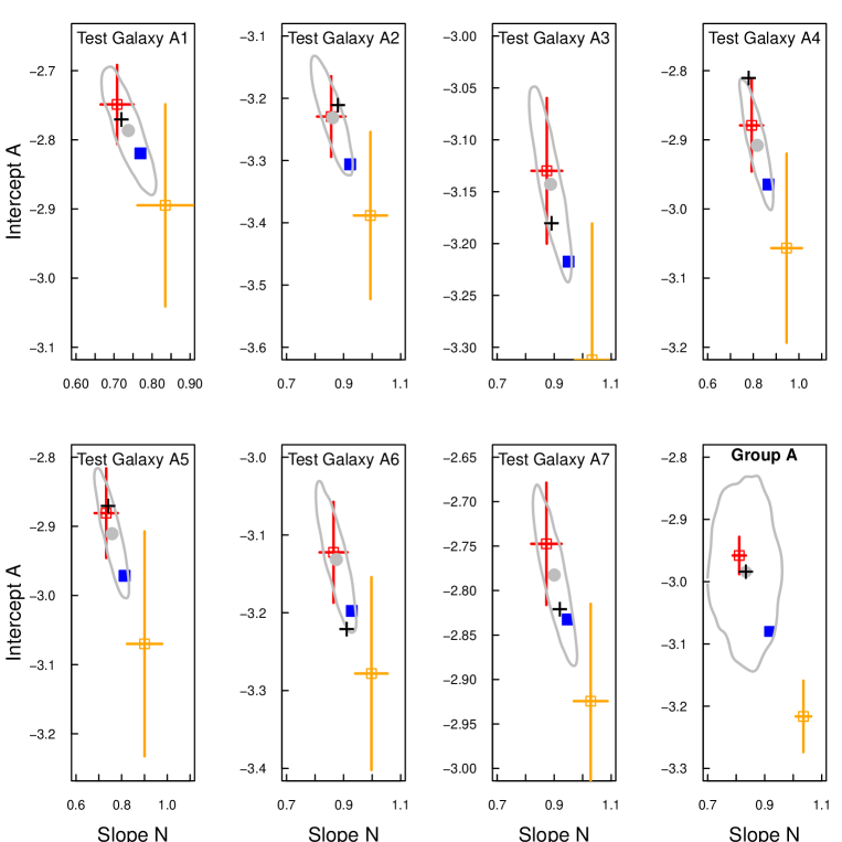
Figure 1: Slope and intercept of test galaxies in Group A. Black cross shows the true values. Red and orange squares show the OLS$(\Sigma_{\rm SFR}|\Sigma_{\rm mol})$ and OLS$(\Sigma_{\rm mol}|\Sigma_{\rm SFR})$ results, with their $1\sigma$ uncertainties, respectively. The gray circles indicate the estimate provided by the median of hierarchical Bayesian posterior result, and the contours mark the $1\sigma$ deviation. The filled blue squares mark the bisector estimates. The last panel on the bottom row shows the group parameters and fit estimates.

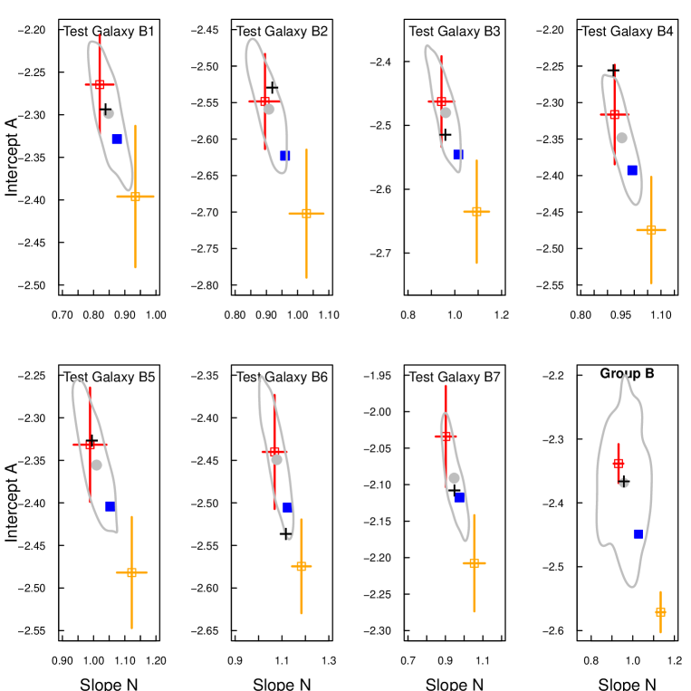
Figure 2: Slope and intercept, along with parameter estimates, of test galaxies in Group B. Symbols and contours are defined in the same fashion as in Figure 1.

3.2 Comparison with ordinary least squares methods

In order to assess how the hierarchical Bayesian modelling compares to other fitting methods, we perform three OLS fits: the $y|x$, $x|y$, hereafter OLS$(\Sigma_{\rm SFR}|\Sigma_{\rm mol})$, and OLS$(\Sigma_{\rm mol}|\Sigma_{\rm SFR})$, respectively, and an OLS bisector (e.g. Isobe et al., 1990). The estimated slope of the OLS fits is dependent on the covariance of the data, and variance of the quantity labeled as the predictor or what is considered the independent quantity, as further discussed below. In order not to place a preference on $\Sigma_{\rm SFR}$ or $\Sigma_{\rm mol}$, the bisector fit has emerged as the preferred method in fitting KS relationships.

The estimates from these three OLS fitting methods, however, should not be interpreted as the same quantities, as discussed by Isobe et al. (1990, see also Gelman & Hill 2007). An OLS($y|x$) estimates the conditional mean of “y given x”. Accordingly, as the constructed relationships, or simulations, describe how the mean value of log($\Sigma_{\rm SFR}$) depends on log($\Sigma_{\rm mol}$), the OLS$(\Sigma_{\rm SFR}|\Sigma_{\rm mol})$ is the most applicable. The OLS$(\Sigma_{\rm mol}|\Sigma_{\rm SFR})$ estimates how the mean value of log($\Sigma_{\rm mol}$) depends on log($\Sigma_{\rm SFR}$), and the bisector estimates are weighted means between the OLS$(\Sigma_{\rm mol}|\Sigma_{\rm SFR})$ and OLS$(\Sigma_{\rm SFR}|\Sigma_{\rm mol})$ - the details of the slope estimates of the different OLS fits are provided below. The three OLS results will provide different estimates, as they are different statistics derived from the joint distribution of the measurements. The choice of which quantity should be identified as the “x” or “y” variable should be motivated by the scientific goals. For the KS law, we are primarily interested in how $\Sigma_{\rm SFR}$ varies with $\Sigma_{\rm mol}$. As a result, we would expect the OLS$(\Sigma_{\rm SFR}|\Sigma_{\rm mol})$ to provide more accurate estimates of the underlying parameters of the simulation for a single galaxy, in the absence of noise. Yet, the simulation includes noise and intrinsic scatter, important properties that a simple OLS$(\Sigma_{\rm SFR}|\Sigma_{\rm mol})$ does not account for. As the bisector fit has been employed to estimate the KS parameters in previous works, we also compare those estimates to the Bayesian result. Following conventional practice, for estimating the group parameters we simply apply the fit to all data from the seven galaxies together.

Tables 3 and 4 provide the results of the fits. We show the $2\sigma$ uncertainties along with the OLS best fit parameters. These best fit values, along with the $1\sigma$ uncertainties for the OLS$(\Sigma_{\rm SFR}|\Sigma_{\rm mol})$ and OLS$(\Sigma_{\rm mol}|\Sigma_{\rm SFR})$ estimates, are also shown in Figures 1 and 2.

Tables 3 and 4, as well as Figures 1 and 2, indicate that the bisector consistently overestimates the slopes (and underestimates the intercepts), for all individuals within the groups, as well as the group estimate. The results of the OLS$(\Sigma_{\rm SFR}|\Sigma_{\rm mol})$ and OLS$(\Sigma_{\rm mol}|\Sigma_{\rm SFR})$ are rather discrepant, leading to a bisector parameter estimate falling between those results.

That the estimates from the OLS fitting vary between the three different methods, as well in comparison to the Bayesian estimates, can be understood by the definition of the slopes and intercepts in least-squares fitting. The OLS parameters have been extensively discussed and presented (e.g. Isobe et al., 1990; Kelly, 2007), so we simply state the slope definitions here. For an OLS$(\Sigma_{\rm SFR}|\Sigma_{\rm mol})$ fit, the slope $N_{\Sigma_{\rm SFR}|\Sigma_{\rm mol}}$ is computed by taking the ratio of the covariance (Cov) between the data and the variance (Var) in the predictor $\Sigma_{\rm mol}$:

$$N_{\Sigma_{\rm SFR}|\Sigma_{\rm mol}}=\frac{{\rm Cov}({\hat{\Sigma}_{\rm mol}},{\hat{\Sigma}_{\rm SFR})}}{{\rm Var}({\hat{\Sigma}_{\rm mol}})}$$ (29)

For the OLS$(\Sigma_{\rm mol}|\Sigma_{\rm SFR})$, the fit slope is the inverse of the desired quantity in Equation 2, so that:

$$N_{\Sigma_{\rm mol}|\Sigma_{\rm SFR}}=\frac{{\rm Var}({\hat{\Sigma}_{\rm SFR})}}{{\rm Cov}({\hat{\Sigma}_{\rm mol}},{\hat{\Sigma}_{\rm SFR}})}$$ (30)

The bisector slope $N_{\rm Bis}$ is a weighted mean of the OLS$(\Sigma_{\rm SFR}|\Sigma_{\rm mol})$ and OLS$(\Sigma_{\rm mol}|\Sigma_{\rm SFR})$ slopes.

$$N_{\rm Bis}=(N_{\Sigma_{\rm mol}|\Sigma_{\rm SFR}}+N_{\Sigma_{\rm SFR}|\Sigma_{\rm mol}})^{-1}$$ (31)

$$\times\biggl{[}N_{\Sigma_{\rm SFR}|\Sigma_{\rm mol}}N_{\Sigma_{\rm mol}|\Sigma_{\rm SFR}}-1+$$

$$\sqrt{(1+N^{2}_{\Sigma_{\rm SFR}|\Sigma_{\rm mol}})(1+N^{2}_{\Sigma_{\rm mol}|\Sigma_{\rm SFR}})}\biggl{]}$$

Equations 29 - 31 illustrate what we stated earlier: that the three different slope estimates are just three different statistics (or summaries) derived from the same joint distribution. Choosing one estimate over the other does not imply that one quantity “causes” the other, as is sometimes claimed to be implied by the terminology of “independent” and “dependent” variables. However, the different slope estimates do differ in interpretation. The OLS$(\Sigma_{\rm SFR}|\Sigma_{\rm mol})$ slope describes how the mean value of $\Sigma_{\rm SFR}$ varies with $\Sigma_{\rm mol}$  while the OLS$(\Sigma_{\rm mol}|\Sigma_{\rm SFR})$ slope describes how the mean value of $\Sigma_{\rm mol}$ changes with $\Sigma_{\rm SFR}$. Thus, both OLS slopes are easily interpretable. In contrast, the bisector slope is a weighted average of the two OLS slope, and it is not clear how this should be interpreted.

The OLS slopes are therefore strongly dependent on the statistical properties of ${\hat{\Sigma}_{\rm SFR}}$ and ${\hat{\Sigma}_{\rm mol}}$. For the synthetic data of both groups, Var(${\hat{\Sigma}_{\rm mol}}$) = 0.39, pooling all data from each galaxy together. For Group A, Var(${\hat{\Sigma}_{\rm SFR}}$) = 0.33, and Cov(${\hat{\Sigma}_{\rm mol}}$, ${\hat{\Sigma}_{\rm SFR}}$) = 0.32. In Group B, Var(${\hat{\Sigma}_{\rm SFR}}$) = 0.41, and Cov(${\hat{\Sigma}_{\rm mol}}$, ${\hat{\Sigma}_{\rm SFR}}$) = 0.36. The covariances and Var(${\hat{\Sigma}_{\rm SFR}}$) of the two groups are similar, as the adopted slopes only differ by $\approx$ 10%. More importantly, the covariance is $<$ 1. As the covariance occurs in the denominator of the OLS$(\Sigma_{\rm mol}|\Sigma_{\rm SFR})$ slope, but in the numerator of the OLS$(\Sigma_{\rm SFR}|\Sigma_{\rm mol})$ slope (and the variances of the chosen predictors are similar), the resulting $N_{\Sigma_{\rm mol}|\Sigma_{\rm SFR}}>N_{\Sigma_{\rm SFR}|\Sigma_{\rm mol}}$.

Notice that the OLS$(\Sigma_{\rm SFR}|\Sigma_{\rm mol})$ parameter estimates are closer to the true value than the OLS$(\Sigma_{\rm mol}|\Sigma_{\rm SFR})$ estimates. This is to be expected, because as described above the OLS$(\Sigma_{\rm SFR}|\Sigma_{\rm mol})$ estimates how the mean value of log($\Sigma_{\rm SFR}$) depends on log($\Sigma_{\rm mol}$), and the simulated datasets are constructed with a linear relation between those quantities. For these data, the Cov(${\hat{\Sigma}_{\rm mol}}$, ${\hat{\Sigma}_{\rm SFR}}$) is less than the variance of either quantity, thereby leading to $N_{\Sigma_{\rm SFR}|\Sigma_{\rm mol}}<1$ and $N_{\Sigma_{\rm mol}|\Sigma_{\rm SFR}}>1$. The OLS$(\Sigma_{\rm mol}|\Sigma_{\rm SFR})$ result therefore drives the bisector slope towards larger values, leading to the systematic overestimates shown in Tables 3-4 and Figures 1-2. The overestimate in the bisector slope is not as drastic for Test Group B, because the underlying slopes are closer to unity to begin with. Further, note that tests performed by Isobe et al. (1990) (see their Table 2) produce bisector slopes of unity for a number of scenarios, where the $y|x$ or $x|y$ slopes are far from unity. In fact, the bisector fit is expected to produce a slope of one when $x$ and $y$ are statistically independent, indicative of the difficulty in interpreting the bisector. If the scatter about a linear relationship were very low, for instance due to small measurement uncertainties, then the OLS$(\Sigma_{\rm SFR}|\Sigma_{\rm mol})$ and OLS$(\Sigma_{\rm mol}|\Sigma_{\rm SFR})$, and correspondingly the bisector, would accurately recover the regression parameters. Taken together, one can assess the accuracy of the bisector estimated regression parameters by inspecting both the OLS$(y|x)$ and OLS$(x|y)$ results. If they are highly discrepant, then the bisector result, which will fall between the OLS$(y|x)$ and OLS$(x|y)$ estimates, should not be considered to provide accurate parameter estimates of a linear relationship.

3.3 Effect of Model Assumptions

For the two synthetic datasets considered so far, the normal distributions in the intrinsic scatter and measurement uncertainties matches the prior distributions in the hierarchical model. In order to test the sensitivity of these assumptions, we consider an another synthetic dataset with uniform distributions for the uncertainty and scatter. Additionally, compared with the previous tests the synthetic dataset we consider here has more individual galaxies, with different numbers of (${\hat{\Sigma}_{\rm mol}}$, ${\hat{\Sigma}_{\rm SFR}}$) pairs for each individual.

The intrinsic slopes and intercepts of each synthetic galaxy in Test Group C varies between 0.7 to 1.5 and $-$3.0 to $-$2.0, respectively. The population mean value of the slope is 1.1, and the mean intercept is $-$2.5. The intrisic scatter term is uniformly distributed centered on 0, with extent 0.3. To construct the noisy measurements ${\hat{\Sigma}_{\rm mol}}$ and ${\hat{\Sigma}_{\rm SFR}}$, we add a random value drawn from a uniform distribution centered about 0, with extents 0.2 and 0.25, respectively. We carry out the Bayesian fit as before, where we assume Gaussian distributions, with $1\sigma$ noise estimates equal to the width of the uniform distributions employed to construct the noisy datasets. We also compare the Bayesian results with the direct OLS fits.

Table 5 shows the intrinsic and Bayesian estimated parameters. For the slope and intercept parameter estimates of the individuals, the true values are always contained within the $2\sigma$ interval, except for the slope of Test Galaxy C1 and intercept of Test Galaxy C2, which have the fewest number of datapoints. Further, for these individuals the intrinsic parameters are far from the mean value, so the Bayesian estimates are affected by shrinkage, which was described above. Notice that the group parameter estimates also recover the intrinsic values, and that the posterior median is close to the true values.

The OLS fit results for the population in Table 6 show a marked difference compared to the Bayesian estimates. Even at the $2\sigma$ level, neither the OLS$(\Sigma_{\rm SFR}|\Sigma_{\rm mol})$ and OLS$(\Sigma_{\rm mol}|\Sigma_{\rm SFR})$ can recover the true value. Consequently, the bisector estimates are also discrepant from the intrinsic parameters. For the OLS group estimates, all datapoints are fit simultaneously, so those individuals with the largest number of datapoints dominate the final fit. Therefore, the OLS parameter estimates tend towards smaller slopes and larger intercepts, thereby underestimating the group slope and overestimating the intercept, even when considering the full $2\sigma$ interval. This discrepancy, especially for the OLS$(\Sigma_{\rm SFR}|\Sigma_{\rm mol})$ case, is larger than that from Test Groups A and B, due to the variable number of datapoints between individuals, as well as the higher noise and scatter levels.

This test has shown that the Bayesian posterior can reasonably recover the slopes and intercepts of the individual even though the assumed distributions for the noise and scatter terms are incorrect. The $2\sigma$ ranges of the posterior only provide erroneous subject estimates when the individual has very few datapoints, and/or the individual parameters are far from the population mean values. Nevertheless, the population values are recovered, indicating a marked improvement of the Bayesian result compared to the OLS fits.

Notice that the Bayesian estimate of the scatter is systematically lower than the intrinsic value. This occurs because the chosen $1\sigma$ value for the noise is set to the extent of the true uniform noise distribution. Accordingly, in the synthetic data there are no measured datapoints occuring at greater than $1\sigma$ from the true values, whereas the Bayesian model assumes that such noisy measurment do exist. Due to this overestimate of the noise properties, the Bayesian model erroneously designates some of the intrinsic scatter to be associated with noise uncertainty, and thereby underestimates the intrinsic scatter.

Clearly, the accuracy of the Bayesian fits are dependent on the assumed distributions. If there is good correspondence between the assumed and intrinsic distributions, as in Test Groups A and B, the Bayesian results will be highly accurate. If there is large discrepancy in the assumed and intrinsic distribution, then the accuracy Bayesian result will be degraded, as for Test Group C. Nevertheless, we have shown that for uniformly distributed noise and scatter properties, the hierarchical Bayesian method employing normal priors for these properties can nevertheless accurately recover the population parameters, especially when compared with the OLS methods. The magnitude of the discrepancy is of course dependent on the noise and scatter properties. Further tests may be needed for ascertaining the reliability of the model on datasets with more discrepant distributions. When interpreting the results from the application of the method to observed datasets, one must of course bear in mind that the accuracy is dependent on the priors. As we have considered two tests in Section 3.2 that we consider to be representative of real observations, we have confidence that the hierarchical model is appropriate for the observed datasets we analyze in Section 5.

3.4 Summary of method testing

We have tested the hierarchical Bayesian model described in Section 2 using three sets of synthetic data. The datasets consists of groups containing numerous individual galaxies. Each galaxy is characterized by some chosen power-law relationship between $\Sigma_{\rm SFR}$ and $\Sigma_{\rm mol}$, as well as intrinsic scatter about this relationship. We include noise, similar to estimated uncertainties from the observations, to produce ${\hat{\Sigma}_{\rm SFR}}$ and ${\hat{\Sigma}_{\rm mol}}$. The hierarchical Bayesian method can accurately recover the underlying parameter estimates, as the peaks of the posterior are very close to the true values for each individual as well as the mean population parameters, and the whole $2\sigma$ range includes the correct solution.

The synthetic datasets do not strictly satisfy all aspects of the priors in the hierarchical model. Namely, for Test Groups A and B, the slope and intercepts of the seven individual galaxies are not drawn from a normal distribution for the group. Similarly, the gas surface densities of each galaxy are not normally distributed, but rather uniformly distributed. That the method is able to accurately recover the underlying slopes and intercepts indicates the insensitivity of the parameter estimates to these priors. With Test Group C, we examine the situation where the intrinsic and noise distributions are uniformly distributed, which is discrepant from the assumption of Gaussian distributions in the hierarchical model. This group has twenty individuals, each containing a different number of datapoints. For this test, the Bayesian fit again accurately recovers the population slopes and intercepts. The $2\sigma$ range of the posterior only misses the slope and intercept for the individuals that have the fewest datapoints and the most discrepant slope and intercept relative to the population values.

The Bayesian fit proves to be more accurate than the OLS fits, especially compared to the often employed bisector fit. As discussed, however, the bisector is expected to estimate a slope which falls between OLS$(\Sigma_{\rm SFR}|\Sigma_{\rm mol})$ and OLS$(\Sigma_{\rm mol}|\Sigma_{\rm SFR})$ slopes, and is therefore difficult to interpret. The bisector should not be considered to provide an estimate of $N$ in Equation 2. The hierarchical Bayesian result does provide an estimate of this quantity, and its results are easily interpretable: we can estimate the mean value of $\Sigma_{\rm SFR}$ given $\Sigma_{\rm mol}$, for each individual galaxy as well as for the population.

4 Observations

We are now in a position to apply the Bayesian method on observational datasets. For its first application, the dataset consists of a sample of seven spiral galaxies from B08, and is publicly available in Bigiel et al. (2010). For six of the galaxies, ${\hat{\Sigma}_{\rm mol}}$ is measured in 750 pc-sized regions from the ¹²CO $J=2-1$ observations in the HERACLES survey (Leroy et al., 2009). For the remaining galaxy, M51, ${\hat{\Sigma}_{\rm mol}}$ is computed from ¹²CO $J=1-0$ observations from the BIMA SONG survey (Helfer et al., 2003). The CO intensities are converted to gas surface densities using a constant $X_{\rm CO}$ factor, and a constant ¹²CO ($J=2-1)/(J=1-0)$ ratio (see B08 and Bigiel et al. 2010 for details) . We explore variations in $X_{\rm CO}$ in Section 5.2. To estimate ${\hat{\Sigma}_{\rm SFR}}$, B08 use the combination of 24 µm intensities from the SINGS survey (Kennicutt et al., 2003), and UV fluxes from the GALEX survey (Gil de Paz et al., 2007). We refer the reader to B08 and Leroy et al. (2008, 2009) for details of these observations.

5 Results

5.1 Application to B08 Data

The results of the hierarchical Bayesian fit on the seven spiral galaxies from B08 are shown in Table 7. The median value of the slopes are all lower than unity, and for four of the galaxies, NGC 5194 (M51), NGC 5055, NGC 6946, and NGC 628, a linear slope can be excluded at $>95\%$. The median of the inferred group slope is 0.84, with unity falling just inside the $2\sigma$ interval.

Table 7: Bayesian estimated parameters for the seven spiral galaxies in B08

Subject	Bayes $A$	Bayes $2\sigma_{A}$	Bayes $N$	Bayes $2\sigma_{N}$	Bayes $\sigma_{\rm scat}$
NGC 5194 (M51)	$-$2.84	[$-$3.0, $-$2.7]	0.72	[0.62, 0.83]	0.06
NGC 5055	$-$3.20	[$-$3.3, $-$3.1]	0.87	[0.79, 0.95]	0.04
NGC 3521	$-$3.20	[$-$3.4, $-$3.0]	0.90	[0.76, 1.03]	0.05
NGC 6946	$-$2.81	[$-$2.9, $-$2.7]	0.78	[0.70, 0.86]	0.11
NGC 628	$-$2.89	[$-$3.1, $-$2.6]	0.76	[0.51, 0.95]	0.05
NGC 3184	$-$3.24	[$-$3.4, $-$3.1]	0.92	[0.79, 1.10]	0.05
NGC 4736	$-$2.83	[$-$3.2, $-$2.4]	0.92	[0.67, 1.20]	0.08
Group Parameters	$-$3.00	[$-$3.3, $-$2.7]	0.84	[0.63, 1.0]	0.14

We can verify that the model can reasonably reproduce the data by over-plotting representative regression lines constructed from the posterior parameters estimates. From the posterior PDF, we can draw a large number of $A$, $N$, and $\sigma_{\rm scat}$ values, and evaluate Equation 2 at various $\Sigma_{\rm mol}$ (for each galaxy). Figure 3 shows the data and 50 random draws from the posterior (gray lines) for each galaxy, demonstrating that the Bayesian model is consistent with the data. For comparison, the red dashed line shows the linear relationship inferred from a bisector fit on all data. The last panel in Figure 3 only shows the data from all the galaxies and the associated bisector result. As this ensemble is not directly used to infer the group parameters, we do not overlay the inferred group lines.

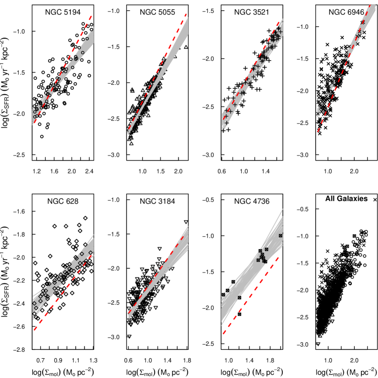
Figure 3: Hierarchical Bayesian fits (gray lines), along with the data (black symbols), from the B08 sample of seven galaxies (see Fig. 4 in B08). Gray lines show 50 random draws from the posterior. For reference, (red) dashed lines show the same linear relationship from a bisector fit to all data in the last panel. Note that the axes are different in each panel.

The Bayesian inferred parameters are rather different from the parameters inferred from the bisector fit. The bisector results are adopted as the true values of our synthetic dataset in Group B, and are shown in Table 2 in Section 3. Recall that the hierarchical Bayesian fit on that Group accurately recovered the model parameters, as shown in Figure 2 and Table 2. However, the bisector fit produces slope estimates which are larger than the model slope, and underestimated the intercept, similar to the results from Group A. In Group A, the results of the Bayesian fit from the observed data (Table 2) were adopted as the parameters. For that test group, the Bayesian result again accurately recovered the adopted parameters. Recall that the bisector slope is a weighted mean of the OLS$(\Sigma_{\rm SFR}|\Sigma_{\rm mol})$ and OLS$(\Sigma_{\rm mol}|\Sigma_{\rm SFR})$ estimates. For the ensemble B08 data, the OLS$(\Sigma_{\rm SFR}|\Sigma_{\rm mol})$ and OLS$(\Sigma_{\rm mol}|\Sigma_{\rm SFR})$ slopes (and $2\sigma$ uncertainty) are 0.84$\pm$0.04 and 1.19$\pm$0.04, respectively. As discussed in Section 3.2, the large discrepancy between the OLS slope estimates is a clear indicator that measurement uncertainties in $\Sigma_{\rm SFR}$ and $\Sigma_{\rm mol}$ are affecting the OLS estimates.

The observed and synthetic data also differ in the detailed statistics of ${\hat{\Sigma}_{\rm SFR}}$ and ${\hat{\Sigma}_{\rm mol}}$. For all data pooled together, Var(${\hat{\Sigma}_{\rm mol}}$) = 0.15, Var(${\hat{\Sigma}_{\rm SFR}}$) = 0.15, and Cov(${\hat{\Sigma}_{\rm mol}}$, ${\hat{\Sigma}_{\rm SFR}}$) = 0.12. These values are a factor of 2$-$3 lower than the statistics of the synthetic data discussed in Section 3.2. This indicates that there are some differences between the synthetic dataset we considered, and the observed data. Much of the difference can be attributed to ${\hat{\Sigma}_{\rm mol}}$. For the synthetic datasets in Section 3, we simply considered a uniform distribution in $\Sigma_{\rm mol}$, whereas the measured $\Sigma_{\rm mol}$ in each galaxy is not necessarily uniformly distributed. Nevertheless, the tests in Section 3 showed that the Bayesian parameter estimates are not sensitive to the intrinsic $\Sigma_{\rm mol}$ distribution. Further, note that the $\sigma_{\rm scat}$ estimates in Table 7 are all  $\buildrel<\over{\sim}$ 0.1. This suggests that a power law relationship can reasonably describe the observed trends. Taken together with the results of the tests, any discrepancy in the true and prior distributions of $\Sigma_{\rm mol}$ and $\sigma_{\rm scat}$ likely does not strongly effect the parameter estimates.

However, the assumed values of the conversion factors may play a stronger role in the determination of the KS parameters. We have considered ${\hat{\Sigma}_{\rm mol}}$ and ${\hat{\Sigma}_{\rm SFR}}$ directly, such that there is no uncertainty in the conversion from luminosities to those quantities. Here, we have assumed $X_{\rm CO}$ to be fixed at 2$\times 10^{20}$ cm^-2 K^-1 km^-1 s, but in the next subsection we explore variations in $X_{\rm CO}$ under the hierarchical Bayesian framework.

We can also compare the Bayesian result to the OLS$(\Sigma_{\rm SFR}|\Sigma_{\rm mol})$ and OLS$(\Sigma_{\rm mol}|\Sigma_{\rm SFR})$ estimates. As described in Section 3.2, the OLS$(\Sigma_{\rm SFR}|\Sigma_{\rm mol})$ should produce the most accurate estimates, because by definition it estimates the mean value of $\Sigma_{\rm SFR}$ given $\Sigma_{\rm mol}$. To evaluate the OLS slopes, we only need to consider the covariances and variances of the data. The ratio of Cov(${\hat{\Sigma}_{\rm mol}}$, ${\hat{\Sigma}_{\rm SFR}}$)/Var(${\hat{\Sigma}_{\rm mol}}$) is 0.8, equivalent to the ratio of the ensemble in Group A, and by definition to the OLS$(\Sigma_{\rm SFR}|\Sigma_{\rm mol})$ fit slope of both the observed sample and the synthetic data in Group A. The OLS$(\Sigma_{\rm SFR}|\Sigma_{\rm mol})$ slope is similar to the Bayesian result, though the estimated uncertainty is very small, 0.04. This uncertainty is solely statistical, does not account for measurement errors, and its low value is primarily driven by the large number of datapoints (981). Consequently, the OLS methods significantly underestimate the errors, and they do not provide the parameter estimates of the individuals galaxies when all data are fit simultaneously. We therefore caution against the use of such statistical uncertainties for characterizing the quality of the linear regression on large datasets.

To assess the difference between the hierarchical modeling and the parameter estimates inferred from all data, we perform a direct Bayesian fit to the ensemble. For this analysis, we do not require a group level in the hierarchical model. In this case, we are only interesting in estimating $N$, $A$, and the scatter term $\sigma_{\rm scat}$ for the ensemble, shown in the last panel of Figure 3. We thus simplify the hierarchical model described in Section 2.4 by eliminating the group level, and employ uninformed priors on the slope, intercept, and scatter terms. We treat measurement uncertainties in the same manner as described in Section 2.4. The posterior median of the Bayesian regression analysis of the combined data yields $N$=0.90, with $2\sigma$ range [0.88, 0.95]. This result is substantially different from the parameter estimates from the full hierarchical model, and would lead to different conclusions regarding the KS relationship. Namely, though the inferred slope is still less than unity, the slope estimates for two of the individual galaxies, M51 and NGC 6946, are excluded at the 95% level. Related to that discrepancy, the limited range in the $2\sigma$ estimated slope of the ensemble suggests that there may be a “universal” KS index. However, the full hierarchical Bayesian result provides a larger range for the estimated group parameters and unambiguous differences between individual galaxy parameters. That indicates that there is likely no universal KS relationship which can accurately describe the $\Sigma_{\rm SFR}$- $\Sigma_{\rm mol}$ relationship for all galaxies, if our assumptions about the conversion factors are valid, as further discussed in the next section. The variations in KS relationships between galaxies is clearly apparent simply by inspecting the datapoints in Figure 3, affirming the variable star formation behaviour in different galaxies identified by the hierarchical Bayesian fit.

5.2 Variations in the $X_{\rm CO}$ factor

In the analysis thus far, we have assumed that the conversion from observed intensities to the star formation rates and molecular gas surface densities are exact. We thus implicitly assume that $\Sigma_{\rm SFR}$ and $\Sigma_{\rm mol}$ are directly measured. But in actuality, the observed quantities are UV, 24 µm, and CO intensities, which are converted to star formation rates and gas surface densities using constant conversion factors. Uncertainties in the conversion factors have thus not been considered in the regression analysis.

A major advantage of the hierarchical framework is that uncertainties in any quantity can be easily incorporated - for instance by including additional levels for the conversion factors. By explicitly implementing another level for the conversion factors, the hierarchical analysis can probabilistically ascertain whether certain values of the conversion factors drive tighter KS relationships. Here, we demonstrate the capability of the method to treat uncertainties in the $X_{\rm CO}$, allowing for independent variations in $X_{\rm CO}$ between each datapoint. In this framework, we are simply considering statistical variations in $X_{\rm CO}$. As we describe below, observational and theoretical efforts may further constrain this conversion factor.

In using the observed CO intensity $\hat{I}_{\rm CO}$ rather than ${\hat{\Sigma}_{\rm mol}}$, we assume a measurement uncertainty similar to that described in Section 2.3. Accordingly, we consider a linear regression of the form:

$$\log(\Sigma_{\rm SFR})=A+N\log(X_{\rm CO}I_{\rm CO})+\epsilon_{\rm scat}$$ (32)

In this case, we need another level for the distribution of $X_{\rm CO}$:

$$X_{\rm CO}\sim\mathcal{U}({\rm min}X_{\rm CO},{\rm max}X_{\rm CO}),$$ (33)

where $\mathcal{U}$ is a uniform distribution between min$X_{\rm CO}$ and max$X_{\rm CO}$. We have explored different extents for the ranges in $X_{\rm CO}$, including up to an order of magnitude, and find insignificant differences in the results, either on the individual or group level. The $2\sigma$ ranges increases slightly, but the mean/median of the posterior does not change. This indicates that independent variations in $X_{\rm CO}$ do not have a strong influence on the KS parameters for this sample.

As an example, Table 8 shows the individual and group slopes and scatter terms from the sample where $X_{\rm CO}$ is allowed to vary from min$X_{\rm CO}$=0.5$\times 10^{20}$ and max$X_{\rm CO}$=8$\times 10^{20}$ cm^-2 K^-1 km^-1 s, allowing for over an order of magnitude variation in $X_{\rm CO}$. The median of the group slope is 0.79, and the $2\sigma$ interval is 0.58 to 1.0, which is slightly larger than the range shown in Table 7. There are hardly any differences between these results and the parameter estimates when $X_{\rm CO}$ is fixed. One difference is that the slopes are systematically lower by  $\buildrel<\over{\sim}$ 0.1. Yet, there is significant overlap between the results, considering the full 95% intervals, so there is no strong evidence of a decrease in slopes. Further, the $\sigma_{\rm scat}$ values are similar between the two fits, again suggestive that varying $X_{\rm CO}$ (by about an order of magnitude) does not produce tighter KS relationships. Similarly, the hierarchical Bayesian fit does not provide any evidence for a preferred value of $X_{\rm CO}$.

Table 8: Bayesian estimated slopes and scatter for the seven spiral galaxies in B08, where the $X_{\rm CO}$ factor is allowed to vary from 0.5$\times 10^{20}$ to 8$\times 10^{20}$ cm^-2 K^-1 km^-1 s

Subject	Bayes $N$	Bayes $2\sigma_{N}$	Bayes $\sigma_{\rm scat}$
NGC 5194 (M51)	0.67	[0.57, 0.78]	0.07
NGC 5055	0.86	[0.78, 0.94]	0.04
NGC 3521	0.88	[0.76, 1.02]	0.05
NGC 6946	0.74	[0.66, 0.81]	0.13
NGC 628	0.65	[0.45, 0.85]	0.05
NGC 3184	0.84	[0.72, 0.97]	0.05
NGC 4736	0.86	[0.59, 1.10]	0.09
Group Parameters	0.79	[0.58, 1.0]	0.14

For this initial investigation into the effect of uncertainty in the conversion factor, we assume that $X_{\rm CO}$ does not correlate with any other property. This preliminary analysis has only allowed for a modest variation in $X_{\rm CO}$, with no constraint for each datapoint beyond the range set by conditional relationship (33). Recent theoretical efforts have indicated that $X_{\rm CO}$ indeed varies with other physical properties, such as metallicity (Glover & Mac Low, 2011; Shetty et al., 2011a), gas temperature, velocity dispersion (Narayanan et al., 2011; Shetty et al., 2011b) or with molecular gas content (Feldmann et al., 2012b; Narayanan et al., 2012). Observational investigations are also finding evidence for variable $X_{\rm CO}$ in individual galaxies (e.g. Sandstrom et al., 2012). Such systematic variations would result in different KS parameters (see, e.g. Ostriker & Shetty, 2011; Narayanan et al., 2012). We will investigate how the KS relationship is affected by these systematic variations in $X_{\rm CO}$ in future work. To improve the parameter estimates, it would be helpful to increase the number of sample galaxies and to incorporate uncertainties in converting IR and UV luminosities to $\Sigma_{\rm SFR}$. We can further explore other parametrizations in $X_{\rm CO}$, e.g. as a function of $I_{\rm CO}$, and either for individual galaxies or for the population. Such modelling will allow for a study into the correlation between the parameters, e.g. $X_{\rm CO}$ with $\Sigma_{\rm mol}$, in addition to fully treating measurement and conversion factor uncertainties.

6 Discussion & Summary

6.1 Advantages of hierarchical Bayesian modelling

We have demonstrated that the Bayesian method described in Section 2 can accurately recover the regression parameters from a sample containing hierarchical structure. Hierarchical data refers to any set with numerous measurements from individuals within a group (e.g. measurements from a sample of galaxies, with a number of measurements per galaxy). The method self-consistently treats measurement uncertainties, so that the resulting parameter estimates are PDFs which account for any uncertainty in the modelling process.

The Bayesian method is shown to be superior to the commonly employed OLS estimates that usually do not consider the hierarchical structure in the dataset. Besides accounting for the measurement uncertainties, the hierarchical nature of the dataset is preserved, as the Bayesian method simultaneously estimates the parameters of both the individuals as well as the population. Under this framework, differences between individuals are clearly exposed, and the range in plausible group parameters self-consistently permits for variations between individuals.

Another key aspect of the hierarchical Bayesian method is the robust estimation of the scatter $\sigma_{\rm scat}$ about the fit regression line, for both individuals subjects as well as the group. When assessing the KS relationship from observations, there is a trend of decreasing $\sigma_{\rm scat}$ with increasing aperture size (e.g. Thilker et al., 2007; Kennicutt et al., 2007; Rahman et al., 2011). Theoretical efforts have considered $\sigma_{\rm scat}$ and its relationship to sampling size. It may be due to variable sampling of the underlying cloud mass spectrum (Calzetti et al., 2012), influence on averaging timescale, metallicity (Dib, 2011), background radiation field (Feldmann et al., 2011), or simply transient effects (e.g. Shetty & Ostriker, 2008). With credible knowledge of the measurement uncertainties (e.g. $\sigma_{\rm mol}$ and $\sigma_{\rm SFR}$), the Bayesian method will provide accurate estimates of the intrinsic scatter in the KS relationship. Future work considering the possibility of variable conversion factors for deriving $\Sigma_{\rm SFR}$ and $\Sigma_{\rm mol}$ will provide even more accurate estimates of the intrinsic scatter, as the scatter due to the systematics can be robustly separated from the intrinsic scatter. These estimates of the intrinsic scatter can thereafter be used for quantitative comparisons with theoretical results.

Recently, new statistical methods have been considered beyond the bisector to estimate the KS parameters. Namely, Blanc et al. (2009) create numerous $\Sigma_{\rm SFR}$$-$$\Sigma_{\rm mol}$ grids, considering different model KS parameters, a scatter term, and different realizations of noise. Then, they assess the $\chi^{2}$ between all the model grids and that produced from observations of M51. The distribution of $\chi^{2}$ values identifies the best-fit parameters and their uncertainties. As this Monte Carlo approach considers the scatter term as well as treats uncertainties, it should be more accurate than the typical OLS bisector. It has also recently been utilized in Leroy et al. (2012, Submitted) on the HERACLES sample. It will be interesting to ascertain whether such a method can accurately recover the individual and group parameters from a sample of galaxies, and how it compares to the hierarchical Bayesian method presented here.

6.2 The KS relationship in galaxies

As discussed in the introduction, the KS law is a widely investigated relationship between the star formation rate and molecular gas surface density. The initial works using galaxy wide averages estimated N$\approx$1.5. Follow up work using background subtracted emission from resolved observations by Kennicutt et al. (2007) and Liu et al. (2011) recovered this result. On the other hand, kpc-scale observations of a large sample of galaxies have inferred slopes closer to unity (e.g. B08, Bigiel et al. 2011; Leroy et al. 2008, Leroy et al. 2012 Submitted, Rahman et al. 2012).

After verifying the accuracy of the hierarchical Bayesian method, which models how the mean value of log($\Sigma_{\rm SFR}$) depends on log($\Sigma_{\rm mol}$), we applied the method to estimate the parameters of the KS relationship in the sample of disk galaxies from B08. The fitting results from both the test samples (Section 3) and the B08 sample suggest that previous methods have overestimated the KS slopes. The hierarchical Bayesian method produces slopes which are slightly lower than unity, especially when considering the full 95% confidence interval for some of the individual galaxies.

Before interpreting our results from this analysis, we note a number of important caveats which should be kept in mind. First, as we have discussed throughout this work, we have directly considered ${\hat{\Sigma}_{\rm SFR}}$ and ${\hat{\Sigma}_{\rm mol}}$. Yet, these are not directly measured. The star formation rates and surface densities are estimated from the observables (e.g., CO, UV and IR intensities) using constant conversion factors. In the measurement model (Eqns. 4-5), we have only accounted for random statistical errors associated with observational noise. Yet, systematic errors may arise in the conversion between intensities to ${\hat{\Sigma}_{\rm SFR}}$ and ${\hat{\Sigma}_{\rm mol}}$. Under a hierarchical framework, uncertainties in these conversion factors can be naturally handled, including correlated errors between the various coefficients. In future work, we will self-consistently treat the uncertainties in these conversion factors for a larger sample of galaxies. This may reveal interesting new aspects of the star formation and gas properties in the ISM.

Additionally, we have not considered the different approaches to estimating star formation rates on $\sim$kpc scales in galaxies. As Kennicutt et al. (2007), Liu et al. (2011), and Rahman et al. (2011) demonstrate, subtracting off a diffuse component can have significant impact on the scaling relationships: it may increase the KS slope, because the relative contribution of diffuse emission is largest where $\Sigma_{\rm SFR}$ is small (see also Leroy et al. 2012). A similar argument could possibly be made regarding diffuse CO emission, which may not be directly related to recent star formation on $\sim$kpc scales (Rahman et al., 2011). B08 treat some of these aspects differently from Kennicutt et al. (2007) and Liu et al. (2011) and we refer the reader to these studies for further details. We note that Leroy et al. (2012) explore some of these effects, in particular the contribution from an evolved stellar population to the IR star formation tracer, and suggest that the uncertainty due to diffuse emission in the estimated index $N$ is $\sim 0.15\times N$. This may push some of the indices of individual galaxies, such as NGC 3184 and NGC 4736 to values greater than unity. But, for the galaxies with the lowest indices, such as M51 and NGC 6946, the data would still favor a sub-linear KS relationship.

One of the results from the hierarchical Bayesian fit on the B08 sample is that there are significant galaxy-to-galaxy variations in the slopes and intercepts, as already noted by B08. The comparison of the PDFs of parameter estimates between certain galaxies indicates that to a very high degree of confidence galaxies have different KS parameters. For instance, at $>$ 95% M51 and NGC 3184 have different intercepts. Similarly, the slopes are also substantially different, as the posterior median value for NGC 3184, 0.92, is ruled out for M51, though there is a very low probability that both galaxies have slopes between 0.79 and 0.83.

The significant galaxy-to-galaxy variation leads to a group distribution of the slope with a large dispersion, $\sim$ 0.4. This wide distribution suggests that there is likely no single, or “universal” KS law that is applicable over all disk galaxies. This result supports the idea that other physical properties, such as metallicity, gas fraction, stellar mass, turbulence levels, magnetic fields, or galaxy environment, among other factors, affect the star forming properties of a galaxy besides the gas surface density. Recent observational results support this description (e.g. Leroy et al. 2009; Shi et al. 2011; Saintonge et al. 2011; Sandstrom et al. 2012, Leroy et al. 2012 Submitted). Theoretical efforts are also considering the impact of other physical processes besides just the gas surface density (e.g. Stinson et al., 2006; Ostriker et al., 2010; Kim et al., 2011; Ostriker & Shetty, 2011; Krumholz et al., 2012; Shetty & Ostriker, 2012; Glover & Clark, 2012; Federrath & Klessen, 2012).

The results from the hierarchical Bayesian fit on the seven spiral galaxies has produced slopes which are systematically lower than previous analyses. The posterior median values for all seven individual galaxies are all less than unity. In four of the seven galaxies, NGC 5194, NGC 5055, NGC 6946, and NGC 628, the slope estimates are well below unity, even at the $2\sigma$ level. For M51 (NGC 5194), the posterior median of the slope is 0.72, with values  $\buildrel>\over{\sim}$ 0.83 ruled out with 95% confidence. The sub-linear slope in M51 was even estimated by B08 with the bisector. Moreover, using H$\alpha$ observations, and a Monte Carlo analysis of the KS parameters, Blanc et al. (2009) estimated $N=0.82\pm 0.05$. Taken together, these results strongly point to a sub-linear KS slope for M51.

The Bayesian inferred group slope is 0.84, with $2\sigma$ range [0.63, 1.0]. This range is consistent with the variable estimated slopes from the individual galaxies. Future work on a larger sample is needed to confirm this $2\sigma$ result. One interpretation of a sub-linear relationship is that the gas surface density estimated from the detected CO emission is not all associated with star formation. The plausible interpretation is that at higher CO luminosities, the relative fraction of diffuse molecular gas that is not associated with star formation increases. The KS index may provide a quantitative measure of this fraction.

A sub-linear slope also suggests that the efficiency of star formation (here defined as the star formation rate normalized to H₂ mass) decreases for increasing gas surface density. Equivalently, the computed gas depletion time is not constant, and increases with increasing gas surface density. Of course, this depletion time refers to all the gas that is detected, and if more non-star forming gas is contributing to the observed emission, then the depletion time calculation may include superfluous gas not associated with star formation. This is consistent with the picture that at high CO intensities, relatively more diffuse gas is contributing to the emission compared to lower intensity regions, where CO is only tracing dense gas. Yet, star formation only occurs in the dense most (gravitationally-bound) regions of the ISM, regardless of whether CO is present in dense or diffuse gas.

We have also applied a Bayesian regression fit to the publicly available star formation rates and gas surface densities in M51 inferred by Kennicutt et al. (2007). In their investigation, Kennicutt et al. (2007) measure ${\hat{\Sigma}_{\rm SFR}}$ by subtracting a background from the 24 µm measurements, assuming that some fraction of the dust is heated by an older stellar population and thus is not related to recent star formation. From our analysis, we estimate slopes (at 95% confidence) in the range [1.25, 1.59] for the 13″ (520 pc) data, and [0.80, 1.22] from the 45″ (1850 pc) data. These slopes are larger than the range obtained from the analysis on the B08 sample, as well as the M51 study by Blanc et al. (2009). This discrepancy is possibly due to methodological differences, e.g. a diffuse, non-star formation related component in the IR emission (see discussion above), a topic that is currently extensively under debate (Liu et al., 2011; Rahman et al., 2012; Leroy et al., 2012). Nevertheless, the Bayesian results are rather different from the KS parameters estimated in Kennicutt et al. (2007), in that there is a significant difference between the 13″ and 45″ data. Namely, the KS index decreases with increasing beam size. A decrease in slope with beam size would be consistent with the interpretation offered above for the sub-linear slopes in the B08 sample. In the CO bright ISM, if there is a contribution from diffuse or dense gas not associated with star formation, then increasing the sampling area might also increase the contribution from this component to $\Sigma_{\rm mol}$, without a corresponding increase in $\Sigma_{\rm SFR}$. This scenario would lead to a systematic decrease of the KS index with increasing beam sizes.

Supporting this description, Elmegreen (1993) postulated the presence of diffuse molecular clouds. In the ISM where the pressure is sufficiently high, H₂ molecules can form in regions which are not necessarily self-gravitating. Elmegreen (1993) suggests that due to local and transient variations in the ISM, a high pressure region may form molecules. Similarly, the diffuse molecular gas may be returned to the atomic phase before it becomes self-gravitating due to a decrease in pressure or an increase in UV radiation (e.g. from nearby star formation). Thus, at any given time there may be some fraction of the ISM which is in molecular form but is returned to the atomic phase before star formation occurs in that diffuse molecular component.

Whether the sub-linearity in the KS index is a sign of such non-star forming molecular gas remains to be tested. One important consideration is whether CO can faithfully trace this diffuse molecular component. Glover & Mac Low (2007b) showed that due to effective self-shielding, H₂ can exist in diffuse regions, whereas CO is easily photodissociated. In these regions, CO emission is not a reliable tracer of molecular gas. As a result $X_{\rm CO}$ can vary depending on environment (Glover & Mac Low, 2011; Shetty et al., 2011a, b). Yet, in the denser regions of a Galaxy, e.g. towards the centre, the ISM pressure and density may be sufficiently high, allowing CO to form alongside H₂ in clouds which are not self-gravitating nor star forming, thereby resulting in the sub-linear KS relationship we find here.

Our analysis has focused on the relationship between star formation and CO traced gas on approximately kpc-scales in external galaxies. Accordingly, the interpretation that a sub-linear KS relationship is a sign of molecular gas unassociated with star formation can only be applicable on those large scales. Detailed analysis on smaller scales should also be conducted to verify the presence of such gas. Indeed, the recent observational analysis by Longmore et al. (2012) has indicated that the relationship between the star formation rate and gas density in the Central Molecular Zone (CMZ) within  $\buildrel<\over{\sim}$ 500 pc from the Galactic Centre is discrepant from that inferred in the main disc. Namely, it appears that the star formation rate is about an order of magnitude lower than expected given the high gas densities in the CMZ, compared to a linear KS relationship inferred from previous investigations. The CMZ environment is rather different than the main disc of the Milky Way, in that the mean density and molecular fractions are significantly higher (Bally et al., 1987; Morris & Serabyn, 1996), as well as the turbulent velocities (Bally et al., 1987; Miyazaki & Tsuboi, 2000; Oka et al., 1998, 2001; Shetty et al., 2012). As suggested by Longmore et al. (2012), these environmental differences may contribute to the discrepant star formation behavior. Such variable ISM environments, including the higher fraction of molecular gas towards galactic centers, may also be extant in external galaxies, and contribute to the sub-linear KS relationship we find here.

The sub-linear KS relationship we estimate for some individual galaxies is only applicable in the ISM where $\Sigma_{\rm mol}$ $\buildrel<\over{\sim}$  100 M_⊙ pc^-2. As originally discussed by B08, there is evidence for a steeping in the KS index at higher surface densities. Ostriker & Shetty (2011) and Shetty & Ostriker (2012) postulated a KS relationship with $N\approx$2 for the molecular dominanted ISM of starbursts if supernovae driven turbulent pressure balances the vertical weight of the disk, leading to the self-regulation of star formation. Ostriker & Shetty (2011) showed that if the $X_{\rm CO}$ factor various continuously with surface density, then the best fit KS relationship to an observed sample of starbursts by Genzel et al. (2010) has $N\approx 2$. Narayanan et al. (2012) confirmed this prediction, using $X_{\rm CO}$$\propto I_{\rm CO}^{-0.3}$, a result based on numerical modeling of a suite of galaxy simulations. The apparent break in the KS relationship between the starbursts, with super-linear slopes, and more quiscent ISM, for which this work has found $N<1$ for some individual galaxies, may be indicative of fundamemtal differences in the properties of the ISM between the regimes. One possibility is that the relative amount of dense and diffuse molecular gas may differ between these regimes.

These ideas will have to be further scrutinized quantitatively, both theoretically and observationally. Recent theoretical models are now capable of tracking the formation of H₂ and CO in ISM simulations (e.g. Glover & Mac Low, 2007a, b; Glover et al., 2010). Simulations of colliding flows with time-dependent chemistry show that CO forms in clouds more rapidly and more pervasively than the formation of stars (Clark et al., 2012). Extensions of that work are showing that the star formation rate does not increase as rapidly with CO abundance in the most massive clouds, compared to the trend at lower masses and lower CO densities (P. Clark et al. In Prep). This scenario is consistent with a sub-linear KS index due to the presence of CO in gas which is not later converted into stars.

An extension of the hierarchical Bayesian analysis performed here, including a larger sample and varying sampling beams, may be needed to confirm these trends. Hierarchically assessing the KS parameters may quantify the fraction of molecular gas not associated with star formation in individual galaxies. Given the variation in KS relationships in individual galaxies, we expect to find differences in the diffuse molecular gas fraction from galaxy to galaxy. Explicitly accounting for uncertainties in estimating $\Sigma_{\rm SFR}$ and $\Sigma_{\rm mol}$ may also reveal the correlations between various conversion factors, such as $X_{\rm CO}$ and the conversion from IR luminosity to $\Sigma_{\rm SFR}$. The hierarchical Bayesian approach is ideally suited for these analyses. In future work, we will deploy the hierarchical model on larger datasets, which should further advance our understanding of star formation in the ISM.

6.3 Summary of results

We have introduced a Bayesian linear regression method for inferring the parameters of the KS law, which consistently treats measurement uncertainties, as well as the hierarchical structure of datasets. After demonstrating the accuracy of the method on synthetic datasets, we applied the method to estimate the KS parameters from observations of disk galaxies by B08.

Our main results are as follows:

1. A hierarchical Bayesian method is well suited for linear regression of structured data with measurement uncertainties, e.g. numerous measurements of individuals within a group. The method simultaneously fits the regression parameters of each individual and the group, and provides PDFs of the slope, intercept and scatter terms. We demonstrate that the posterior, which includes well defined uncertainty estimates, accurately recovers the parameters of synthetic hierarchical data (Sections 2 and 3).

2. We compared the Bayesian result with the OLS ($y|x$), ($x|y$), and bisector fits on the synthetic datasets. From the test on synthetic datasets, the Bayesian method provides the most accurate estimates of underlying parameters for both individuals and the population. The commonly employed bisector usually overestimates the slopes and underestimates the intercept. We discuss that the reason for the discrepancies is that OLS methods provide different summaries of the joint distribution. We therefore recommend against the use of the bisector for linear regression of data with measurement uncertainties (Section 3).

3. When applied to observed data of spiral galaxies in B08 to estimate the KS parameters, we obtained slopes that are lower than previous results. In four of the seven galaxies, NGC 5194, NGC 5055, NGC 6946, and NGC 628, the slope estimates are well below unity, even at the $2\sigma$ level. For NGC 5194, the posterior median of the slope is 0.72. For the group slope and intercept, the posterior median is 0.84 and $-$3.00, with $2\sigma$ range [0.63, 1.0] and [$-3.3,-2.7$], respectively. The posterior median of the intrinsic scatter, assuming 25% and 50% uncertainty in ${\hat{\Sigma}_{\rm mol}}$ and ${\hat{\Sigma}_{\rm SFR}}$, respectively, is 0.14 dex. Previous bisector results on the ensemble overestimated the slopes, as confirmed by the large discrepancy in the OLS$(\Sigma_{\rm SFR}|\Sigma_{\rm mol})$ and OLS$(\Sigma_{\rm mol}|\Sigma_{\rm SFR})$ estimates. We also noted that a direct Bayesian linear regression on the ensemble provides limited ranges in the KS parameters, thereby attesting to the necessity for treating the hierarchical nature of datasets in order to clearly identify the differences between individual galaxies (Section 5).

4. A sub-linear KS relationship or a decreasing KS index with increasing beam size for some individual galaxies may be indicative of molecular gas which is not forming stars. At low densities or metallicities, CO bright regions may be directly associated with star formation. But at increasingly higher CO luminosities, diffuse or dense molecular gas not associated with star formation may be contributing to the observed emission. This situation would correspondingly result in a sub-linear KS relationship, so that the gas depletion time is not constant but rather increases with CO traced $\Sigma_{\rm mol}$. As we find significant variation from galaxy-to-galaxy, this scenario may be applicable to some galaxies, e.g. those with high molecular gas fractions, but not others (Section 6.2).

To improve our analysis, in future work we will consider a larger sample, include a treatment of uncertainties in the conversion factors and star formation rate calibrations (effects of diffuse emission not related to star formation), and explicitly consider the effects of other physical properties of the source. As the hierarchical Bayesian framework presented here is well-suited for treating any source of uncertainty, it can naturally handle variations in the conversion factors, and may provide additional insights into the properties of star formation in the ISM.

References

- Akritas & Bershady (1996) Akritas M. G., Bershady M. A., 1996, ApJ, 470, 706
- Andreon & Hurn (2010) Andreon S., Hurn M. A., 2010, MNRAS, 404, 1922
- Bally et al. (1987) Bally J., Stark A. A., Wilson R. W., Henkel C., 1987, ApJS, 65, 13
- Bigiel et al. (2010) Bigiel F., Leroy A., Walter F., Blitz L., Brinks E., de Blok W. J. G., Madore B., 2010, AJ, 140, 1194
- Bigiel et al. (2008) Bigiel F., Leroy A., Walter F., Brinks E., de Blok W. J. G., Madore B., Thornley M. D., 2008, AJ, 136, 2846
- Bigiel et al. (2011) Bigiel F. et al., 2011, ApJL, 730, L13
- Blanc et al. (2009) Blanc G. A., Heiderman A., Gebhardt K., Evans, II N. J., Adams J., 2009, ApJ, 704, 842
- Buat et al. (1989) Buat V., Deharveng J. M., Donas J., 1989, A&A, 223, 42
- Calzetti et al. (2007) Calzetti D. et al., 2007, ApJ, 666, 870
- Calzetti et al. (2012) Calzetti D., Liu G., Koda J., 2012, ApJ, 752, 98
- Clark et al. (2012) Clark P. C., Glover S. C. O., Klessen R. S., Bonnell I. A., 2012, MNRAS, 424, 2599
- Dib (2011) Dib S., 2011, ApJL, 737, L20
- Elmegreen (1993) Elmegreen B. G., 1993, ApJ, 411, 170
- Federrath & Klessen (2012) Federrath C., Klessen R. S., 2012, ArXiv e-prints
- Feldmann et al. (2011) Feldmann R., Gnedin N. Y., Kravtsov A. V., 2011, ApJ, 732, 115
- Feldmann et al. (2012a) Feldmann R., Gnedin N. Y., Kravtsov A. V., 2012a, ApJ, 747, 124
- Feldmann et al. (2012b) Feldmann R., Gnedin N. Y., Kravtsov A. V., 2012b, ApJ, 758, 127
- Foster et al. (2012) Foster J. B., Mandel K. S., Pineda J. E., Covey K. R., Arce H. G., Goodman A. A., 2012, MNRAS, 137
- Gelman et al. (2004) Gelman A., Carlin J. B., Stern H. S., Rubin D. B., 2004, Bayesian Data Analysis: Second Edition. Chapman & Hall
- Gelman & Hill (2007) Gelman A., Hill J., 2007, Data Analysis Using Regression and Multilevel/Hierarchical Modeling. Cambridge University Press
- Genzel et al. (2010) Genzel R. et al., 2010, MNRAS, 407, 2091
- Gil de Paz et al. (2007) Gil de Paz A. et al., 2007, ApJS, 173, 185
- Glover & Clark (2012) Glover S. C. O., Clark P. C., 2012, ArXiv e-prints 1203.4251
- Glover et al. (2010) Glover S. C. O., Federrath C., Mac Low M.-M., Klessen R. S., 2010, MNRAS, 404, 2
- Glover & Mac Low (2007a) Glover S. C. O., Mac Low M., 2007a, ApJS, 169, 239
- Glover & Mac Low (2007b) Glover S. C. O., Mac Low M., 2007b, ApJ, 659, 1317
- Glover & Mac Low (2011) Glover S. C. O., Mac Low M., 2011, MNRAS, 412, 337
- Helfer et al. (2003) Helfer T. T., Thornley M. D., Regan M. W., Wong T., Sheth K., Vogel S. N., Blitz L., Bock D. C.-J., 2003, ApJS, 145, 259
- Heyer et al. (2004) Heyer M. H., Corbelli E., Schneider S. E., Young J. S., 2004, ApJ, 602, 723
- Hogg et al. (2010) Hogg D. W., Myers A. D., Bovy J., 2010, ApJ, 725, 2166
- Isobe et al. (1990) Isobe T., Feigelson E. D., Akritas M. G., Babu G. J., 1990, ApJ, 364, 104
- Kelly (2007) Kelly B. C., 2007, ApJ, 665, 1489
- Kelly et al. (2012) Kelly B. C., Shetty R., Stutz A. M., Kauffmann J., Goodman A. A., Launhardt R., 2012, ApJ, 752, 55
- Kennicutt (1989) Kennicutt, Jr. R. C., 1989, ApJ, 344, 685
- Kennicutt (1998) Kennicutt, Jr. R. C., 1998, ApJ, 498, 541
- Kennicutt et al. (2003) Kennicutt, Jr. R. C. et al., 2003, PASP, 115, 928
- Kennicutt et al. (2007) Kennicutt, Jr. R. C. et al., 2007, ApJ, 671, 333
- Kennicutt & Evans (2012) Kennicutt, Jr R. C., Evans, II N. J., 2012, ArXiv e-prints 1204.3552
- Kim et al. (2011) Kim C.-G., Kim W.-T., Ostriker E. C., 2011, ApJ, 743, 25
- Krumholz et al. (2012) Krumholz M. R., Dekel A., McKee C. F., 2012, ApJ, 745, 69
- Kruschke (2011) Kruschke J. K., 2011, Doing Bayesian Data Analysis. Elsevier Inc.
- Leroy et al. (2012) Leroy A. K. et al., 2012, AJ, 144, 3
- Leroy et al. (2009) Leroy A. K. et al., 2009, AJ, 137, 4670
- Leroy et al. (2008) Leroy A. K., Walter F., Brinks E., Bigiel F., de Blok W. J. G., Madore B., Thornley M. D., 2008, AJ, 136, 2782
- Liu et al. (2011) Liu G., Koda J., Calzetti D., Fukuhara M., Momose R., 2011, ApJ, 735, 63
- Longmore et al. (2012) Longmore S. N. et al., 2012, ArXiv e-prints 1208.4256
- Loredo (2012) Loredo T. J., 2012, ArXiv e-prints 1208.3036L
- Mac Low & Klessen (2004) Mac Low M., Klessen R. S., 2004, Reviews of Modern Physics, 76, 125
- Mandel et al. (2011) Mandel K. S., Narayan G., Kirshner R. P., 2011, ApJ, 731, 120
- McKee & Ostriker (2007) McKee C. F., Ostriker E. C., 2007, ARA&A, 45, 565
- Miyazaki & Tsuboi (2000) Miyazaki A., Tsuboi M., 2000, ApJ, 536, 357
- Morris & Serabyn (1996) Morris M., Serabyn E., 1996, ARA&A, 34, 645
- Narayanan et al. (2011) Narayanan D., Krumholz M., Ostriker E. C., Hernquist L., 2011, MNRAS, 418, 664
- Narayanan et al. (2012) Narayanan D., Krumholz M. R., Ostriker E. C., Hernquist L., 2012, MNRAS, 421, 3127
- Oka et al. (1998) Oka T., Hasegawa T., Hayashi M., Handa T., Sakamoto S., 1998, ApJ, 493, 730
- Oka et al. (2001) Oka T., Hasegawa T., Sato F., Tsuboi M., Miyazaki A., Sugimoto M., 2001, ApJ, 562, 348
- Ostriker et al. (2010) Ostriker E. C., McKee C. F., Leroy A. K., 2010, ApJ, 721, 975
- Ostriker & Shetty (2011) Ostriker E. C., Shetty R., 2011, ApJ, 731, 41
- Plummer (2003) Plummer M., 2003, in 3rd International Workshop on Distributed Statistical Computing, pp. 1–10
- Quirk (1972) Quirk W. J., 1972, ApJL, 176, L9
- Rahman et al. (2011) Rahman N. et al., 2011, ApJ, 730, 72
- Rahman et al. (2012) Rahman N. et al., 2012, ApJ, 745, 183
- Rownd & Young (1999) Rownd B. K., Young J. S., 1999, AJ, 118, 670
- Saintonge et al. (2011) Saintonge A. et al., 2011, MNRAS, 415, 61
- Sandstrom et al. (2012) Sandstrom K. M. et al., 2012, ArXiv e-prints 1212.1208
- Schmidt (1959) Schmidt M., 1959, ApJ, 129, 243
- Schruba et al. (2011) Schruba A. et al., 2011, AJ, 142, 37
- Shetty et al. (2012) Shetty R., Beaumont C. N., Burton M. G., Kelly B. C., Klessen R. S., 2012, MNRAS, 425, 720
- Shetty et al. (2011a) Shetty R., Glover S. C., Dullemond C. P., Klessen R. S., 2011a, MNRAS, 412, 1686
- Shetty et al. (2011b) Shetty R., Glover S. C., Dullemond C. P., Ostriker E. C., Harris A. I., Klessen R. S., 2011b, MNRAS, 415, 3253
- Shetty & Ostriker (2008) Shetty R., Ostriker E. C., 2008, ApJ, 684, 978
- Shetty & Ostriker (2012) Shetty R., Ostriker E. C., 2012, ApJ, 754, 2
- Shi et al. (2011) Shi Y., Helou G., Yan L., Armus L., Wu Y., Papovich C., Stierwalt S., 2011, ApJ, 733, 87
- Stinson et al. (2006) Stinson G., Seth A., Katz N., Wadsley J., Governato F., Quinn T., 2006, MNRAS, 373, 1074
- Thilker et al. (2007) Thilker D. A. et al., 2007, ApJS, 173, 572
- Weiner et al. (2006) Weiner B. J. et al., 2006, ApJ, 653, 1049
- Wong & Blitz (2002) Wong T., Blitz L., 2002, ApJ, 569, 157