Euler Products beyond the Boundary

Abstract.

We investigate the behavior of the Euler products of the Riemann zeta function and Dirichlet $L$-functions on the critical line. A refined version of the Riemann hypothesis, which is named “the Deep Riemann Hypothesis” (DRH), is examined. We also study various analogs for global function fields. We give an interpretation for the nontrivial zeros from the viewpoint of statistical mechanics.

1. Introduction

Let $\chi$ be a primitive Dirichlet character with conductor $N$. The Dirichlet $L$-function is expressed by an Euler product

$$L(s,\chi)=\prod_{p}(1-\chi(p)p^{-s})^{-1},$$ (1)

where $p$ runs through all primes. The product (1) is absolutely convergent for ${\rm Re}(s)>1$. It is known that $L(s,\chi)$ has a meromorphic continuation to all $s\in{\mathbf{C}}$, which is entire if $\chi\neq{\bf 1}$, and has a simple pole at $s=1$ if $\chi={\bf 1}$.

In this paper we study the values $L(s,\chi)$ beyond the boundary ${\rm Re}(s)=1$ of the absolute convergence region ${\rm Re}(s)>1$ from the viewpoint of its relation to the values of the Euler product. Few results are known in this context. The classical results concerning the fact that the Euler product (1) converges to $L(1+it,\chi)$ $(t\in{\mathbf{R}},\ t\neq 0)$ can be found in textbooks for either $\chi={\bf 1}$ ([T] Chapter 3) or $\chi\neq{\bf 1}$ ([M]). The only work we could find beyond this is that of Goldfeld [G], Kuo-Murty [KM] and Conrad [C]. Goldfeld [G] and Kuo-Murty [KM] dealt with the $L$-functions of elliptic curves at $s=1$, with their results supporting the Birch and Swinnerton-Dyer conjecture. Conrad [C] treated more general Euler products for ${\rm Re}(s)\geq 1/2$.

The (generalized) Riemann Hypothesis (GRH) for $L(s,\chi)$ asserts that $L(s,\chi)\neq 0$ in ${\rm Re}(s)>1/2$. When $\chi\neq{\bf 1}$, it is equivalent to the following conjecture [C].

Conjecture 1.

If $\chi\neq{\bf 1}$, then for ${\rm Re}(s)>1/2$ we have

$$L(s,\chi)=\lim_{n\to\infty}\prod_{p\leq n}(1-\chi(p)p^{-s})^{-1},$$

where the product is taken over all primes $p$ satisfying $p\leq n$.

Note that the order of primes which participate in the product is important, because it is not absolutely convergent.

Conjecture 2 (Deep Riemann Hypothesis (DRH)).

If $\chi\neq{\bf 1}$ and $L(s,\chi)\neq 0$ with ${\rm Re}(s)=\frac{1}{2}$, we have

$$\lim_{n\to\infty}\prod_{p\leq n}(1-\chi(p)p^{-s})^{-1}=L(s,\chi)\times\begin{cases}\sqrt{2}&(s=\frac{1}{2}{\text{ and }}\chi^{2}={\bf 1})\\ 1&(\text{otherwise})\end{cases},$$

where the product is taken over all primes $p$ satisfying $p\leq n$.

We call Conjecture 2 the Deep Riemann Hypothesis, a deeper modification of Conjecture 1, literally because we reach the boundary of the domain ${\rm Re}(s)>1/2$ given in Conjecture 1, and logically because Conjecture 2 implies Conjecture 1. Indeed, if we denote

$$\psi(x,\chi)=\sum_{m=1}^{\infty}\sum_{p:\ p^{m}\leq x}\chi(p)\log p,$$

Conjecture 1 is equivalent to

$$\psi(x,\chi)=O(\sqrt{x}(\log x)^{2}),$$

while Conjecture 2 is equivalent to

$$\psi(x,\chi)=o(\sqrt{x}\log x)$$

by Conrad [C] Theorem 6.2.

The prototype version of this Conjecture 2 was proposed in [C]. For a generalization of Conjecture 2 to the case including $\chi={\bf 1}$, see Akatsuka [A].

It is an easy task to obtain numerical support of Conjecture 2, since the convergence of the left hand side is fairly fast.

This kind of process, introducing a parameter to define a finite analogue and then taking it to infinity, is often used in physics when it is difficult to analyze the infinite system directly. One can investigate how to approach infinity by analyzing the deviation from the result in the desirable limit. For example, in order to study the asymptotic behavior in an infinite volume system, it is convenient to introduce a system of some finite size $\Lambda$, and then estimate a correction by analyzing a differential equation in terms of $\Lambda$, which is the so-called renormalization group equation.

The situation for the Riemann zeta and the Dirichlet $L$-functions seems quite similar: the difficulty with these functions lies essentially involved in treating infinity, so that convergency of the Euler product is nontrivial. In this paper we numerically examine the finite-size corrections to the zeta and $L$-functions appearing in the finite analog, based on the analogy between nontrivial zeros and eigenvalues of a certain infinite dimensional matrix or critical phenomena observed around a phase transition point.

2. Function Field Analogs

In this section, we prove an analog of Conjecture 2 for function fields of one variable over a finite field. The theory of zeta and $L$-functions over such function fields are seen, for example, in the textbook of Rosen [R2].

Let ${\mathbf{F}}_{q}$ be the finite field of $q$ elements. We fix a conductor $f(T)\in{\mathbf{F}}_{q}[T]$ and introduce a “Dirichlet” character

$$\chi:\ ({\mathbf{F}}_{q}[T]/(f))^{\times}\to{\mathbf{C}}^{\times},$$

which is extended to ${\mathbf{F}}_{q}[T]$ by $\chi(h)=0$ for $h$ such that $(h,f)\neq(1)$. We define the “Dirichlet” $L$-function by the Euler product:

$$L_{{\mathbf{F}}_{q}(T)}(s,\chi)=\prod_{h}(1-\chi(h)N(h)^{-s})^{-1},$$

where $h=h(T)\in{\mathbf{F}}_{q}[T]$ runs through monic irreducible polynomials, and $N(h)=q^{\deg h}$. In the celebrated work of Kornblum [K], it is proved that the above Euler product is absolutely convergent in ${\rm Re}(s)>1$, and is a polynomial in $q^{-s}$ of degree less than $\deg(f)-2$ if $\chi\neq{\bf 1}$ [W2].

We prove the following theorem.

Theorem 1 (DRH over function fields).

Let $q$, $f$ and $\chi$ be as above. Put $K={\mathbf{F}}_{q}(T)$ and assume $\chi\neq{\bf 1}$. Then the following (1) and (2) are true.

1. For ${\rm Re}(s)>1/2$, we have

   $$\lim_{n\to\infty}\prod_{\deg h\leq n}(1-\chi(h)N(h)^{-s})^{-1}=L_{K}(s,\chi).$$

2. For $t\in{\mathbf{R}}$ with $L_{K}(\frac{1}{2}+it,\chi)\neq 0$, it holds that

   $$\lim_{n\to\infty}\prod_{\deg h\leq n}(1-\chi(h)N(h)^{-\frac{1}{2}-it})^{-1}=L_{K}\left(\frac{1}{2}+it,\chi\right)\times\begin{cases}\sqrt{2}&(\chi^{2}={\bf 1},\ t\in\frac{\pi}{\log p}{\mathbf{Z}})\\ 1&(\text{otherwise})\end{cases}.$$

Proof of Theorem 1.  We prove (2) first. We estimate the product

$$E_{n}=\prod_{\deg h\leq n}\left(1-\chi(h)N(h)^{-\frac{1}{2}-it}\right)^{-1}$$

by dealing with its logarithm

$$\log E_{n}=\sum_{\deg h\leq n}\sum_{k=1}^{\infty}\frac{\chi(h)^{k}}{k}q^{-k(\frac{1}{2}+it)\deg h}.$$

We divide the sum into three parts as

$$\log E_{n}=A(n)+B(n)+C(n)$$

with

$$A(n) =\sum_{k=1}^{\infty}\sum_{\deg h\leq n/k}\frac{\chi(h)^{k}}{k}q^{-k(\frac{1}{2}+it)\deg h},$$

$$B(n) =\sum_{n/2\leq\deg h\leq n}\frac{\chi(h)^{2}}{2}q^{-2(\frac{1}{2}+it)\deg h},$$

$$C(n) =\sum_{k=3}^{\infty}\sum_{n/k<\deg h\leq n}\frac{\chi(h)^{k}}{k}q^{-k(\frac{1}{2}+it)\deg h}.$$

By the above mentioned Kornblum’s theorem, we put

$$L_{K}(s,\chi)=\prod_{j=1}^{r}(1-\lambda_{j}q^{-s})$$

with $|\lambda_{j}|=\sqrt{q}$ or 1 [D][Gr][W1]. Then by taking the logarithmic derivatives of

$$\prod_{h}(1-\chi(h)N(h)^{-s})^{-1}=\prod_{j=1}^{r}(1-\lambda_{j}q^{-s})\quad({\rm Re}(s)>1)$$

and comparing the coefficients of $q^{-sk}$, we have

$$\sum_{(\deg h)|k}(\deg h)\chi(h)^{\frac{k}{\deg h}}=-\sum_{j=1}^{r}\lambda_{j}^{k}\quad(k\geq 1).$$

By this identity, the first partial sum $A(n)$ is calculated as

$$A(n) =\sum_{k\leq n}\frac{q^{-(\frac{1}{2}+it)k}}{k}\sum_{(\deg h)|k}(\deg h)\chi(h)^{\frac{k}{\deg h}}$$

$$=-\sum_{j=1}^{r}\sum_{k=1}^{n}\frac{1}{k}\left(\frac{\lambda_{j}}{q^{\frac{1}{2}+it}}\right)^{k}.$$

By the Deligne’s theorem we have $\left|\frac{\lambda_{j}}{q^{\frac{1}{2}+it}}\right|\leq 1$ and the assumption $L_{K}(\frac{1}{2}+it,\chi)\neq 0$ tells that $\frac{\lambda_{j}}{q^{\frac{1}{2}+it}}\neq 1$. Then by the Taylor expansion for $\log(1-x)$, it holds that

$$\lim_{n\to\infty}A(n) = \sum_{j=1}^{r}\log\left(1-\frac{\lambda_{j}}{q^{\frac{1}{2}+it}}\right)$$

$$= \log L_{K}\left(\frac{1}{2}+it,\chi\right).$$

Next for estimating $B(n)$, we use the generalized Mertens’ theorem [R1] that

$$\sum_{\deg h<n}\frac{1}{N(h)}\sim\log n\qquad(n\to\infty).$$

When $\chi^{2}={\bf 1}$ and $t\in\frac{\pi}{\log q}{\mathbf{Z}}$, we compute that

$$B(n) =\frac{1}{2}\sum_{n/2\leq\deg h\leq n}q^{-(1+2it)\deg h}$$

$$=\frac{1}{2}\left(\sum_{1\leq\deg h\leq n}q^{-(1+2it)\deg h}\right.\left.-\sum_{1\leq\deg h<n/2}q^{-(1+2it)\deg h}\right)$$

$$=\frac{1}{2}\left(\left(\log n+C+O(n^{-1})\right)-\left(\log\frac{n}{2}+C+O(n^{-1})\right)\right)$$

$$=\frac{1}{2}\left(\log 2+O(n^{-1})\right).$$

Hence

$$\lim_{n\to\infty}B(n)=\log\sqrt{2}.$$

In all other cases it holds that $B(n)\to 0$ as $n\to\infty$.

Finally, $C(n)\to 0$ as $n\to\infty$ by a similar argument to Lemma 3.1 in [C].

For proving (1), we use the decomposition into $A(n)$ and $B(n)+C(n)$, in place of that into $A(n)$, $B(n)$ and $C(n)$ above. In this case both $B(n)$ and $C(n)$ are concerning absolutely convergent series like $C(n)$ in the proof of (2). Thus $B(n)+C(n)\to 0$ as $n\to\infty$. ∎

Conjecture 2 and Theorem 1 are generalized to automorphic $L$-functions by Lownes [L].

The following theorems are for the case of the trivial character.

Theorem 2.

Let $X$ be a projective smooth curve over ${\mathbf{F}}_{q}$. Then

$$\lim_{n\to\infty}\prod_{N(x)\leq q^{n}}(1-N(x)^{-1/2})^{-1}\cdot\exp\left(-\sum_{l=1}^{n}\frac{q^{l/2}}{l}\right)=\sqrt{2}\left(\sqrt{q}-1\right)\left|\zeta\left(X,\frac{1}{2}\right)\right|.$$

Notice that

$$\sum_{l=1}^{n}\frac{q^{l/2}}{l}=\frac{\log q}{1-q^{-1}}\int_{1}^{q^{n}}\frac{d_{q}(u)}{\sqrt{u}\log u},$$

where

$$\int_{1}^{q^{n}}f(u)d_{q}(u)=\sum_{l=1}^{n}f(q^{l})(q^{l}-q^{l-1})$$

is Jackson’s $q$-integral [KC][J]. Thus, it is considered as a “modified $q$-logarithmic integral.” The situation is extended to the case of the Riemann zeta function studied by Akatsuka [A], where a “modified logarithmic integral” appears.

Proof of Theorem 2.  Let $g$ be the genus of the curve $X$. By Deligne’s theorem [D] there exist $\alpha_{j}\in{\mathbf{C}}$ with $|\alpha_{j}|=\sqrt{q}$ for $j=1,2,3,...,g$ such that

$$\zeta(X,s)=\frac{\prod_{j=1}^{g}(1-\alpha_{j}q^{-s})(1-\overline{\alpha_{j}}q^{-s})}{(1-q^{-s})(1-q^{1-s})}.$$

Note that $\alpha_{j}\neq\sqrt{q}$, because $\alpha_{j}+\overline{\alpha_{j}}\in{\mathbf{Z}}$. Thus we have

$$\zeta\left(X,\frac{1}{2}\right)=\frac{\prod_{j=1}^{g}(1-\alpha_{j}q^{-1/2})(1-\overline{\alpha_{j}}q^{-1/2})}{(1-q^{-1/2})(1-q^{1/2})}.$$

On the other hand we compute

$$\log\left(\prod_{N(x)\leq q^{n}}(1-N(x)^{-1/2})^{-1}\right)$$

$$=\log\prod_{\deg(x)\leq n}\left(1-q^{-\frac{\deg(x)}{2}}\right)^{-1}$$

$$=\sum_{\deg(x)\leq n}\sum_{k=1}^{\infty}\frac{q^{-\frac{k\deg(x)}{2}}}{k}$$

$$=\sum_{\begin{subarray}{c}k,n\\ k\deg(x)\leq n\end{subarray}}\frac{q^{-\frac{k\deg(x)}{2}}}{k}+\frac{1}{2}\sum_{\frac{n}{2}<\deg(x)\leq n}q^{-\deg(x)}+\sum_{k=3}^{\infty}\frac{1}{k}\sum_{\frac{n}{k}<\deg(x)\leq n}q^{-\frac{k\deg(x)}{2}}.$$

When $n\to\infty$, the second term tends to $\frac{1}{2}\log 2$ by the generalized Mertens’ theorem [R1], and the third term goes to 0, because we have $\sum_{x\in|X|}N(x)^{-\alpha}<\infty$ for any $\alpha>1$. The first term is calculated as follows.

$$\sum_{\begin{subarray}{c}k,n\\ k\deg(x)\leq n\end{subarray}}\frac{q^{-\frac{k\deg(x)}{2}}}{k} =\sum_{l=1}^{n}\frac{1}{l}\left(\sum_{\deg(x)|l}\deg(x)\right)q^{-l/2}$$

$$=\sum_{l=1}^{n}\frac{|X({\mathbf{F}}_{q^{l}})|}{l}q^{-l/2}$$

$$=\sum_{l=1}^{n}\frac{q^{l}+1-\sum_{j=1}^{g}(\alpha_{j}^{l}+\overline{\alpha_{j}^{l}})}{l}q^{-l/2}$$

$$=\sum_{l=1}^{n}\frac{q^{l/2}}{l}+\sum_{l=1}^{\infty}\frac{1-\sum_{j=1}^{g}(\alpha_{j}^{l}+\overline{\alpha_{j}^{l}})}{l}q^{-l/2}+o(1)$$

$$=\sum_{l=1}^{n}\frac{q^{l/2}}{l}+\log\frac{\prod_{j=1}^{g}(1-\alpha_{j}q^{-1/2})(1-\overline{\alpha_{j}}q^{-1/2})}{1-q^{-1/2}}+o(1),$$

where we used the fact that $|\alpha_{j}|=\sqrt{q}$ $(\alpha_{j}\neq\sqrt{q})$ for convergence of the Taylor expansion of the logarithms. Therefore it holds that

$$\log\left(\prod_{N(x)\leq q^{n}}(1-N(x)^{-1/2})^{-1}\right)\\ =\sum_{l=1}^{n}\frac{q^{l/2}}{l}+\frac{1}{2}\log 2+\log\frac{\prod_{j=1}^{g}(1-\alpha_{j}q^{-1/2})(1-\overline{\alpha_{j}}q^{-1/2})}{1-q^{-1/2}}+o(1).$$

Hence

$$\prod_{N(x)\leq q^{n}}(1-N(x)^{-1/2})^{-1}\sim\exp\left(\sum_{l=1}^{n}\frac{q^{l/2}}{l}\right)\sqrt{2}\left(\sqrt{q}-1\right)\left|\zeta\left(X,\frac{1}{2}\right)\right|.$$

∎

Theorem 2 is the “deeper analogue” for smooth curves of the following Theorem 3 for proper smooth schemes, which in its turn is a function field analogue of Mertens’ theorem [R1]. In the situation of Theorem 2, it holds that

$$\prod_{N(x)\leq t}(1-N(x)^{-1})^{-1}\sim\left(\mathrm{Res}_{s=1}\zeta(X,s)\right)e^{\gamma}\log t$$

as $t\to\infty$.

Theorem 3.

Let $X$ be a proper smooth scheme over ${\mathbf{F}}_{p}$. Then we have

$$\prod_{N(x)\leq t}(1-N(x)^{-\dim(X)})^{-1}\sim\left(\mathrm{Res}_{s=\dim(X)}\zeta(X,s)\right)e^{\gamma}\log t$$

as $t\to\infty$.

Proof of Theorem 3.

$$\log\left(\prod_{N(x)\leq q^{n}}(1-N(x)^{-\dim(X)})^{-1}\right)$$

$$=\log\left(\prod_{\deg(x)\leq n}(1-q^{-\dim(X)\deg(x)})^{-1}\right)$$

$$=\sum_{\deg(x)\leq n}\sum_{k=1}^{\infty}\frac{q^{-\dim(X)k\deg(x)}}{k}$$

$$=\sum_{\begin{subarray}{c}k,n\\ k\deg(x)\leq n\end{subarray}}\frac{q^{-\dim(X)k\deg(x)}}{k}+\sum_{k=2}^{\infty}\frac{1}{k}\sum_{\frac{n}{k}<\deg(x)\leq n}q^{-\dim(X)k\deg(x)}.$$

The second term goes to 0 as $n\to\infty$, because we have $\sum_{x\in|X|}N(x)^{-\alpha}<\infty$ for any $\alpha>\dim(X)$. The first term is calculated as follows. By putting $l=k\deg(x)$, we compute

$$\sum_{k\deg(x)\leq n}\frac{q^{-\dim(X)k\deg(x)}}{k} =\sum_{l=1}^{n}\frac{1}{l}\left(\sum_{\deg(x)|l}\deg(x)\right)q^{-\dim(X)l}.$$ (2)

By the results of Grothendieck [Gr] and Deligne [D], there exist $\alpha_{i}$, $\beta_{j}\in{\mathbf{C}}$ with $|\alpha_{i}|$, $|\beta_{j}|<q^{\dim(X)}$ such that

$$\sum_{\deg(x)|l}\deg(x) =|X({\mathbf{F}}_{q^{l}})|$$

$$=q^{l\dim(X)}+\sum_{j}\beta_{j}^{l}-\sum_{i}\alpha_{i}^{l}.$$

Hence

$$\eqref{GD} =\sum_{l=1}^{n}\frac{1}{l}+\sum_{l=1}^{n}\frac{1}{l}\left(\sum_{j}\left(\frac{\beta_{j}}{q^{\dim(X)}}\right)^{l}-\sum_{i}\left(\frac{\alpha_{i}}{q^{\dim(X)}}\right)^{l}\right)$$

$$=\log n+\gamma+\log\frac{\prod_{i}(1-\alpha_{i}q^{-\dim(X)})}{\prod_{j}(1-\beta_{j}q^{-\dim(X)})}+o(1),$$

as $n\to\infty$. Since

$$\zeta(X,s)=\frac{\prod_{i}(1-\alpha_{i}q^{-s})}{(1-q^{\dim(X)-s})\prod_{j}(1-\beta_{j}q^{-s})},$$

we see that $s=\dim(X)$ is the largest pole of $\zeta(X,s)$, which is simple with

$$\mathrm{Res}_{s=\dim(X)}\zeta(X,s)=\frac{1}{\log q}\cdot\frac{\prod_{i}(1-\alpha_{i}q^{-\dim(X)})}{\prod_{j}(1-\beta_{j}q^{-\dim(X)})}.$$

Taking all terms into account, we conclude that

$$\prod_{N(x)\leq q^{n}}(1-N(x)^{-\dim(X)})^{-1} \sim ne^{\gamma}(\log q)\mathrm{Res}_{s=\dim(X)}\zeta(X,s)$$

$$=(\log q^{n})\cdot e^{\gamma}\cdot\mathrm{Res}_{s=\dim(X)}\zeta(X,s).$$

∎

We conjecture that Theorem 3 would hold for general schemes:

Conjecture 3.

Let $X$ be a proper smooth scheme over ${\mathbf{Z}}$. Then

$$\prod_{N(x)\leq t}(1-N(x)^{-\dim(X)})^{-1}\sim\left(\mathrm{Res}_{s=\dim(X)}\zeta(X,s)\right)e^{\gamma}\log t$$

as $t\to\infty$.

3. Numerical Calculations

In this section we show some numerical data supporting the Deep Riemann Hypothesis (Conjecture 2). If this conjecture is true, the partial Euler product

$$L_{x}(s,\chi)=\prod_{p\leq x}(1-\chi(p)p^{-s})^{-1},$$

converges to $L(s,\chi)$ or $\sqrt{2}L(s,\chi)$ as $x\to\infty$ even on the critical line ${\rm Re}(s)=1/2$. We formally put $L_{x}(s,\chi)=L(s,\chi)$ for $x=\infty$.

First we give Table 1, which shows the accuracy of Conjecture 2 at $s=1/2$. We find that the ratio of $\sqrt{2}L(\frac{1}{2},\chi)$ and $L_{x}(\frac{1}{2},\chi)$ is almost equal to 1 for $x=10^{7}$, when $\chi$ is quadratic.

$d$	$\sqrt{2}L$	$E$	$(\sqrt{2}L)/E$
$-3$	$0.680049$	$0.688002$	$0.988440$
$-4$	$0.944258$	$0.945909$	$0.998254$
$5$	$0.327745$	$0.320619$	$1.022223$
$-7$	$1.621517$	$1.640320$	$0.988536$
$8$	$0.528479$	$0.539992$	$0.978680$
$-8$	$1.556230$	$1.521663$	$1.022716$
$-11$	$1.402301$	$1.342967$	$1.044181$
$12$	$0.705066$	$0.729170$	$0.966942$
$13$	$0.621678$	$0.618558$	$1.005044$
$-15$	$2.612093$	$2.791265$	$0.935809$
$17$	$1.020601$	$1.066235$	$0.957201$
$-19$	$1.137621$	$1.173052$	$0.969795$
$-20$	$2.375413$	$2.356696$	$1.007942$
$21$	$0.703235$	$0.724051$	$0.971250$
$-23$	$3.472406$	$3.320551$	$1.045732$
$24$	$1.003325$	$1.057376$	$0.948881$
$-24$	$2.223023$	$2.130498$	$1.043428$
$28$	$1.162994$	$1.199957$	$0.969196$
$29$	$0.658655$	$0.683281$	$0.963958$

Table 1. $L:=L\left(\frac{1}{2},\left(\frac{d}{\cdot}\right)\right)$, $E:=\displaystyle\prod_{p\leq 10^{7}}\left(1-\left(\frac{d}{p}\right)\frac{1}{\sqrt{p}}\right)^{-1}.$

In what follows we put $\chi_{7a}$ and $\chi_{7b}$ to be the character $\chi$ modulo 7 with $\chi^{2}\neq{\bf 1}$ and $\chi^{2}={\bf 1}$, respectively. Namely, if we define the character $\chi$ modulo 7 by giving the value at the primitive root $3\in{\mathbf{Z}}/7{\mathbf{Z}}$, we define $\chi_{7a}(3)=\exp(\pi\sqrt{-1}/3)$ and $\chi_{7b}(3)=-1$. We also denote by $\chi_{3}$ the nontrivial character modulo 3, which satisfies $\chi_{3}^{2}=1$.

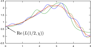
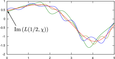
Figure 1. Real part (left) and imaginary part (right) of $L_{x}(1/2+it,\chi_{7a})$

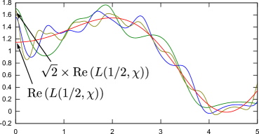
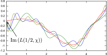
Figure 2. Real part (left) and imaginary part (right) of $L_{x}(1/2+it,\chi_{7b})$

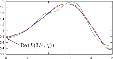
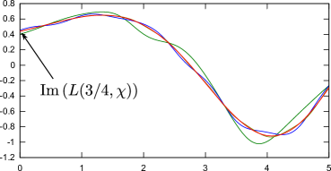
Figure 3. Real part (left) and imaginary part (right) of $L_{x}(3/4+it,\chi_{7a})$

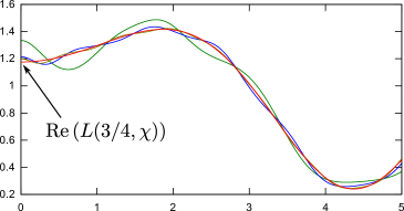
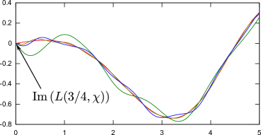
Figure 4. Real part (left) and imaginary part (right) of $L_{x}(3/4+it,\chi_{7b})$

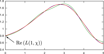
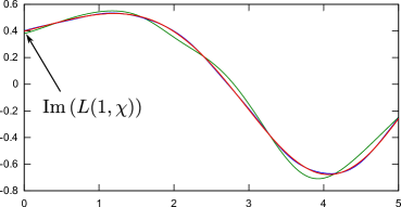
Figure 5. Real part (left) and imaginary part (right) of $L_{x}(1+it,\chi_{7a})$

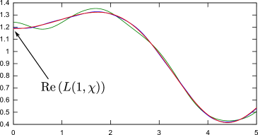
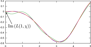
Figure 6. Real part (left) and imaginary part (right) of $L_{x}(1+it,\chi_{7b})$

Denote by $p_{n}$ the $n$-th prime number. Figures 1, 2, 3, 4, 5 and 6 show the datum for the values

$$L_{x}\left(\frac{1}{2}+it,\,\chi\right),\qquad L_{x}\left(\frac{3}{4}+it,\,\chi\right),\qquad L_{x}\left(1+it,\,\chi\right)$$

for $x=p_{10}$ (green), $x=p_{100}$ (blue), $x=p_{1000}$ (yellow) and $\infty$ (red). Figures 1, 3 and 5 are for $\chi_{7a}$, and Figures 2, 4 and 6 for $\chi_{7b}$. As $t\to 0$, we apparently see that $L_{x}\left(1/2+it,\,\chi\right)\to L(1/2,\chi)$ for $\chi^{2}\neq{\bf 1}$, that $L_{x}\left(1/2+it,\,\chi\right)\to\sqrt{2}L(1/2,\chi)$ for $\chi^{2}={\bf 1}$, and that $L_{x}\left(3/4+it,\,\chi\right)\to L(3/4,\chi)$, $L_{x}\left(1+it,\,\chi\right)\to L(1,\chi)$ for both cases $\chi^{2}={\bf 1}$ and $\chi^{2}\not={\bf 1}$. This supports the DRH (Conjecture 2).

We introduce the following error function in order to estimate the speed of convergence for $L_{x}(s,\chi)$:

$$\delta L_{x}(s,\chi)=\begin{cases}\left|\frac{L_{x}(s,\chi)-\sqrt{2}L(s,\chi)}{\sqrt{2}L(s,\chi)}\right|&(s=1/2\ and\ \chi^{2}={\bf 1})\\[8.0pt] \left|\frac{L_{x}(s,\chi)-L(s,\chi)}{L(s,\chi)}\right|&(otherwise)\end{cases}\,.$$

Figure 7 shows the values of $\delta L_{x}(s,\chi)$. When we approximate the error function as $\delta L_{x}(s,\chi)\sim x^{-\alpha}$, the exponents are determined so that they fit the numerical results (Table 2). We see the speed of convergence becomes faster as $s$ gets larger, if $s$ is real.

$s$		$\alpha\ (\chi_{7a})$		$\alpha\ (\chi_{7b})$
$1/2$		0.1167		0.1978
$3/4$		0.3814		0.3106
$1$		0.6389		0.6302

Table 2. Exponents of $\delta L_{x}(s,\chi)\sim x^{-\alpha}$ for $\chi_{7a}$ and $\chi_{7b}$.

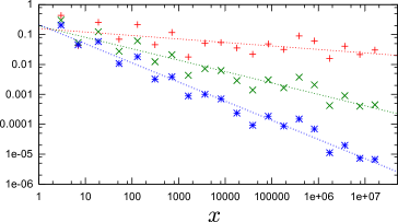
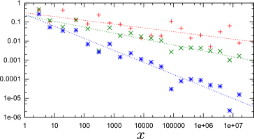
Figure 7. $\delta L_{x}(s,\chi)$ for $s=1/2$ (red), $s=3/4$ (green) and $s=1$ (blue) with $\chi_{7a}$ (left) and $\chi_{7b}$ (right)

4. Finite Size Scaling

In this section, we show another special feature that $L_{x}(s,\chi)$ has. Since $L_{x}(s,\chi)$ is a finite Euler product, it obviously has no zeros on the critical line. Nevertheless, $L_{x}(s,\chi)$ gives a certain sequence of complex numbers, which seemingly grows up to the nontrivial zeros of $L(s,\chi)$, as $x\to\infty$. In other words, the finite partial Euler product $L_{x}(s,\chi)$ already “knows” the nontrivial zeros of $L(s,\chi)$.

In Figures 10, 10 and 10, the blue curves show the values

$$\rho_{x}(t)=\frac{1}{\pi}{\rm Im}\frac{d}{dt}\log L_{x}\left(\frac{1}{2}+it,\,\chi\right)$$ (3)

with $x=p_{1000}$ for $\chi_{3}$, $\chi_{7a}$, $\chi_{7b}$, respectively. The red curves are $|L\left(\frac{1}{2}+it,\,\chi\right)|$. This function (3) is an analog of the eigenvalue density function in random matrix theory. The Riemann zeta function on the critical line $s=1/2+it$ can be seen as a characteristic polynomial of a certain infinite dimensional matrix [KS, BH]: With the Riemann-Siegel theta function

$$\vartheta(t)={\rm Im}\log\Gamma\left(\frac{it}{2}+\frac{1}{4}\right)-\frac{t}{2}\log\pi\,,$$

the function $Z(t)=e^{i\vartheta(t)}\zeta\left(\frac{1}{2}+it\right)$ turns out to be real. This is because the completed $\zeta$-function

$$\xi(s)=\frac{s(s-1)}{2}\pi^{-s/2}\Gamma\left(\frac{s}{2}\right)\zeta(s)$$

is real on ${\rm Re}(s)=1/2$ due to the functional equation $\xi(s)=\xi(1-s)$. Dirichlet $L$-functions also have similar representations. The real function $Z(t)$ changes its signature at nontrivial zeros of the Riemann zeta function. Thus $Z(t)$ is expressed as a regularized product

$$\prod_{j=1}^{\infty}\raise 6.45831pt\hbox{\scriptsize reg}\,(t-t_{j})$$

where $t_{j}$ satisfies $\zeta\left(\frac{1}{2}+it_{j}\right)=0$. This means the argument of $Z(t)$ jumps by $\pi$ at the zeros. Therefore when we define the density function of the nontrivial zeros on the critical line as

$$\rho(t) = \sum_{j=1}^{\infty}\delta(t-t_{j})$$

$$= \frac{1}{\pi}{\rm Im}\sum_{j=1}^{\infty}\frac{1}{t-t_{j}}$$

$$= \frac{1}{\pi}{\rm Im}\frac{d}{dt}\log\prod_{j=1}^{\infty}\raise 6.45831pt\hbox{\scriptsize reg}\,(t-t_{j}),$$

the function (3) should converge to this density function in the limit of $x\to\infty$, up to the factor coming from $\vartheta(t)$. Here we simply write the delta function as $\delta(x)=\frac{1}{\pi}{\rm Im}\frac{1}{x}$, which is originally represented as $\delta(x)=\lim_{\epsilon\to 0^{+}}\pm\frac{1}{\pi}{\rm Im}\frac{1}{x\mp i\epsilon}$.

Apparently the location of the zeros of $|L(\frac{1}{2}+it,\,\chi)|$ agrees to that of the peaks of $\rho_{x}(t)$ in Figures 10, 10 and 10. This suggests that a finite set of first few primes already “knows” the nontrivial zeros of $L(s,\,\chi)$, and that the Euler product would be meaningful beyond the boundary. We also observe that the blue curve oscillates near $t=0$ if and only if $\chi^{2}={\bf 1}$.

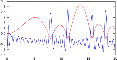
Figure 8. $\rho_{x}(t)$ for $\chi_{3}$

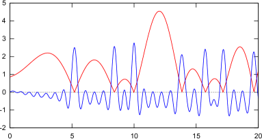
Figure 9. $\rho_{x}(t)$ for $\chi_{7a}$

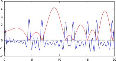
Figure 10. $\rho_{x}(t)$ for $\chi_{7b}$

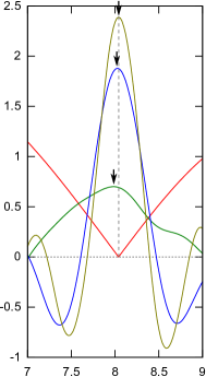
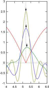
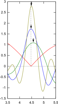
Figure 11. Peaks in $\rho(t)$ with the smallest zero for $\chi_{3}$ (left), $\chi_{7a}$ (center) and $\chi_{7b}$ (right)

Figure 11 shows how the peaks of $\rho(t)$ with the smallest zero in Figures 10, 10 and 10 get closer to the zeros of $L(s,\,\chi)$ for $x=p_{10}$ (green), $x=p_{100}$ (blue), $x=p_{1000}$ (yellow). We see these peaks getting higher and narrower, and approaching the Dirac delta function. This kind of scaling behavior is often found in critical phenomena associated with some phase transitions. Especially, in this case, the situation is similar to percolation theory [SA].

Figures 14, 14 and 14 indicate the values

$$R_{x}(t)=\frac{1}{\pi}{\rm Im}\log L_{x}\left(\frac{1}{2}+it,\,\chi\right)$$

for $\chi_{3}$, $\chi_{7a}$, $\chi_{7b}$, respectively, for $x=p_{10}$ (green), $x=p_{100}$ (blue), $x=p_{1000}$ (yellow) and $\infty$ (red). This also seems to reflect the property of DRH. The green, blue and yellow curves appear to converge to the red one more smoothly only when $\chi^{2}\neq{\bf 1}$ (Figure 14). In the other two cases, the curves oscillate many times near the origin.

The leaps in the red curves correspond to the zeros of $L(s,\chi)$. We normalize that the jumps at zeros are equal to one. This reflects the conjecture that the multiplicity of such zeros should be all one. In other words, if we express their derivatives by the Dirac delta function, the coefficients are one.

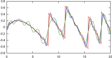
Figure 12. $R_{x}(t)$ for $\chi_{3}$

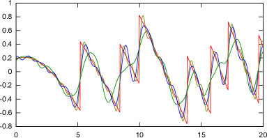
Figure 13. $R_{x}(t)$ for $\chi_{7a}$

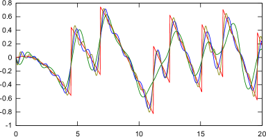
Figure 14. $R_{x}(t)$ for $\chi_{7b}$

We define another function $N_{x}(t)$ from $R_{x}(t)$ by subtracting the contribution of the $L$-function versions of the Riemann-Siegel theta function. This counts the number of the nontrivial zeros on the critical line in the limit of $x\to\infty$. Figures 17, 17 and 17 show the values of $N_{x}(t)$ for $\chi_{3}$, $\chi_{7a}$, $\chi_{7b}$, respectively. The panels of Figures 18, 19, 20 show $N_{x}(t)$ around the smallest nontrivial zeros of the $L$-functions with $x=p_{10}$ (green), $x=p_{50}$ (light blue), $x=p_{100}$ (blue), $x=p_{500}$ (purple), $x=p_{1000}$ (yellow) and $x=\infty$ (red). As the case of $R_{x}(t)$, we see a sharp step structure as the cut-off parameter $x$ getting larger.

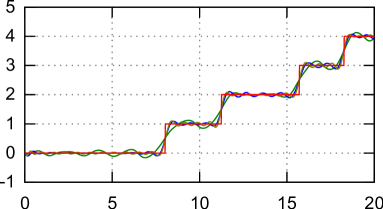
Figure 15. $N_{x}(t)$ for $\chi_{3}$

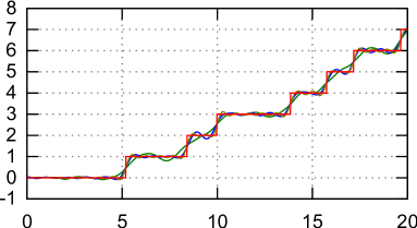
Figure 16. $N_{x}(t)$ for $\chi_{7a}$

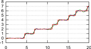
Figure 17. $N_{x}(t)$ for $\chi_{7b}$

These figures also tell us that the values ${\rm Im}\log L(\frac{1}{2}+it)$ are almost stable for nontrivial zeros $\frac{1}{2}+it$ of the $L$-function, no matter how many prime numbers we take into account. This suggests that the nontrivial zeros are analogs of the critical points in statistical mechanics, which are stable to the finite-size correction.

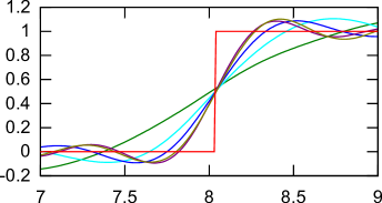
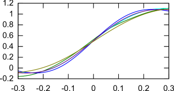
Figure 18. $N_{x}(t)$ (left) and $\tilde{N}_{x}(z)$ (right) for $\chi_{3}$

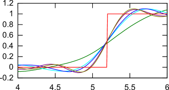
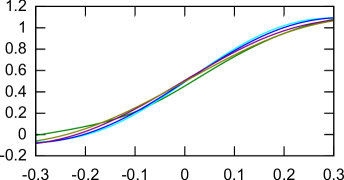
Figure 19. $N_{x}(t)$ (left) and $\tilde{N}_{x}(z)$ (right) for $\chi_{7a}$

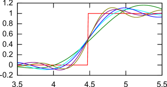
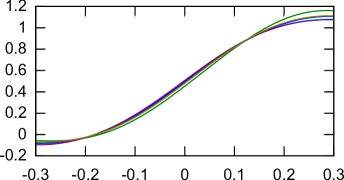
Figure 20. $N_{x}(t)$ (left) and $\tilde{N}_{x}(z)$ (right) for $\chi_{7b}$

character		$t_{1}$		$\lambda$
$\chi_{3}$		8.0397…		0.217
$\chi_{7a}$		5.1981…		0.193
$\chi_{7b}$		4.4757…		0.151

Table 3. Numerically evaluated exponents around the smallest zeros $\frac{1}{2}+it_{1}$ for $\chi_{3}$, $\chi_{7a}$ and $\chi_{7b}$

To examine the analogy to critical phenomena in statistical mechanics, we shall check the scaling property around the critical point. Being the smallest zero $\frac{1}{2}+it_{1}$, we define the scaling variable

$$z=\frac{t-t_{1}}{t_{1}}x^{\lambda}\,.$$

Correspondingly we introduce a scaled function $\tilde{N}_{x}(z)$, defined as $N_{x}(t)=\tilde{N}_{x}(z=\frac{t-t_{1}}{t_{1}}x^{\lambda})$. Right panels of Figures 18, 19 and 20 show the values of $\tilde{N}_{x}(z)$. By choosing a proper exponent $\lambda$, all the curves are almost approximated by only one curve. This means that the dependence on the cut-off parameter $x$ appears only in the form of the scaling variable $z$. This scaling behavior supports the similarity to the critical phenomena.

Table 3 shows the numerical values of the smallest zeros of the $L$-functions and the corresponding exponents for $\chi_{3}$, $\chi_{7a}$ and $\chi_{7b}$. These exponents are numerically determined by fitting the curves of $\tilde{N}_{x}(z)$ by changing the parameter $x=10,50,100,500,1000$.

In the case of the ordinary critical phenomena, there is only one critical point. On the other hand, there are infinitely many zeros on the critical line of the $L$-function, which are analogs of the critical point. Thus, even if we focus on only the smallest zero, as discussed in this study, there should be correction to its scaling bahavior from such other zeros: we have to take care of the scaling property for others simultaneously.

References

[A] H. Akatsuka:
The Euler product for the Riemann zeta-function on the
critical line. (preprint, 2012)
[G] D. Goldfeld:
Sur les produits partiels eulériens attachés aux courbes
elliptiques,
C. R. Acad. Sci. Paris Sér. I Math. 294 (1982) 471–474.
[Gr]
A. Grothendieck:
Cohomologie -adique et fonctions ,
Seminaire de Geometrie Algebrique du Bois-Marie 1965-66, SGA 5,
Springer Lecture Notes in Math. 589 (1977).
[J]
F. H. Jackson:
On -definite integrals,
Q. J. Pure Appl. Math. 41 (1910) 193–203.
[SA]
D. Stauffer and A. Aharony:
Introduction to percolation theory, CRC press, 1994.
[T] E. C. Titchmarsh:
The theory of the Riemann zeta function,
Oxford University Press, 1987.
[W1] A. Weil:
Sur les courbes algébriques et les variétés qui s’en
déduisent,
Actualités Sci. Ind. 1041 =
Publ. Inst. Math. Univ. Strasbourg 7 (1945), Hermann,
1948.