Isospin-breaking corrections to superallowed Fermi $\beta$-decay in isospin- and angular-momentum-projected nuclear Density Functional Theory

Abstract

Background

The superallowed $\beta$-decay rates provide stringent constraints on physics beyond the Standard Model of particle physics. To extract crucial information about the electroweak force, small isospin-breaking corrections to the Fermi matrix element of superallowed transitions must be applied.

Purpose

We perform systematic calculations of isospin-breaking corrections to superallowed $\beta$-decays and estimate theoretical uncertainties related to the basis truncation, time-odd polarization effects related to the intrinsic symmetry of the underlying Slater determinants, and to the functional parametrization.

Methods

We use the self-consistent isospin- and angular-momentum-projected nuclear density functional theory employing two density functionals derived from the density independent Skyrme interaction. Pairing correlations are ignored. Our framework can simultaneously describe various effects that impact matrix elements of the Fermi decay: symmetry breaking, configuration mixing, and long-range Coulomb polarization.

Results

The isospin-breaking corrections to the $I=0^{+},T=1\rightarrow I=0^{+},T=1$ pure Fermi transitions are computed for nuclei from $A$=10 to $A$=98 and, for the first time, to the Fermi branch of the $I,T=1/2\rightarrow I,T=1/2$ transitions in mirror nuclei from $A$=11 to $A$=49. We carefully analyze various model assumptions impacting theoretical uncertainties of our calculations and provide theoretical error bars on our predictions.

Conclusions

The overall agreement with empirical isospin-breaking corrections is very satisfactory. Using computed isospin-breaking corrections we show that the unitarity of the CKM matrix is satisfied with a precision better than 0.1%.

I Introduction

By studying isotopes with enhanced sensitivity to fundamental symmetries, nuclear physicists can test various aspects of the Standard Model in ways that are complementary to other sciences. For example, a possible explanation for the observed asymmetry between matter and anti-matter in the universe could be studied by searching for a permanent electric dipole moment larger than Standard Model predictions in heavy radioactive nuclei that have permanent octupole shapes. Likewise, the superallowed $\beta$-decays of a handful of rare isotopes with similar numbers of protons and neutrons, in which both the parent and daughter nuclear states have zero angular momentum and positive parity, are the unique laboratory to study the strength of the weak force.

What makes these pure vector-current-mediated (Fermi) decays so useful for testing the Standard Model is the hypothesis of the conserved vector current (CVC), that is, independence of the vector current on the nuclear medium. The consequence of the CVC hypothesis is that the product of the statistical rate function $f$ and partial half-life $t$ for the superallowed $I=0^{+},T=1\rightarrow I=0^{+},T=1$ Fermi $\beta$-decay should be nucleus independent and equal to:

$$ft=\frac{K}{G_{\rm V}^{2}|M_{\rm F}^{(\pm)}|^{2}}={\rm const}\,,$$ (1)

where $K/(\hbar c)^{6}=2\pi^{3}\hbar\ln 2/(m_{\rm e}c^{2})^{5}=8120.2787(11)\times 10^{-10}$ GeV^-4s is a universal constant; $G_{\rm V}$ stands for the vector coupling constant for semi-leptonic weak interaction, and $M_{\rm F}^{(\pm)}$ is the nuclear matrix element of the isospin rising or lowering operator $\hat{T}_{\pm}$.

The relation (1) does not hold exactly and must be slightly amended by introducing a set of radiative corrections to the $ft$-values, and a correction to the nuclear matrix element due to isospin-symmetry breaking:

$$|M_{\rm F}^{(\pm)}|^{2}=2(1-\delta_{\rm C}),$$ (2)

see Refs. Hardy and Towner (2005a); *(Har05a); Towner and Hardy (2008); Hardy and Towner (2009); Towner and Hardy (2010a) and references cited therein. Since these corrections are small, of the order of a percent, they can be approximately factorized and arranged in the following way:

$${\cal F}t\equiv ft(1+\delta_{\rm R}^{\prime})(1+\delta_{\rm NS}-\delta_{\rm C})=\frac{K}{2G_{\rm V}^{2}(1+\Delta^{\rm V}_{\rm R})},$$ (3)

with the left-hand side being nucleus independent. In Eq. (3), $\Delta^{\rm V}_{\rm R}=2.361(38)$% stands for the nucleus-independent part of the radiative correction Marciano and Sirlin (2006), $\delta_{\rm R}^{\prime}$ is a transition-dependent ($Z$-dependent) but nuclear-structure-independent part of the radiative correction Marciano and Sirlin (2006); Towner and Hardy (2008), and $\delta_{\rm NS}$ denotes the nuclear-structure-dependent part of the radiative correction Towner (1994); Towner and Hardy (2008).

In spite of theoretical uncertainties in the evaluation of the radiative and isospin-symmetry-breaking corrections, the superallowed $\beta$-decay is the most precise source of experimental information for determining the vector coupling constant $G_{\rm V}$, and provides us with a stringent test of the CVC hypothesis. In turn, it is also the most precise source of the matrix element $V_{\rm ud}=G_{\rm V}/G_{\rm\mu}$ of the Cabibbo-Kobayashi-Maskawa (CKM) three-generation quark mixing matrix Cabibbo (1963); Kobayashi and Maskawa (1973); Towner and Hardy (2008); Nakamura and Particle Data Group (2010). This is so because the leptonic coupling constant, $G_{\mu}/(\hbar c)^{3}=1.16637(1)\times 10^{-5}$  GeV^-2, is well known from the muon decay Nakamura and Particle Data Group (2010).

The advantage of the superallowed $\beta$-decay strategy results from the fact that, within the CVC hypothesis, $V_{\rm ud}$ can be extracted by averaging over several transitions in different nuclei. For precise tests of the Standard Model, only these transitions that have $ft$-values known with a relative precision better than a fraction of a percent are acceptable. Currently, 13 “canonical” transitions spreading over a wide range of nuclei from $A=10$ to $A=74$ meet this criterion (have $ft$-values measured with accuracy of order of 0.3% or better) and are used to evaluate the values of $G_{\rm V}$ and $V_{\rm ud}$ Towner and Hardy (2008).

In this work we concentrate on the isospin-breaking (ISB) corrections $\delta_{\rm C}$, which were already computed by various authors, using a diverse set of nuclear models Damgaard (1969); Towner and Hardy (2008); Sagawa et al. (1996); Liang et al. (2009); Auerbach (2009); Satuła et al. (2011, 2011, 2011); Rafalski and Satuła (2012). The standard in this field has been set by Towner and Hardy (HT) Towner and Hardy (2008) who used the nuclear shell-model to account for the configuration mixing effect, and the mean-field (MF) approach to account for a radial mismatch of proton and neutron single-particle (s.p.) wave functions caused by the Coulomb polarization. In this study, which constitutes an extension of our earlier work Satuła et al. (2011), we use the isospin- and angular-momentum-projected density functional theory (DFT). This method can account, in a rigorous quantum-mechanical way, for spontaneous symmetry-breaking (SSB) effects, configuration mixing, and long-range Coulomb polarization effects.

Our paper is organized as follows. The model is described in Sec. II. The results of calculations for ISB corrections to the superallowed ${0^{+}\rightarrow 0^{+}}$ Fermi transitions are summarized in Sec. III. The ISB corrections to the Fermi matrix elements in mirror-symmetric ${T=1/2}$ nuclei are discussed in Sec. IV. Section V studies a particular case of the Fermi decay of ³²Cl. Finally, the summary and perspectives are given in Sec. VI.

II The model

The success of the self-consistent DFT approach to mesoscopic systems Yannouleas and Landman (2007) in general, and specifically to atomic nuclei Frauendorf (2001); Bender et al. (2003); Satuła and Wyss (2005), has its roots in the SSB mechanism that incorporates essential short-range (pairing) and long-range (spatial) correlations within a single deformed Slater determinant. The deformed states provide a basis for the symmetry-projected DFT approaches, which aim at including beyond-mean-field correlations through the restoration of broken symmetries by means of projection techniques Ring and Schuck (1980).

II.1 Isospin- and angular-momentum-projected DFT approach

The building block of the isospin- and angular-momentum-projected DFT approach employed in this study is the self-consistent deformed MF state $|\varphi\rangle$ that violates both the rotational and isospin symmetries. While the rotational invariance is of fundamental nature and is broken spontaneously, the isospin symmetry is violated both spontaneously and explicitly by the Coulomb interaction between protons. The strategy is to restore the rotational invariance, remove the spurious isospin mixing caused by the isospin SSB effect, and retain only the physical isospin mixing due to the electrostatic interaction Satuła et al. (2009, 2010). This is achieved by a rediagonalization of the entire Hamiltonian, consisting the isospin-invariant kinetic energy and Skyrme force and the isospin-non-invariant Coulomb force, in a basis that conserves both angular momentum and isospin.

To this end, we first find the self-consistent MF state $|\varphi\rangle$ and then build a normalized angular-momentum- and isospin-conserving basis $|\varphi;\,IMK;\,TT_{z}\rangle$ by using the projection method:

$$|\varphi;\,IMK;\,TT_{z}\rangle=\frac{1}{\sqrt{N_{\varphi;IMK;TT_{z}}}}\hat{P}^{T}_{T_{z},T_{z}}\hat{P}^{I}_{M,K}|\varphi\rangle,$$ (4)

where $\hat{P}^{T}_{T_{z},T_{z}}$ and $\hat{P}^{I}_{M,K}$ stand for the standard isospin and angular-momentum projection operators:

$$\hat{P}^{T}_{T_{z},T_{z}} = \frac{2T+1}{2}\int_{0}^{\pi}d^{T}_{T_{z}T_{z}}(\beta_{T})\hat{R}(\beta_{T})\sin\beta_{T}\,d\beta_{T},$$ (5)

$$\hat{P}^{I}_{M,K} = \frac{2I+1}{8\pi^{2}}\int D^{I\,*}_{MK}(\Omega)\hat{R}(\Omega)\,d\Omega,$$ (6)

where, $\hat{R}(\beta_{T})=e^{-i\beta_{T}\hat{T}_{y}}$ is the rotation operator about the $y$-axis in the isospace, $d^{T}_{T_{z}T_{z}}(\beta_{T})$ is the Wigner function, and $T_{z}=(N-Z)/2$ is the third component of the total isospin $\bm{T}$. As usual, $\hat{R}(\Omega)=e^{-i\gamma\hat{J}_{z}}e^{-i\beta\hat{J}_{y}}e^{-i\alpha\hat{J}_{z}}$ is the three-dimensional rotation operator in space, $\Omega=(\alpha,\beta,\gamma)$ are the Euler angles, $D^{I}_{MK}(\Omega)$ is the Wigner function, and $M$ and $K$ denote the angular-momentum components along the laboratory and intrinsic $z$-axis, respectively Ring and Schuck (1980); Varshalovich et al. (1988). Note that unpaired MF states $|\varphi\rangle$ conserve the third isospin component $T_{z}$; hence, the one-dimensional isospin projection suffices.

The set of states (4) is, in general, overcomplete because the $K$ quantum number is not conserved. This difficulty is overcome by selecting first the subset of linearly independent states known as collective space Ring and Schuck (1980), which is spanned, for each $I$ and $T$, by the so-called natural states $|\varphi;\,IM;\,TT_{z}\rangle^{(i)}$ Dobaczewski et al. (2009); Zduńczuk et al. (2007). The entire Hamiltonian – including the ISB terms – is rediagonalized in the collective space, and the resulting eigenfunctions are:

$$|n;\,\varphi;\,IM;\,T_{z}\rangle=\sum_{i,T\geq|T_{z}|}a^{(n;\varphi)}_{iIT}|\varphi;\,IM;TT_{z}\rangle^{(i)},$$ (7)

where the index $n$ labels the eigenstates in ascending order according to their energies. The amplitudes $a^{(n;\varphi)}_{iIT}$ define the degree of isospin mixing through the so-called isospin-mixing coefficients (or isospin impurities), determined for a given $n$th eigenstate as:

$$\alpha_{\rm C}^{n}=1-\sum_{i}|a^{(n;\varphi)}_{iIT}|^{2},$$ (8)

where the sum of norms corresponds to the isospin $T$ dominating in the wave function $|n;\,\varphi;\,IM;\,T_{z}\rangle$.

One of the advantages of the projected DFT as compared to the shell-model-based approaches Ormand and Brown (1995); Towner and Hardy (2008) is that it allows for a rigorous quantum-mechanical evaluation of the Fermi matrix element using the bare isospin operators:

$$\hat{T}_{\pm}=\frac{1}{2}\sum_{k=1}^{A}\left(\hat{\tau}^{(k)}_{x}\pm i\hat{\tau}^{(k)}_{y}\right)\equiv\mp\frac{1}{2}\hat{T}_{1\,\pm 1},$$ (9)

where $\hat{T}_{1\,\pm 1}$ denotes the rank-one covariant one-body spherical-tensor operators in the isospace, see the discussion in Ref. Miller and Schwenk (2008); *(Mil09). Indeed, noting that each $m$th eigenstate (7) can be uniquely decomposed in terms of the original basis states (4),

$$|m;\varphi;\,IM;\,T_{z}\rangle=\sum_{K,T}\,f_{KT}^{(\varphi;\,m,I)}\hat{P}^{T}_{T_{z},T_{z}}\,\hat{P}^{I}_{M,K}|\varphi\rangle,$$ (10)

with microscopically determined mixing coefficients $f_{KT}^{(\varphi;\,m,I)}$, the expression for the Fermi matrix element between the parent state $|m;\,\varphi;\,IM;\,T_{z}\rangle$ and daughter state $|n;\,\psi;\,IM;\,T_{z}\pm 1\rangle$ can be written as:

$$\langle m;\,\varphi;\,IM;\,T_{z}|\hat{T}_{\mp}|n;\,\psi;\,IM;\,T_{z}\pm 1\rangle=\pm\frac{1}{2}\sum_{TT^{\prime}}\sum_{KK^{\prime}}f_{KT}^{(\varphi;\,m,I)\,*}\,f_{K^{\prime}T^{\prime}}^{(\psi;\,n,I)}\langle\varphi|\hat{P}^{T}_{T_{z},T_{z}}\hat{T}_{1\,\mp 1}\hat{P}^{T^{\prime}}_{T_{z}\pm 1,T_{z}\pm 1}\hat{P}^{I}_{K,K^{\prime}}|\psi\rangle$$

$$=\pm\frac{2I+1}{16\pi^{2}}\sum_{TT^{\prime}}\sum_{KK^{\prime}}f_{KT}^{(\varphi;\,m,I)\,*}\,f_{K^{\prime}T^{\prime}}^{(\psi;\,n,I)}\int d\Omega\,D^{I\,*}_{KK^{\prime}}(\Omega)\langle\varphi|\hat{P}^{T}_{T_{z},T_{z}}\hat{T}_{1\,\mp 1}\hat{P}^{T^{\prime}}_{T_{z}\pm 1,T_{z}\pm 1}|{\tilde{\psi}}\rangle,$$ (11)

where tilde indicates the Slater determinant rotated in space: $|{\tilde{\psi}}\rangle=|\psi(\Omega)\rangle=\hat{R}(\Omega)|\psi\rangle$. The matrix element appearing on the right-hand side of Eq. (II.1) can be expressed through the transition densities that are basic building blocks of the multi-reference DFT Sheikh and Ring (2000); Egido and Robledo (2001); Lacroix et al. (2009); Satuła et al. (2010). Indeed, with the aid of the identity

$$\hat{P}^{T}_{K,M}\hat{T}_{\lambda\,\mu}\hat{P}^{T^{\prime}}_{M^{\prime},K^{\prime}}=C^{TM}_{T^{\prime}M^{\prime}\,\lambda\mu}\sum_{\nu=-\lambda}^{\lambda}C^{TK}_{T^{\prime}K-\nu\,\lambda\nu}\hat{T}_{\lambda\nu}\hat{P}^{T^{\prime}}_{K-\nu,K^{\prime}},$$ (12)

which results from the general transformation rule for spherical tensors under rotations or isorotations,

$$\hat{R}(\Omega)\hat{T}_{\lambda\mu}{\hat{R}(\Omega)}^{\dagger}=\sum_{\mu^{\prime}}D^{\lambda}_{\mu^{\prime}\mu}(\Omega)\hat{T}_{\lambda\mu^{\prime}},$$ (13)

the matrix element entering Eq. (II.1) can be expressed as:

$$\langle\varphi|\hat{P}^{T}_{T_{z},T_{z}}\hat{T}_{1\,\mp 1}\hat{P}^{T^{\prime}}_{T_{z}\pm 1,T_{z}\pm 1}|{\tilde{\psi}}\rangle=C^{TT_{z}}_{T^{\prime}T_{z}\pm 1\,1\mp 1}\sum_{\nu}C^{TT_{z}}_{T^{\prime}T_{z}-\nu\,1\nu}\langle\varphi|\hat{T}_{1\,\nu}\hat{P}^{T^{\prime}}_{T_{z}-\nu,T_{z}\pm 1}|{\tilde{\psi}}\rangle.$$ (14)

For unpaired Slater determinants considered here, the double integral over the isospace Euler angles in Eq. (II.1) can be further reduced to a one-dimensional integral over the angle $\beta_{T}$ using the identity

$$\hat{T}_{\lambda\mu}e^{i\alpha\hat{T}_{z}}=e^{-i\alpha\mu}e^{i\alpha\hat{T}_{z}}\hat{T}_{\lambda\mu},$$ (15)

which is the one-dimensional version of the transformation rule (13) valid for rotations around the $Oz$ axis in the isospace. The final expression for the matrix element in Eq. (14) reads:

$$\langle\varphi|\hat{T}_{1\,\nu}\hat{P}^{T^{\prime}}_{T_{z}-\nu,T_{z}\pm 1}|{\tilde{\psi}}\rangle=\frac{2T^{\prime}+1}{2}\int_{0}^{\pi}d\beta_{T}\,\sin\beta_{T}\,d^{T^{\prime}}_{T_{z}-1,T_{z}\pm 1}\langle\varphi|\hat{T}_{1\,\nu}e^{-i\beta_{T}\hat{T}_{y}}|{\tilde{\psi}}\rangle$$

$$=(-1)^{\nu}\frac{2T^{\prime}+1}{2}\int_{0}^{\pi}d\beta_{T}\sin\beta_{T}d^{T^{\prime}}_{T_{z}-1,T_{z}\pm 1}{\cal N}(\Omega,\beta_{T})\int d^{3}{\bm{r}}\,{\tilde{\tilde{\rho}}}_{1\,-\nu}(\Omega,\beta_{T},{\bm{r}}),$$ (16)

where ${\tilde{\tilde{\rho}}}_{1\nu}(\Omega,\beta_{T},{\bm{r}})$ is the isovector transition density, and the double-tilde sign indicates that the right Slater determinant used to calculate this density is rotated both in space as well as in isospace: $|{\tilde{\tilde{\psi}}}\rangle=\hat{R}(\beta_{T})\hat{R}(\Omega)|\psi\rangle$. The symbol ${\cal N}(\Omega,\beta_{T})=\langle\varphi|\hat{R}(\beta_{T})\hat{R}(\Omega)|\psi\rangle$ denotes the overlap kernel.

Since the natural states have good isospin, the states (7) are free from spurious isospin mixing. Moreover, since the isospin projection is applied to self-consistent MF solutions, our model accounts for a subtle balance between the long-range Coulomb polarization, which tends to make proton and neutron wave functions different, and the short-range nuclear attraction, which acts in an opposite way. The long-range polarization affects globally all s.p. wave functions. Direct inclusion of this effect in open-shell heavy nuclei is possible essentially only within the DFT, which is the only no-core microscopic framework that can be used there.

Recent experimental data on the isospin impurity deduced in ⁸⁰Zr from the giant dipole resonance $\gamma$-decay studies Corsi et al. (2011) agree well with the impurities calculated using isospin-projected DFT based on modern Skyrme-force parametrizations Satuła et al. (2009, 2011). This further demonstrates that the isospin-projected DFT is capable of capturing the essential piece of physics associated with the isospin mixing.

II.2 The choice of Skyrme interaction

As discussed in Ref. Satuła et al. (2010), the isospin projection technique outlined above does not yield singularities in energy kernels; hence, it can be safely executed with all commonly used energy density functionals (EDFs). However, as demonstrated in Ref. Satuła et al. (2011), the isospin projection alone leads to unphysically large isospin mixing in odd-odd $N=Z$ nuclei. It has thus been concluded that – in order to obtain reasonable results – isospin projection must be augmented by angular-momentum projection. This not only increases the numerical effort, but also brings back the singularities in the energy kernels Satuła et al. (2011) and thus prevents one from using the modern parametrizations of the Skyrme EDFs, which all contain density-dependent terms Dobaczewski et al. (2007). Therefore, the only option Satuła et al. (2011) is to use the Hamiltonian-driven EDFs. For the Skyrme-type functionals, this leaves us with one choice: the SV parametrization Beiner et al. (1975). In order to better control the time-odd fields, the standard SV parametrization must be augmented by the tensor terms, which were neglected in the original work Beiner et al. (1975).

This density-independent parameterization of the Skyrme functional has the isoscalar effective mass as low as $\frac{m^{*}}{m}\approx 0.38$, which is required to reproduce the actual nuclear saturation properties. The unusual saturation mechanism of SV has a dramatic impact on the overall spectroscopic quality of this force, impairing such key properties like the symmetry energy Satuła et al. (2011), level density, and level ordering. These deficiencies also affect the calculated isospin mixing, which is a prerequisite for realistic estimates of $\delta_{\rm C}$. In particular, in the case of ⁸⁰Zr discussed above, SV yields $\alpha_{\rm C}\approx 2.8$%, which is considerably smaller than the mean value of $\bar{\alpha}_{\rm C}\approx 4.4\pm 0.3$% obtained by averaging over nine popular Skyrme EDFs including the MSk1, SkO’, SkP, SLy4, SLy5, SLy7, SkM^∗, SkXc, and SIII functionals, see Ref. Satuła et al. (2011) for further details. Even though the ISB corrections $\delta_{\rm C}$ are primarily sensitive to differences between isospin mixing in isobaric analogue states, the lack of a reasonable Hamiltonian-based Skyrme EDF is probably the most critical deficiency of the current formalism.

The aim of this study is (i) to provide the most reliable set of the ISB corrections that can be obtained within the current angular-momentum and isospin-projected single-reference DFT, and (ii) explore the sensitivity of results to EDF parameters, choice of particle-hole configurations, and structure of time-odd fields that correlate valence neutron-proton pairs in odd-odd $N=Z$ nuclei. In particular, to quantify uncertainties related to the Skyrme coupling constants, we have developed a new density-independent variant of the Skyrme force dubbed hereafter SHZ2, see Table 1.

The force was optimized purposefully to properties of light magic nuclei below ¹⁰⁰Sn. The coupling constants $t_{0}$, $t_{1}$,$t_{2}$,$x_{0}$ of SHZ2 were found by means of a $\chi^{2}$ minimization to experimental Audi et al. (2003) binding energies of five doubly-magic nuclei: ¹⁶O, ⁴⁰Ca, ⁴⁸Ca, ⁵⁶Ni, and ¹⁰⁰Sn. The procedure reduced the $\chi^{2}$ from $\sim 6.0$ for SV set to $\sim 3.6$ for SHZ2. Most of the nuclear matter characteristics calculated for both sets are similar. It appears, however, that the fit to light nuclei only weakly constrains the symmetry energy. The bulk symmetry energy of SHZ2 is $a_{sym}\approx 42.2$ MeV, i.e., it overestimates the accepted value $a_{sym}\approx 32\pm 2$ MeV by almost 30%. While this property essentially precludes using SHZ2 in detailed nuclear structure studies, it also creates an interesting opportunity for investigating the quenching of ISB effects due to the large isospin-symmetry-restoring components of the force.

Table 1: Skyrme parameters $t_{i},x_{i}$ ($i=0,1,2,3$), and $W$ of SV Beiner et al. (1975) (second column) and SHZ2 (third column). The last column shows relative changes of parameters (in percent). Both parametrizations use the nucleon-mass parameter of $\hbar^{2}/2m=20.73$ MeV fm². Parameters not listed are equal to zero.

param.	SV	SHZ2	change (%)
$t_{0}$	$-$1248.290	$-$1244.98830	$-$0.26
$t_{1}$	970.560	970.01156	$-$0.06
$t_{2}$	107.220	99.50197	$-$7.20
$x_{0}$	$-$0.170	0.01906	$-$111.21
$W$	150	150	$0$

II.3 Numerical details

All calculations presented below were done by using the code HFODD Dobaczewski et al. (2009); Schunck et al. (2012), version (2.48q) or higher, which includes both the angular-momentum and isospin projections. In order to obtain converged results for isospin mixing with respect to basis truncation, in our SV calculations we used $N=10$ harmonic oscillator (HO) shells for $A<40$ nuclei, 12 shells for $40\leq A<62$ nuclei, and 14 shells for $A\geq 62$ nuclei. In SHZ2 test calculations, we took $N=10$ shells for $A<40$ and $N=12$ shells for $A>40$ nuclei.

For the numerical integration over the Euler angles in space and isospace ($\alpha,\beta,\gamma;\beta_{T}$) we used the Gauss-Tchebyschev (over $\alpha$ and $\gamma$) and Gauss-Legendre (over $\beta$ and $\beta_{T}$) quadratures. We took $n_{\alpha}=n_{\beta}=n_{\gamma}=20$ and $n_{\beta_{T}}=8$ (or 10) integration points. This choice guarantees that the calculated values of $\delta_{\rm C}$ are not affected by the numerical integration error.

III ISB corrections to the superallowed $\bm{0^{+}\rightarrow 0^{+}}$ Fermi transitions

The $0^{+}\rightarrow 0^{+}$ Fermi $\beta$-decay proceeds between the ground state (g.s.) of the even-even nucleus $|I=0,T\approx 1,T_{z}=\pm 1\rangle$ and its isospin-analogue partner in the $N=Z$ odd-odd nucleus, $|I=0,T\approx 1,T_{z}=0\rangle$. The corresponding transition matrix element is:

$$M_{\rm F}^{(\pm)}=\langle I=0,T\approx 1,T_{z}=\pm 1|\hat{T}_{\pm}|I=0,T\approx 1,T_{z}=0\rangle.$$ (17)

The g.s. state $|I=0,T\approx 1,T_{z}=\pm 1\rangle$ in Eq. (17) is approximated by a projected state

$$|I=0,T\approx 1,T_{z}=\pm 1\rangle=\sum_{T\geq 1}c^{(\psi)}_{T}\hat{P}^{T}_{\pm 1,\pm 1}\hat{P}^{I=0}_{0,0}|\psi\rangle,$$ (18)

where $|\psi\rangle$ is the g.s. of the even-even nucleus obtained in self-consistent MF calculations. The state $|\psi\rangle$ is unambiguously defined by filling in the pairwise doubly degenerate levels of protons and neutrons up to the Fermi level. The daughter state $|I=0,T\approx 1,T_{z}=0\rangle$ is approximated by

$$|I=0,T\approx 1,T_{z}=0\rangle=\sum_{T\geq 0}c^{(\varphi)}_{T}\hat{P}^{T}_{0,0}\hat{P}^{I=0}_{0,0}|\varphi\rangle,$$ (19)

where the self-consistent Slater determinant $|\varphi\rangle\equiv|\bar{\nu}\otimes\pi\rangle$ (or $|\nu\otimes\bar{\pi}\rangle$) represents the so-called anti-aligned configuration, selected by placing the odd neutron and the odd proton in the lowest available time-reversed (or signature-reversed) s.p. orbits. The s.p. configuration $|\bar{\nu}\otimes\pi\rangle$ manifestly breaks the isospin symmetry as schematically depicted in Fig. 1. The isospin projection from $|\varphi\rangle$ as expressed by Eq. (19) is essentially the only way to reach the $|T\approx 1,I=0\rangle$ states in odd-odd $N=Z$ nuclei.

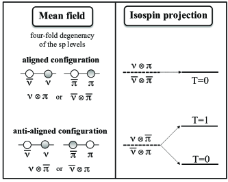
Figure 1: Left: two possible g.s. configurations of an odd-odd $N$=$Z$ nucleus, as described by the conventional deformed MF theory. These degenerate configurations are called aligned (upper) and anti-aligned (lower), depending on what levels are occupied by the valence particles. The right panel shows what happens when the isospin-symmetry is restored. The aligned configuration is isoscalar; hence, it is insensitive to the isospin projection. The anti-aligned configuration represents a mixture of $T$=0 and $T$=1 states. The isospin projection removes the degeneracy by lowering the $T$=0 level.

III.1 Shape-current orientation

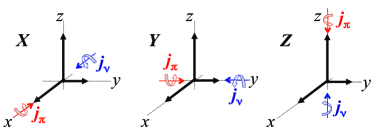
Figure 2: (Color online) Schematic illustration of relative orientations of shapes and currents in the three anti-aligned states $|\varphi_{\rm X}\rangle$ ($X$), $|\varphi_{\rm Y}\rangle$ ($Y$), and $|\varphi_{\rm Z}\rangle$ ($Z$) discussed in the text. The long ($Oz$), intermediate ($Ox$), and short ($Oy$) principal axes of the nuclear mass distribution are indicated by thick arrows. The odd-neutron ($j_{\nu}$) and odd-proton ($j_{\pi}$) angular momentum oriented along the $Ox$, $Oy$, or $Oz$ axes is shown by thin arrows. Note that in each case the total angular-momentum alignment, $j_{\nu}+j_{\pi}$, is zero.

At variance with the even-even parent nuclei, the anti-aligned configurations in odd-odd daughter nuclei are not uniquely defined. One of the reasons, which was not fully appreciated in our previous work Satuła et al. (2011), is related to the relative orientation of the nuclear shapes and currents associated with the valence neutron-proton pairs. In all signature-symmetry-restricted calculations for triaxial nuclei, such as ours, there are three anti-aligned Slater determinants with the s.p. angular momenta (alignments) of the valence protons and neutrons pointing, respectively, along the $Ox$, $Oy$, or $Oz$ axes of the intrinsic shape defined by means of the long ($Oz$), intermediate ($Ox$), and short ($Oy$) principal axes of the nuclear mass distribution. These solutions, hereafter referred to as $|\varphi_{\rm X}\rangle$, $|\varphi_{\rm Y}\rangle$, and $|\varphi_{\rm Z}\rangle$, are schematically illustrated in Fig. 2. Their properties can be summarized as follows:

• The three solutions are not linearly independent. Their Hartree-Fock (HF) binding energies may typically differ by a few hundred keV. The differences come almost entirely from the isovector correlations in the time-odd channel, as shown in the lower panel of Fig. 3 for a representative example of ³⁴Cl. Let us stress that these poorly-known correlations may significantly impact the ISB corrections, as shown in the upper panel of Fig. 3.

• The type of the isovector time-odd correlations captured by the HF solutions depends on the relative orientation of the nucleonic currents with respect to the nuclear shapes. Solutions oriented perpendicular to the long axis, $|\varphi_{\rm X}\rangle$ and $|\varphi_{\rm Y}\rangle$, are usually similar to one another (they yield identical correlations for axial systems) and differ from $|\varphi_{\rm Z}\rangle$, oriented parallel to the long axis, which captures more correlations due to the current-current time-odd interactions.

• The three $|T=1,I=0^{+}\rangle$ states projected from the $|\varphi_{\rm X}\rangle$, $|\varphi_{\rm Y}\rangle$, and $|\varphi_{\rm Z}\rangle$ Slater determinants differ in energy by only a few tens of keV, see the lower panel of Fig. 3. Hence, energy-wise, they represent the same physical solution, differing only slightly due to the polarization effects originating from different components of the time-odd isovector fields. However, since these correlations are completely absent in the even-even parent nuclei, they strongly impact the calculated $\delta_{\rm C}$. The largest differences in $\delta_{\rm C}$ have been obtained for $A=34$ and $A=74$ systems, see Fig. 3 and Tables 2 and 3.

• Symmetry-unrestricted calculations always converge to the signature-symmetry-conserving solution $|\varphi_{Z}\rangle$ which, rather surprisingly, appears to be energetically unfavored (except for ¹⁸F). In spite of our persistent efforts, no self-consistent tilted-axis solutions have been found.

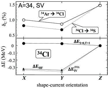
Figure 3: Upper panel: the ISB corrections $\delta_{\rm C}$ for the $0^{+}\rightarrow 0^{+}$ superallowed $\beta$-decays ³⁴Ar$\rightarrow^{34}$Cl (open circles) and ³⁴Cl$\rightarrow^{34}$S (full circles) determined for the shape-current orientations $X$, $Y$, and $Z$ depicted schematically in Fig. 2. Lower panel: differences between the energies of the $X$ and $Y$ configurations, and the $Z$ configuration in ³⁴Cl. Full triangles correspond to the total HF energies and open triangles correspond to contributions from the time-odd isovector channel. Full dots show the total energy differences obtained for the angular-momentum and isospin-projected states.

III.2 Nearly degenerate $\bm{K}$-orbitals

Owing to an increased density of s.p. Nilsson levels in the vicinity of the Fermi surface for nearly spherical nuclei, there appears another type of ambiguity in choosing the Slater determinants representing the anti-aligned configurations. Within the set of nuclei studied in this work, this ambiguity manifests itself particularly strongly in ⁴²Sc, where we deal with four possible anti-aligned MF configurations built on the Nilsson orbits originating from the spherical $\nu f_{7/2}$ and $\pi f_{7/2}$ sub-shells. These configurations can be labeled in terms of the quantum number $K$ as $|\nu\bar{K}\otimes\pi K\rangle$ with $K=1/2$, 3/2, 5/2, and 7/2.

In the extreme shell-model picture, each of these states contains all the $T=1$ and $I$=0, 2, 4, and 6 components. Within the projected DFT picture, owing to configuration-dependent polarizations in time-odd and time-even channels, the situation is more complicated because the Slater determinants $|\nu\bar{K}\otimes\pi K\rangle$ corresponding to different $K$-values are no longer degenerate. Consequently, for each angular momentum $I$, one obtains four different linearly-dependent solutions. Calculations show that in all $I$=0 and $T\approx 1$ states of interest, the isospin mixing $\alpha_{\rm C}$ is essentially independent of the choice of the initial Slater determinant. In contrast, the calculated ISB corrections $\delta_{\rm C}$ and energies depend on $K$, see Fig. 4.

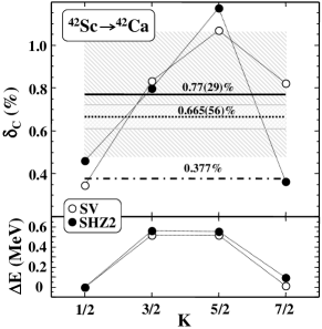
Figure 4: Top: the ISB corrections to the ⁴²Sc$\rightarrow$⁴²Ca superallowed $\beta$-transition, calculated using SV (circles) and SHZ2 (dots) forces by projecting the $|\nu\bar{K}\otimes\pi K\rangle$ configurations in ⁴²Sc for $K=1/2$, 3/2, 5/2, and 7/2. From top to bottom, horizontal lines mark (i) the average ISB correction using SV (thick solid line); (ii) the value of Ref. Towner and Hardy (2008) (dotted line); and (iii) $\delta_{\rm C}$ of Ref. Liang et al. (2009). Shaded regions mark the related uncertainties. Bottom: projected energies of states $|K;I=0^{+},T\approx 1\rangle$ in ⁴²Sc obtained from the configurations $|\nu\bar{K}\otimes\pi K\rangle$, relative to the projected energy of the $K=1/2$ state.

III.3 Theoretical uncertainties and error analysis

Based on the discussion presented in Secs. III.1 and III.2, the recommended calculated values of $\delta_{\rm C}$ for the superallowed $0^{+}\rightarrow 0^{+}$ $\beta$-decay are determined by averaging over three relative orientations of shapes and currents. Only in the case of $A=42$, we adopt for $\delta_{\rm C}$ an arithmetic mean over the four configurations associated with different $K$-orbitals.

To minimize uncertainties in $\alpha_{\rm C}$ and $\delta_{\rm C}$ associated with the truncation of HO basis in HFODD, we used different HO spaces in different mass regions, cf. Sec. II.3. With this choice, the resulting systematic errors due the basis cut-off should not exceed $\sim 10$%. To illustrate the dependence of $\delta_{\rm C}$ on the number of HO shells, Fig. 5 shows the case of the superallowed ⁴⁶V$\rightarrow$⁴⁶Ti transition obtained by projecting from the $|\varphi_{\rm Z}\rangle$ solution in ⁴⁶V. In this case, the parent and daughter nuclei are axial, which allows us to reduce the angular-momentum projection to one-dimension and extend the basis size up to $N=20$ HO shells.

With increasing $N$, $\delta_{\rm C}$ increases, and asymptotically it reaches the value of $0.8096(12)$%. This limiting value is about 6.7% larger than the value of $0.7587$% obtained for $N=12$ shells, that is, for a basis used to compute the $42\leq A\leq 54$ cases. For $62\leq A\leq 74$ nuclei, which were all found to be triaxial, we have used $N=14$ shells. The further increase of basis size is practically impossible. Nonetheless, as seen in Fig. 5, a rate of increase of $\delta_{\rm C}$ slows down exponentially with $N$, which supports our 10% error estimate due to the basis truncation.

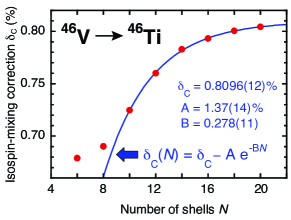
Figure 5: (Color online) The convergence of the ISB correction $\delta_{\rm C}$ to the ⁴⁶V$\rightarrow$⁴⁶Ti superallowed $\beta$-decay versus the number of oscillator shells considered.

The total error of the calculated value of $\delta_{\rm C}$ includes the standard deviation from the averaging, $\sigma_{n}$, and the assumed 10% uncertainty due to the basis size: $\Delta(\delta_{\rm C})=\sqrt{\sigma_{n}^{2}+(0.1\delta_{\rm C})^{2}}$. The same prescription for $\Delta(\delta_{\rm C})$ was also used in the test calculations with SHZ2, even though a slightly smaller HO basis was employed in that case.

For $A=38$ nuclei, our model predicts the unusually large correction $\delta_{\rm C}\approx 10$%. The origin of a very different isospin mixing obtained for odd-odd and even-even members of this isobaric triplet is not fully understood. Most likely, it is a consequence of the poor spectroscopic properties of SV. Indeed, as a result of an incorrect balance between the spin-orbit and tensor terms in SV, the $2s_{1/2}$ subshell is shifted up in energy close to the Fermi surface. This state is more sensitive to time-odd polarizations than other s.p. states around ⁴⁰Ca core, see Table I in Ref. Zalewski et al. (2008). The calculated equilibrium deformations $(\beta_{2},\gamma)$ of the $T_{z}\pm 1$ and $T_{z}=0$ $A=38$ isobaric triplet are very similar, around (0.090, 60^∘). In the following, the ³⁸K$\rightarrow$³⁸Ar transition is excluded from the calculation of the $V_{\rm ud}$ matrix element.

III.4 The survey of ISB corrections in $10\leq A\leq 74$ nuclei

Table 2: Results of calculations for the superallowed transitions measured experimentally. Shown are: the empirical $ft$-values Towner and Hardy (2010a); SV values of $\delta_{\rm C}$ calculated by projecting from the $|\varphi_{\rm X}\rangle,|\varphi_{\rm Y}\rangle$, and $|\varphi_{\rm Z}\rangle$ Slater determinants, see Sec. III.1; recommended mean $\delta_{\rm C}^{{\rm(SV)}}$ corrections (see Sec. III.3) and the corresponding ${\cal F}t$-values; empirical $\delta_{\rm C}^{{\rm(exp)}}$ corrections calculated by using Eq. (23); contributions coming from the individual transitions to the $\chi^{2}$ budget in the confidence-level test; mean $\delta_{\rm C}^{{\rm(SHZ2)}}$ corrections and the corresponding ${\cal F}t$-values.

Parent	$ft$		$\delta_{\rm C}^{\rm(X)}$	$\delta_{\rm C}^{\rm(Y)}$	$\delta_{\rm C}^{\rm(Z)}$		$\delta_{\rm C}^{{\rm(SV)}}~{}$	${\cal F}t~{}~{}~{}~{}~{}$		$\delta_{\rm C}^{{\rm(exp)}}~{}$	$\chi^{2}_{i}$		$\delta_{\rm C}^{{\rm(SHZ2)}}~{}~{}$	${\cal F}t~{}~{}~{}~{}~{}$
nucleus	(s)		(%)	(%)	(%)		(%)	(s)		(%)			(%)	(s)
$T_{z}=-1:$
10C	3041.7(43)		0.559	0.559	0.823		0.65(14)	3062.1(62)		0.37(15)	3.7		0.462(65)	3067.8(49)
14O	3042.3(11)		0.303	0.303	0.303		0.303(30)	3072.3(21)		0.36(06)	0.8		0.480(48)	3066.9(24)
22Mg	3052.0(70)		0.243	0.243	0.417		0.301(87)	3080.5(75)		0.62(23)	1.9		0.342(49)	3079.2(72)
34Ar	3052.7(82)		0.865	0.997	1.475		1.11(29)	3056(12)		0.63(27)	3.1		1.08(42)	3057(15)
$T_{z}=0:$
26Al	3036.9(09)		0.308	0.308	0.494		0.370(95)	3070.5(31)		0.37(04)	0.0		0.307(62)	3072.5(23)
34Cl	3049.4(11)		0.809	0.679	1.504		1.00(38)	3060(12)		0.65(05)	48.4		0.83(50)	3065(15)
42Sc	3047.6(12)		—	—	—		0.77(27)	3069.2(85)		0.72(06)	0.5		0.70(32)	3071(10)
46V	3049.5(08)		0.486	0.486	0.759		0.58(14)	3074.6(47)		0.71(06)	4.5		0.375(96)	3080.9(35)
50Mn	3048.4(07)		0.460	0.460	0.740		0.55(14)	3074.1(47)		0.67(07)	3.1		0.39(13)	3079.2(45)
54Co	3050.8(10)		0.622	0.622	0.671		0.638(68)	3074.0(32)		0.75(08)	2.0		0.51(20)	3078.0(66)
62Ga	3074.1(11)		0.925	0.840	0.881		0.882(95)	3090.0(42)		1.51(09)	44.0		0.49(11)	3102.3(45)
74Rb	3084.9(77)		2.054	1.995	1.273		1.77(40)	3073(15)		1.86(27)	0.1		0.90(22)	3101(11)
							$\overline{{\cal F}t}=$	3073.6(12)		$\chi^{2}=$	112.2		$\overline{{\cal F}t}=$	3075.0(12)
							$|V_{\rm ud}|=$	0.97397(27)		$\chi_{d}^{2}=$	10.2		$|V_{\rm ud}|=$	0.97374(27)
								0.99935(67)						0.99890(67)

Table 3: Similar as in Table 2, except for the unmeasured transitions.

Parent	$\delta_{\rm C}^{\rm(X)}$	$\delta_{\rm C}^{\rm(Y)}$	$\delta_{\rm C}^{\rm(Z)}$		$\delta_{\rm C}^{\rm(SV)}$		$\delta_{\rm C}^{\rm(SHZ2)}$
nucleus	(%)	(%)	(%)		(%)		(%)
$T_{z}=-1:$
18Ne	2.031	1.064	1.142		1.41(46)		0.72(30)
26Si	0.399	0.399	0.597		0.47(10)		0.529(77)
30S	1.731	1.260	1.272		1.42(26)		0.98(21)
$T_{z}=0:$
18F	1.819	0.956	0.987		1.25(42)		0.42(24)
22Na	0.255	0.255	0.535		0.35(14)		0.216(86)
30P	1.506	0.974	1.009		1.16(27)		0.60(20)
66As	0.956	0.925	1.694		1.19(38)		0.64(12)
70Br	1.654	1.479	1.429		1.52(18)		1.10(52)

The results of our calculations are collected in Tables 2 and 3, and in Fig. 6. In addition, Fig. 7 shows the differences, $\delta_{\rm C}^{({\rm SV})}-\delta_{\rm C}^{({\rm HT})}$, between our results and those of Ref. Towner and Hardy (2008). In spite of clear differences between SV and HT, which can be seen for specific transitions including those for $A=10$, 34, and 62, both calculations reveal a similar increase of $\delta_{\rm C}$ versus $A$, at variance with the RPA calculations of Ref. Liang et al. (2009), which also yield systematically smaller values.

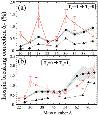
Figure 6: (Color online) ISB corrections to the superallowed $0^{+}\rightarrow 0^{+}$ $\beta$-decays calculated for (a) $T_{z}=-1\rightarrow T_{z}=0$ and (b) $T_{z}=0\rightarrow T_{z}=1$ transitions. Our adopted values from Table 2 (circles with error bars) are compared with ISB corrections from Refs. Towner and Hardy (2008) (dots, shaded band marks errors) and Liang et al. (2009) (triangles).

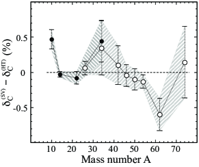
Figure 7: Differences between the ISB corrections to the twelve accurately measured superallowed $0^{+}\rightarrow 0^{+}$ $\beta$-transitions (excluding $A$=38) calculated in this work with SV and those of HT Towner and Hardy (2008). Circles and dots mark the $T_{z}=-1\rightarrow T_{z}=0$ and $T_{z}=0\rightarrow T_{z}=1$ decays, respectively. The errors, calculated as $\sqrt{(\Delta\delta_{\rm C}^{\rm(SV)})^{2}+(\Delta\delta_{\rm C}^{\rm(HT)})^{2}}$, are shown by shaded bands.

The ISB corrections used for further calculations of $V_{\rm ud}$ are collected in Table 2. Let us recall that our preference is to use the averaged corrections and that the ³⁸K$\rightarrow$³⁸Ar transition has been disregarded. All other ingredients needed to compute the ${\cal F}t$-values, including radiative corrections $\delta_{\rm R}^{\prime}$ and $\delta_{\rm NS}$, are taken from Ref. Towner and Hardy (2008), and the empirical $ft$-values are taken from Ref. Towner and Hardy (2010a). For the sake of completeness, these empirical $ft$-values are also listed in Table 2.

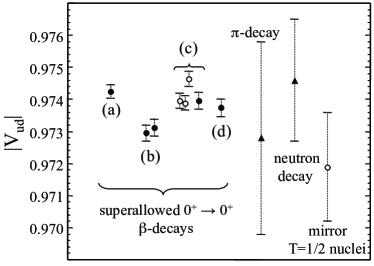
Figure 8: The matrix element $|V_{\rm ud}|$ deduced from the superallowed $0^{+}\rightarrow 0^{+}$ $\beta$-decay (dots) for different sets of the $\delta_{\rm C}$ corrections calculated in: (a) Ref. Towner and Hardy (2008); (b) Ref. Liang et al. (2009) with NL3 and DD-ME2 Lagrangians; this work, using the averaged values of $\delta_{\rm C}$ with (c) SV and (d) SHZ2 functionals. Gray circles show ISB corrections with SV calculated at fixed shape-current orientations $X$, $Y$, and $Z$ (from left to right). Triangles mark values obtained from the pion-decay Počanić et al. (2004) and neutron-decay Nakamura and Particle Data Group (2010) studies. The open circle shows $|V_{\rm ud}|$ deduced from the $\beta$-decays in the $T=1/2$ mirror nuclei Naviliat-Cuncic and Severijns (2009a)

.

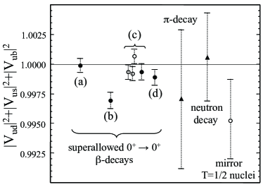
Figure 9: Similar as in Fig. 8 except for the unitarity condition (20).

In the error budget of the resulting ${\cal F}t$-values listed in Table 2, apart from errors in the $ft$ values and radiative corrections, we also included the uncertainties estimated for the calculated values of $\delta_{\rm C}$, see Sec. III.3. To conform with HT, the average value $\overline{{\cal F}t}=3073.6(12)$s was calculated by using the Gaussian-distribution-weighted formula. However, unlike HT, we do not apply any further corrections to $\overline{{\cal F}t}$. This leads to $|V_{\rm ud}|=0.97397(27)$, which agrees very well with both the HT result Towner and Hardy (2008), $|V_{\rm ud}^{{\rm(HT)}}|=0.97418(26)$, and the central value obtained from the neutron decay $|V_{\rm ud}^{(\nu)}|=0.9746(19)$ Nakamura and Particle Data Group (2010). A survey of the $|V_{\rm ud}|$ values deduced by using different methods is given in Fig. 8. By combining the value of $|V_{\rm ud}|$ calculated here with those of $|V_{\rm us}|=0.2252(9)$ and $|V_{\rm ub}|=0.00389(44)$ of the 2010 Particle Data Group Nakamura and Particle Data Group (2010), one obtains

$$|V_{\rm ud}|^{2}+|V_{\rm us}|^{2}+|V_{\rm ub}|^{2}=0.99935(67),$$ (20)

which implies that the unitarity of the first row of the CKM matrix is satisfied with a precision better than 0.1%. A survey of the unitarity condition (20) is shown in Fig. 9.

It is worth noting that by using $\delta_{\rm C}$ values corresponding to the fixed current-shape orientations ($|\varphi_{\rm X}\rangle$, $|\varphi_{\rm Y}\rangle$, or $|\varphi_{\rm Z}\rangle$) instead of their average, one still obtains compatible results for $|V_{\rm ud}|$ and unitarity condition (20), see Figs. 8 and 9. Moreover, the value of $|V_{\rm ud}|$ obtained by using SHZ2 is only $\approx$0.024 % smaller than the SV result, see Table 2. This is an intriguing result, which indicates that an increase of the bulk symmetry energy – that tends to restore the isospin symmetry – is partly compensated by other effects. The most likely origin of this compensation mechanism is due to the time-odd spin-isospin mean fields, which are poorly constrained by the standard fitting protocols of Skyrme EDFs Osterfeld (1992); Bender et al. (2002); Zduńczuk et al. (2005). For instance, if one compares the Landau-Migdal parameters characterizing the spin-isospin time-odd channels Osterfeld (1992); Bender et al. (2002); Zduńczuk et al. (2005) of SV ($g_{0}=0.57$, $g_{0}^{\prime}=0.31$, $g_{1}=0.46$, $g_{1}^{\prime}=0.46$) and SHZ2 ($g_{0}=0.27$, $g_{0}^{\prime}=0.30$, $g_{1}=0.47$, $g_{1}^{\prime}=0.47$) one notices that these two functionals differ by a factor of two in the scalar-isoscalar Landau-Migdal parameter $g_{0}$.

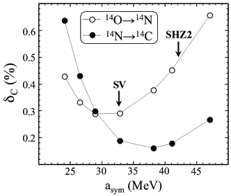
Figure 10: ISB corrections for ¹⁴O$\rightarrow^{14}$N and ¹⁴N$\rightarrow^{14}$C superallowed $0^{+}\rightarrow 0^{+}$ $\beta$-decays calculated for a set of SV-based Skyrme forces with systematically varied $x_{0}$ parameter, which affects the bulk asymmetry energy coefficient $a_{sym}$ and spin-spin fields. The arrows indicate $x_{0}$ values corresponding to SV and SHZ2.

To illustrate the compensation mechanism related to the bulk symmetry energy and $g_{0}$, in Fig. 10 we plot $\delta_{\rm C}$ for the ¹⁴O$\rightarrow^{14}$N$\rightarrow^{14}$C super-allowed $0^{+}\rightarrow 0^{+}$ transitions as functions of the bulk symmetry parameter $a_{sym}$ for a set of SV-based Skyrme forces with systematically varied $x_{0}$ parameter. At a functional level, $x_{0}$ affects only two Skyrme coupling constants (see e.g. Appendix A in Ref. Bender et al. (2003)):

$$C_{1}^{\rho} = -\frac{1}{4}t_{0}\left(\frac{1}{2}+x_{0}\right)-\frac{1}{24}t_{3}\left(\frac{1}{2}+x_{3}\right)\rho_{0}^{\alpha},$$ (21)

$$C_{0}^{s} = -\frac{1}{4}t_{0}\left(\frac{1}{2}-x_{0}\right)-\frac{1}{24}t_{3}\left(\frac{1}{2}-x_{3}\right)\rho_{0}^{\alpha}.$$ (22)

The coupling constant $C_{1}^{\rho}$ influences the isovector part of the bulk symmetry energy Satuła et al. (2006) while $C_{0}^{s}$ affects $g_{0}$. The ISB correction in Fig. 10 exhibits a minimum indicating the presence of the compensation effect. Similar effect was calculated for the $A=34$ transitions. Hence, it is safe to state that our exploratory calculations are indicative of the interplay between the symmetry energy and time-odd fields.

III.5 Confidence level test

In this section, we present results of the confidence-level (CL) test proposed in Ref. Towner and Hardy (2010a). The CL test is based on the assumption that the CVC hypothesis is valid up to at least $\pm 0.03$%, which implies that a set of structure-dependent corrections should produce statistically consistent set of ${\cal F}t$-values. Assuming the validity of the calculated corrections $\delta_{\rm NS}$ Towner (1994), the empirical ISB corrections can be defined as:

$$\delta_{\rm C}^{{\rm(exp)}}=1+\delta_{\rm NS}-\frac{\overline{{\cal F}t}}{ft(1+\delta_{\rm R}^{\prime})}.$$ (23)

By the least-square minimization of the appropriate $\chi^{2}$, and treating the value of $\overline{{\cal F}t}$ as a single adjustable parameter, one can attempt to bring the set of empirical values $\delta_{\rm C}^{{\rm(exp)}}$ as close as possible to the set of $\delta_{\rm C}$.

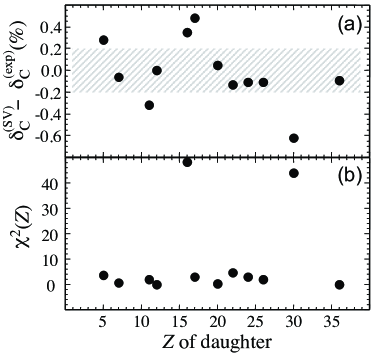
Figure 11: Top: differences between the calculated ISB corrections and empirical values resulting from the CL test of Ref. Towner and Hardy (2010a). The shaded area of width $\pm 0.2$% is added in order to better visualize the differences. Bottom: contributions from individual transitions to the $\chi^{2}$ budget. Note the particularly large contributions from the ³⁴Cl$\rightarrow^{34}$S and ⁶²Ga $\rightarrow^{62}$Zn transitions that deteriorate the CL test. See text for details.

The empirical ISB corrections deduced in this way are tabulated in Table 2 and illustrated in Fig. 11. Table 2 also lists individual contributions to the $\chi^{2}$ budget. The obtained $\chi^{2}$ per degree of freedom ($n_{d}=11$) is $\chi^{2}/n_{d}=10.2$. This number is twice as large as that quoted in our previous work Satuła et al. (2011), because of the large uncertainty of $\delta_{\rm C}$ for the ³⁴Cl$\rightarrow^{34}$S transition. Other than that, both previous and present calculations have difficulty in reproducing the strong increase for $A=62$. Our $\chi^{2}/n_{d}$ is also higher than the perturbative-model values reported in Ref. Towner and Hardy (2010a) ($\chi^{2}/n_{d}=1.5$), shell model with Woods-Saxon (SM-WS) radial wave functions (0.4) Towner and Hardy (2008), shell model with Hartree-Fock (SM-HF) radial wave functions (2.0) Ormand (1996); Hardy and Towner (2009), Skyrme-Hartree-Fock with RPA (2.1) Sagawa et al. (1996) , and relativistic Hartree-Fock plus RPA model (RHF-RPA) Liang et al. (2009), which yields $\chi^{2}/n_{d}=1.7$.

It is worth noting that after disregarding the two transitions that strongly violate the CVC hypothesis, ³⁴Cl$\rightarrow^{34}$S and ⁶²Ga$\rightarrow^{62}$As that, and then performing a new CL test for the remaining ten transitions ($n_{d}=9$), the normalized $\chi^{2}$ drops to 1.9. Within this restricted set of data, the calculated $|V_{ud}|=0.97420(28)$ and unitarity condition 0.99978(68) almost perfectly match the results of Ref. Towner and Hardy (2008).

III.6 ISB corrections in $78\leq A\leq 98$ nuclei

Our projected DFT approach can be used to predict isospin mixing in heavy nuclei. The calculated ISB corrections and $Q$-values in $78\leq A\leq 98$ nuclei are listed in Table 4. The values of $\delta_{\rm C}$ are also shown in Fig. 12. Note that the predicted ISB corrections are here considerably smaller than those in $A$=70 and $A$=74 nuclei, see Tables 2 and 3. For the sake of comparison, Fig. 12 also shows predictions of Ref. Petrovici et al. (2008) for the ⁸²Nb$\rightarrow^{82}$Zr transition using the VAMPIR approach with either charge-independent Bonn A potential or charge-dependent Bonn CD potential. Note that our prediction is only slightly below the Bonn A result and significantly lower than the Bonn CD value. For the sake of completeness, it should be mentioned that our $Q_{\beta}$-value of 10.379 MeV for this transition agrees well with $Q_{\beta}=10.496$ MeV (Bonn A) and 10.291 MeV (Bonn CD) calculated within the VAMPIR approach.

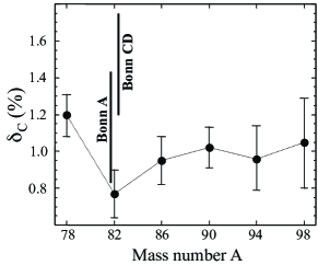
Figure 12: The ISB corrections to the superallowed $0^{+}\rightarrow 0^{+}$ transitions in heavy nuclei calculated in the present work (full dots). Vertical bars mark the ISB corrections to the ⁸²Nb$\rightarrow$⁸²Zr transition calculated in Ref. Petrovici et al. (2008) by using the VAMPIR formalism with the charge-independent Bonn A and charge-dependent Bonn CD interactions.

Table 4: Results of calculations for the superallowed $\beta$-decays in $78\leq A\leq 98$ nuclei: the isospin impurities in the parent and daughter nuclei; $\delta_{\rm C}$ for different shape-current orientations; averaged (recommended) $\delta_{\rm C}$; calculated equilibrium deformations $\beta_{2}$ and $\gamma$; and $Q_{\beta}$-values calculated here and estimated from the extrapolated masses of Ref. Audi et al. (2003).

				$\alpha_{\rm C}^{{\rm(P)}}$	$\alpha_{\rm C}^{{\rm(D)}}$		$\delta_{\rm C}^{{\rm(X)}}$	$\delta_{\rm C}^{{\rm(Y)}}$	$\delta_{\rm C}^{{\rm(Z)}}$	$\delta_{\rm C}^{{\rm(SV)}}$		$\beta_{2}^{{\rm(SV)}}$	$\gamma^{{\rm(SV)}}$		$Q_{\beta}^{{\rm(th)}}$	$Q_{\beta}^{{\rm(exp)}}$
				(%)	(%)		(%)	(%)	(%)	(%)			(deg)		(MeV)	(MeV)
$T_{z}=0$	$\rightarrow$	$T_{z}=1$
78Y	$\rightarrow$	78Sr		2.765	0.976		1.20	1.19	1.20	1.20(12)		0.004	60.0		10.471	10.650#
82Nb	$\rightarrow$	82Zr		3.099	1.408		0.70	0.91	0.70	0.77(13)		0.036	60.0		10.379	11.220#
86Tc	$\rightarrow$	86Mo		3.337	1.518		0.89	0.89	1.08	0.95(13)		0.122	0.0		10.965	11.350#
90Rh	$\rightarrow$	90Ru		3.525	1.608		0.99	0.99	1.09	1.02(11)		0.161	0.0		11.465	12.090#
94Ag	$\rightarrow$	94Pd		3.674	1.689		0.86	0.86	1.17	0.96(18)		0.136	0.0		11.896	13.050#
98In	$\rightarrow$	98Cd		3.805	1.771		0.89	0.89	1.36	1.05(25)		0.057	0.0		12.343	13.730#

Our calculated values of $\delta_{\rm C}$ are in heavy nuclei considerably smaller than those obtained from a perturbative expression Damgaard (1969); Towner et al. (1977); Towner and Hardy (2010a):

$$\delta_{\rm C}=0.002645\frac{Z^{2}}{A^{2/3}}(n+1)(n+\ell+3/2)\,{\rm(\%)},$$ (24)

where $n$ and $\ell$ denote the number of radial nodes and angular momentum of the valence s.p. spherical wave function, respectively. Indeed, assuming the valence $1p_{1/2}$ state in $A=78$, Eq. (24) yields $\delta_{\rm C}$=1.54%. In heavier nuclei, where the spherical valence state is $0g_{9/2}$, Eq. (24) gives $\delta_{\rm C}$ values that increase smoothly from 1.30% in $A=82$ to 1.64% in $A=98$.

IV ISB corrections to the Fermi matrix elements in mirror-symmetric $\bm{T=1/2}$ nuclei

Transitions between the isobaric analogue states in mirror nuclei $|T=1/2,I,T_{z}=-1/2\rangle$$\rightarrow$$|T=1/2,I,T_{z}=+1/2\rangle$ offer an alternative way to extract the ${\cal F}t$-values Severijns et al. (2008) and $V_{ud}$ Naviliat-Cuncic and Severijns (2009a, b). Those transitions are mixed Fermi and Gamow-Teller, meaning that they are mediated by both the vector and axial-vector currents. Hence, the extraction of $V_{ud}$ requires – in addition to lifetimes and $Q$-values – measuring another observable, such as the beta-neutrino correlation coefficient, beta-asymmetry, or neutrino-asymmetry parameter Severijns et al. (2006); Towner and Hardy (2010b). Moreover, the method depends on the radiative and ISB corrections to both the Fermi and Gamow-Teller matrix elements. In spite of these difficulties, current precision of determination of $V_{ud}$ using the mirror-decay approach is similar to that offered by neutron-decay experiments Nakamura and Particle Data Group (2010); Naviliat-Cuncic and Severijns (2009a, b), see also Figs. 8 and 9.

Within our projected-DFT model, we performed systematic calculations of ISB corrections to the Fermi matrix elements, $\delta_{\text{C}}^{\text{V}}$, covering the mirror transitions in all $11\leq A\leq 49$ nuclei. Calculations were based on the Slater determinants corresponding to the lowest-energy, unrestricted-symmetry HF solutions. If the unrestricted-symmetry calculations did not converge, the projection was applied to the constrained HF solutions with imposed signature symmetry. These two types of solutions differ, in particular, in relative shape-current orientation, which also varies with $A$ depending on the s.p. orbit occupied by an unpaired nucleon. It should be underlined, however, that the HF solutions corresponding to the $\beta$-decay partners were always characterized by the same orientation of the odd-particle alignment with respect to the body-fixed reference frame. All calculations discussed in this section were performed by using the full basis of $N=12$ HO shells and the SV force.

Table 5: Results of calculations for $|T=1/2,I,T_{z}=-1/2\rangle$$\rightarrow$$|T=1/2,I,T_{z}=+1/2\rangle$ $\beta$-decays between mirror nuclei: theoretical spin and parity assignments; isospin-mixing coefficients in the parent and daughter nuclei; ISB corrections calculated in this work (asterisks denote results obtained within unrestricted-symmetry calculations); ISB corrections of Ref. Severijns et al. (2008); quadrupole equilibrium deformation parameters in the parent nuclei; and theoretical and experimental $Q_{\beta}$ values.

				$I^{\pi}$		$\alpha_{\rm C}^{{\rm(P)}}$	$\alpha_{\rm C}^{{\rm(D)}}$		$\delta^{{\text{V}}\,{\rm(SV)}}_{\rm C}$	$\delta_{\rm C}^{{\text{V}}\,{\rm(S)}}$		$\beta_{2}^{{\rm(SV)}}$	$\gamma^{{\rm(SV)}}$		$Q_{\beta}^{{\rm(th)}}$	$Q_{\beta}^{{\rm(exp)}}$
						(%)	(%)		(%)	(%)			(deg)		(MeV)	(MeV)
11C	$\rightarrow$	11B		$\frac{3}{2}^{-}$		0.001	0.003		0.077	0.928		0.320	43.8		1.656	1.983
13N	$\rightarrow$	13C		$\frac{1}{2}^{-}$		0.008	0.001		0.139	0.271		0.210	59.1		1.888	2.221
15O	$\rightarrow$	15N		$\frac{1}{2}^{-}$		0.012	0.002		0.127	0.181		0.003	0.0		2.446	2.754
17F	$\rightarrow$	17O		$\frac{5}{2}^{+}$		0.020	0.031		0.167	0.585		0.014	0.0		2.496	2.761
						0.019	0.029		∗0.178	0.585		0.064	60.0		2.499
19Ne	$\rightarrow$	19F		$\frac{1}{2}^{+}$		0.036	0.034		0.365	0.415		0.321	0.0		2.928	3.239
21Na	$\rightarrow$	21Ne		$\frac{3}{2}^{+}$		0.047	0.052		0.307	0.348		0.434	0.0		3.229	3.548
23Mg	$\rightarrow$	23Na		$\frac{3}{2}^{+}$		0.064	0.070		0.340	0.293		0.434	0.0		3.587	4.057
25Al	$\rightarrow$	25Mg		$\frac{5}{2}^{+}$		0.073	0.058		0.503	0.461		0.444	1.6		3.683	4.277
27Si	$\rightarrow$	27Al		$\frac{5}{2}^{+}$		0.074	0.073		0.472	0.312		0.343	47.7		4.250	4.813
29P	$\rightarrow$	29Si		$\frac{1}{2}^{+}$		0.123	0.113		0.694	0.976		0.332	54.4		4.399	4.943
31S	$\rightarrow$	31P		$\frac{5}{2}^{+}$		0.163	0.164		0.504	0.715		0.315	0.0		4.855	5.396
33Cl	$\rightarrow$	33S		$\frac{3}{2}^{+}$		0.177	0.160		0.644	0.865		0.258	33.5		5.002	5.583
35Ar	$\rightarrow$	35Cl		$\frac{3}{2}^{+}$		0.186	0.182		0.576	0.493		0.209	50.4		5.482	5.966
37K	$\rightarrow$	37Ar		$\frac{3}{2}^{+}$		0.291	0.267		1.425	0.734		0.143	60.0		5.589	6.149
39Ca	$\rightarrow$	39K		$\frac{3}{2}^{+}$		0.318	0.289		∗0.392	0.855		0.034	60.0		6.084	6.531
41Sc	$\rightarrow$	41Ca		$\frac{7}{2}^{-}$		0.341	0.345		∗0.426	0.821		0.032	60.0		5.968	6.496
43Ti	$\rightarrow$	43Sc		$\frac{7}{2}^{-}$		0.376	0.380		∗0.463	0.500		0.090	60.0		6.225	6.868
45V	$\rightarrow$	45Ti		$\frac{7}{2}^{-}$		0.437	0.424		0.534	0.865		0.233	0.0		6.563	7.134
						0.438	0.427		∗0.661	0.865		0.233	0.0		6.559
47Cr	$\rightarrow$	47V		$\frac{3}{2}^{-}$		0.480	0.457		0.518	—		0.276	0.0		6.827	7.452
						0.483	0.463		∗0.710	—		0.275	0.0		6.826
49Mn	$\rightarrow$	49Cr		$\frac{5}{2}^{-}$		0.515	0.497		0.522	—		0.284	0.9		7.054	7.715
						0.518	0.499		∗0.681	—		0.284	0.0		7.053

The obtained values of the ISB corrections to the Fermi transitions,

$$\delta_{\text{C}}^{\text{V}}\equiv 1-|\langle T=\frac{1}{2},I,T_{z}=\mp\frac{1}{2}|\hat{T}_{\mp}|T=\frac{1}{2},I,T_{z}=\pm\frac{1}{2}\rangle|^{2},$$ (25)

are collected in Table 5 and illustrated in Fig. 13.

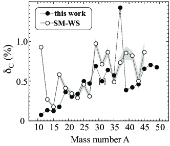
Figure 13: Full circles: calculated values of the ISB corrections to the Fermi transitions in $T=1/2$ mirror nuclei. Open circles with errors: results calculated by Severijns et al. Severijns et al. (2008).

Since the calculations were performed in a relatively large basis, the basis-cut-off-related uncertainty in $\delta_{\text{C}}^{\text{V}}$ could be reduced to approximately $5\%$, cf. Sec. III.3. Except for one case, theoretical spins and parities of decaying states were taken equal to those found in experiment: $I^{\pi}_{\text{(th)}}=I^{\pi}_{{\text{(exp)}}}$(g.s.). Only for $A=31$, no $I=1/2$ component was found in the HF wave function, and thus the lowest solution corresponding to $I^{\pi}_{\text{(th)}}=5/2^{+}$ was taken instead. It should be mentioned that, owing to the poor spectroscopic quality of SV, the projected states corresponding to $I^{\pi}_{{\text{(exp)}}}$(g.s.) are not always the lowest ones. This situation occurs for $A=19$, 25, and 45, where the lowest states have $I^{\pi}_{\text{(th)}}=5/2^{+}$, $1/2^{+}$, and $3/2^{-}$, and the corresponding $\delta_{\text{C}}^{\text{V}}$ values are 0.308 %, 0.419%, and 0.636%, respectively. A relatively strong dependence of the calculated ISB corrections on spin is worth noting. The calculations also indicate an appreciable impact of the signature-symmetry constraint on $\delta_{\text{C}}^{\text{V}}$, in particular, in the $pf$-shell nuclei with $A=45$, 47, and 49. A similar effect was calculated for the $0^{+}\rightarrow 0^{+}$ transitions, see $\delta_{\rm C}$-values at fixed shape-current orientations in Tables 2 and 3.

V The ISB correction to the Fermi decay branch in ³²Cl

The $V_{\rm ud}$ values extracted by using diverse techniques including $0^{+}\rightarrow 0^{+}$ nuclear decays, nuclear mirror decays, neutron decay, and pion decay are subject to both experimental and theoretical uncertainties. The latter pertain to calculations of radiative processes and – for nuclear methods – to the nuclear ISB effect. The uncertainties in radiative and ISB corrections affect the overall precision of $V_{\rm ud}$ at the level of a few parts per 10⁴ each Hardy and Towner (2005a); Towner and Hardy (2010b). It should be stressed, however, that the ISB contribution to the error bar of $V_{\rm ud}$ was calculated only for a single theoretical model (SM-WS). Other microscopic models, including the SM-HF Hardy and Towner (2009), RH-RPA Liang et al. (2009), and projected DFT Satuła et al. (2011), yield $\delta_{\rm C}$ corrections that may differ substantially from those obtained in SM-WS calculations.

Inclusion of the model dependence in the calculated uncertainties is expected to increase the uncertainty of $V_{\rm ud}$. According to Ref. Liang et al. (2011) the increase can reach even an order of magnitude. In our opinion, a reasonable assessment of systematic errors (due to the model dependence) cannot be done at present, as it requires the assumption that all the nuclear structure models considered are either equally reliable or their performance can be graded in an objective way.

A good way to verify the reliability of various models is to compare their predictions with empirically determined $\delta_{\rm C}$. Recently, an anomalously large value of $\delta_{\rm C}\approx 5.3(9)$% has been determined from a precision measurement of the $\gamma$ yields following the $\beta$-decay of $I=1^{+},T=1$ state in ³²Cl to its isobaric analogue state (Fermi branch) in ³²S Melconian et al. (2011). This value offers a stringent test on nuclear-structure models, because it is significantly larger than any value of $\delta_{\rm C}$ in the $A=4n+2$ nuclei. The physical reason for this enhancement can be traced back to a mixing of two close-lying $I=1^{+}$ states seen in ³²S at the excitation energies of 7002 keV and 7190 keV, respectively Ouellet and Singh (2011). The lower one is the isobaric analogue state having predominantly $T=1$ component while the higher one is primarily of $T=0$ character.

The experimental value $\delta_{\rm C}\approx 5.3(9)$% is consistent with the SM-WS calculations: $\delta_{\rm C}\approx 4.6(5)$%. In our projected-DFT approach, we also see fingerprints of the strong enhancement in $\delta_{\rm C}$ value in ³²Cl as compared to other $A=4n+2$ nuclei. Unfortunately, a static DFT approach based on projecting from a single reference state is not sufficient to give a reliable prediction. This is because, as sketched in Fig. 14, there exist ambiguities in selecting the HF reference state. In the extreme isoscalar s.p. scenario, by distributing four valence protons and neutrons over the Nilsson s.p. levels in an odd-odd nucleus, one can form two distinctively different s.p. configurations, see Fig. 14.

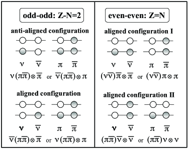
Figure 14: Schematic illustration of several possible mean-field configurations in the odd-odd $Z-N=2$ (left) and even-even $N=Z$ (right) nuclei. The pairs of proton (neutron) s.p. levels, labeled as $\pi$ and $\bar{\pi}$ ($\nu$ and $\bar{\nu}$), are assumed to be degenerated due to the intrinsic signature symmetry. The orbits $\nu$ and $\pi$ carry the signature quantum number $r=-i$ $(\alpha=1/2)$ while $\bar{\nu}$ and $\bar{\pi}$ have $r=i$ $(\alpha=-1/2)$.

The total signature of valence particles determines the total signature of the odd-odd nucleus and, in turn, an approximate angular-momentum distribution in its wave function Bengtsson and Håkansson (1978); the total additive signature $\alpha_{\rm T}\rm{(mod2)}=0(1)$ corresponds then to even (odd) spins in the wave function Bohr and Mottelson (1975). It is immediately seen that the anti-aligned configuration shown in Fig. 14 has $\alpha_{\rm T}=0$; hence, in the first approximation, it can be disregarded. In this sense, the reference wave function in ³²Cl (or, in general, in any $N-Z=\pm 2$ odd-odd nucleus) corresponds to the uniquely defined aligned state. As seen in Fig. 14, this does not hold for ³²S (or, in general, for any $N=Z$ even-even nucleus), where one must consider two possible Slater determinants having $\alpha_{\rm T}=1$, obtained by a suitable proton or neutron particle-hole excitation.

The above discussion indicates that, contrary to transitions involving the odd-odd $N=Z$ nuclei studied in Sec. III, those involving even-even $N=Z$ nuclei cannot be directly treated within the present realization of the model. To this end, the model requires enhancements including the configuration mixing (multi-reference DFT). Nevertheless, we have carried out an exploratory study by independently calculating two ISB corrections for the two configurations discussed above. These calculations proceeded in the following way:

• We select the appropriate reference configurations which, in the present case, are: $\nu[4,5,3,3]\pi[5,6,3,3]$ in ³²Cl and $\varphi_{{\rm I}}$: $\nu[5,5,3,3]\pi[4,6,3,3]$ and $\varphi_{{\rm II}}$: $\nu[4,6,3,3]\pi[5,5,3,3]$ in ³²S. The labels denote the numbers of neutrons and protons occupying the lowest Nilsson levels in each parity-signature block $(\pi,r)=(+,+i),(+,-i),(-,+i),(-,-i)$ counting from the bottom of the HF potential well, as defined in Ref. Dobaczewski and Dudek (2000).

• We determine the lowest $|I^{\pi}=1^{+},T\approx 1,T_{z}=-1\rangle$ and $|\varphi_{i};I^{\pi}=1^{+},T\approx 1,T_{z}=0\rangle$ ($i={\rm I,II}$) states by projecting onto subspaces of good angular momentum and isospin, and performing the $K$-mixing and Coulomb rediagonalization as described in Sec. II.

• Finally, we calculate matrix elements of the Fermi operator $\hat{T}_{\pm}$ and extract $\delta_{\rm C}$.

The resulting ISB corrections are $\delta_{\rm C}^{(\varphi_{{\rm I}})}=2.40(24)$% and $\delta_{\rm C}^{(\varphi_{{\rm II}})}=4.22(42)$% for the $\varphi_{I}$ and $\varphi_{{\rm II}}$ configurations, respectively. As before, we assumed a 10% error due to the basis size ($N=10$ spherical HO shells). Projections from the same configurations cranked in space to $\langle\hat{J}_{y}\rangle$ = 1$\hbar$ (see discussion in Ref. Zduńczuk et al. (2007)) leaves ISB corrections almost unaffected: $\delta_{\rm C}^{(\varphi_{\rm I})}=2.41(24)$ % and $\delta_{\rm C}^{(\varphi_{\rm{II}})}=4.30(43)$ %. A simple average value would read $\delta_{\rm C}=3.4(10)$%, which is indeed strongly enhanced as compared to the $A=4n+2$ cases. The obtained central value is smaller than both the empirical value and the SM-WS result. It is worth noting, however, that within the stated errors our mean value 3.4(10)% agrees with the SM-WS value 4.6(05)%. Whether or not the configuration-mixing calculations would provide a significant enhancement is an entirely open question.

VI Summary and perspectives

Within the recently-developed unpaired projected-DFT approach, we carried out systematic calculations of isospin mixing effects and ISB corrections to the superallowed ${0^{+}\rightarrow 0^{+}}$ Fermi decays in $10\leq A\leq 74$ nuclei and $\beta$-transitions between the isobaric analogue states in mirror ${T=1/2}$ nuclei with $11\leq A\leq 49$. Our predictions are compared with empirical values and with predictions of other theoretical approaches. Using isospin-breaking corrections computed in our model, we show that the unitarity of the CKM matrix is satisfied with a precision better than 0.1%. We also provide ISB corrections for heavier nuclei with $78\leq A\leq 98$ nuclei that can guide future experimental and theoretical studies.

We carefully analyze various model assumptions impacting theoretical uncertainties of our calculations: basis truncation, definition of the intrinsic state, and configuration selection. To assess the robustness of our results with respect to the choice of interaction, we compared SV results with predictions of the new force SHZ2 that has been specifically developed for this purpose. The comparison of SV and SHZ2 results suggest that ISB corrections are sensitive to the interplay between the bulk symmetry energy and time-odd mean-fields.

While the overall agreement with the empirical values offered by the projected-DFT approach is very encouraging, and the results are fairly robust, there is a lot of room for systematic improvements. The main disadvantages of our model in its present formulation include: (i) lack of pairing correlations; (ii) lack of ph interaction (or functional) of good spectroscopic quality; (iii) the use of a single HF reference state that cannot accommodate configuration mixing effects; (iv) ambiguities in establishing the HF reference state in odd and odd-odd nuclei caused by different possible orientations of time-odd currents with respect to total density distribution. The work on various enhancements of our model, including the inclusion of $T=0$ and $T=1$ pairing within the projected Hartree-Fock-Bogoliubov theory, better treatment of configuration mixing using the multi-reference DFT, and development of the spectroscopic-quality EDF used in projected calculations, is in progress.