Trajectories and Distribution of Interstellar Dust Grains in the Heliosphere

Abstract

The solar wind carves a bubble in the surrounding interstellar medium (ISM), known as the heliosphere. Charged interstellar dust grains (ISDG) encountering the heliosphere may be diverted around the heliopause or penetrate it depending on their charge-to-mass ratio. We present new calculations of trajectories of ISDG in the heliosphere, and the dust density distributions that result. We include up-to-date grain charging calculations using a realistic UV radiation field and full 3-D magnetohydrodynamic fluid $+$ kinetic models for the heliosphere. Models with two different (constant) polarities for the solar wind magnetic field (SWMF) are used, with the grain trajectory calculations done separately for each polarity. Small grains $a_{\mathrm{gr}}\lesssim 0.01$ µm are completely excluded from the inner heliosphere. Large grains, $a_{\mathrm{gr}}\gtrsim 1.0$ µm pass into the inner solar system and are concentrated near the Sun by its gravity. Trajectories of intermediate size grains depend strongly on the SWMF polarity. When the field has magnetic north pointing to ecliptic north, the field de-focuses the grains resulting in low densities in the inner heliosphere, while for the opposite polarity the dust is focused near the Sun. The ISDG density outside the heliosphere inferred from applying the model results to in situ dust measurements is inconsistent with local ISM depletion data for both SWMF polarities, but is bracketed by them. This result points to the need to include the time variation in the SWMF polarity during grain propagation. Our results provide valuable insights for interpretation of the in situ dust observations from Ulysses.

1 Introduction

The Sun is traveling through a magnetized, low density, partially ionized interstellar cloud (Frisch et al., 2011). The relative motion of the Sun and the cloud and the outflowing solar wind combine to produce the bow shaped heliosphere. The heliosphere consists of three distinct regions: the inner heliosphere in which the solar wind plasma expands almost freely, the inner heliosheath, which contains shocked solar wind plasma, and the outer heliosheath, which has heated and decelerated interstellar medium (ISM) plasma. If the interstellar magnetic field were small enough so that the magnetosonic speed in the surrounding ISM was below the relative speed of the solar system and the ISM, there would be a second shock marking the transition from the undisturbed ISM to the outer heliosheath. Data from a variety of sources including Voyager 1 and Voyager 2 and the Interstellar Boundary Explorer (IBEX) point to a relatively large magnetic field, $B\approx 3\,\mu$G oriented at a fairly large angle ($\sim 48\arcdeg$) relative to the upwind direction (McComas et al., 2012, and references therein). Therefore, the surrounding ISM, known as the Local Interstellar Cloud (LIC) is now thought to move subsonically relative to the Solar System and so there is no outer bow shock but rather a continuous transition beyond the heliopause that nevertheless results in heating of the plasma and an increase in the density and magnetic field strength of the ISM. The heliopause, a contact discontinuity, is the boundary between inner and outer heliosheath, and the solar wind termination shock marks the transition from the inner heliosphere to the inner heliosheath.

Though the above picture would seem to imply a clean separation of the solar wind plasma and interstellar medium, in reality there are a variety of interactions that couple components of the ISM and the solar wind throughout the heliosphere. The existence of pickup ions (PUI) is one manifestation of this coupling, since their primary source is the population of neutral interstellar atoms that are ionized by charge exchange or photoionization in the inner heliosphere and subsequently picked up by the solar wind (e.g. Gloeckler & Fisk, 2007; Zank, 1999). Interstellar dust in the solar system, observed by the Ulysses, Galileo and Cassini spacecrafts, is another example of an interstellar population modified by interaction with the heliosphere (e.g. Morfill & Grün, 1979; Frisch et al., 1999; Landgraf et al., 2000; Altobelli et al., 2007; Krüger et al., 2010). The interaction between the interstellar dust and the heliosphere, which depends on the solar wind magnetic field and grain charging by the surrounding plasma and UV radiation field, is in many ways more complex than the PUI interactions. The purpose of this study is to model the distributions of interstellar dust grains propagating into and through the heliosphere from the undisturbed ISM.

Interstellar dust (ISD) grains outside of the heliosphere span a broad range of sizes from Angstrom sizes (for polycyclic aromatic hydrocarbon dust) to several microns for the largest grains in cold molecular cloud cores (Pagani et al., 2010). The charge-to-mass ratios calculated for the larger ISD grains imply gyroradii that are large compared to the size of the heliosphere. The smaller grains, however, are tightly coupled to the magnetic field, since their gyroradii are fractions of an AU, and are swept around the heliosphere along with the magnetic field. For medium sized grains with gyroradii on the order of a few AU or so it is unclear what to expect. For these grains one needs detailed calculations of their trajectories to assess their level of density depletion or enhancement in the heliosphere and its spatial dependence.

Among the mysteries regarding the ISD observed inside of the solar system is to what extent the observed grain size distribution is representative of the undisturbed size distribution in the surrounding interstellar cloud. This point is of particular interest because the size distribution is so unusual compared to that inferred for the ISM in general from extinction of starlight, infrared emission and other evidence (Draine, 2009). The observed grains span a range from $\sim 0.05-1$ µm in size (Grün et al., 1994; Grün & Svestka, 1996) as compared to the canonical model of Mathis et al. (1977, MRN) for the interstellar dust size distribution which goes from 0.01 to 0.25 µm (for silicates, with the lower end quite uncertain). Interstellar dust models that simultaneously model grain infrared emissivity and extinction data, while satisfying the abundance constraints, require grain sizes of up to 0.8 µm, using a range of possible grain compositions and a mix of carbonaceous and silicate grains (Zubko et al., 2004). The amount of mass in the observed dust, if typical depletion of elements into grains is assumed, is marginally inconsistent with cosmic abundances (depending on the abundance set assumed) given the inferred interstellar gas density for the cloud (Slavin & Frisch, 2008). As we discuss below, however, the observed dust mass and size distribution is unlikely to closely match that in the undisturbed ISM outside of the heliosphere and so determining how to infer that initial size distribution is an important motivation for this work.

Trajectories of interstellar grains through the inner heliosphere have been calculated previously, and it was shown that the interaction of the charged grains with the solar wind magnetic field produces trajectories that depend on the phase of the solar magnetic activity cycle (e.g. Landgraf, 2000; Grogan et al., 1996; Landgraf et al., 2003; Sterken et al., 2012). Common properties of these models are the analytical treatment of the solar cycle variations of the solar wind magnetic field and a computational domain that includes a uniform source region 40–50 AU from the Sun. All these models show that grains alternately focus or de-focus with respect to the ecliptic plane, depending on the solar cycle phase. None of the previous models include the asymmetries of the full 3-D global heliosphere revealed by the Voyager termination shock crossings (Stone et al., 2008), the IBEX data including the ribbon of energetic neutral atoms (McComas et al., 2009), and the offset between the inflow direction of interstellar He⁰ and H⁰ into the heliosphere (Lallement et al., 2010). Most calculations assume a uniform grain source upwind of the Sun and without regard for the structure outer heliosphere. Czechowski & Mann (2003) have investigated the dynamics of $\sim 0.01$ µm grains in the heliosheath regions and found that such grains may stream along the heliosphere flanks, and in addition trace variations in the plasma density. Recently, Sterken et al. (2012) have presented a parameter study of grain trajectories in the time-variable inner heliosphere, within $\sim 30$ AU of the Sun for a uniform density grain source.

Our simulations of interstellar grains interacting with the heliosphere make use of global models that represent the heliosphere during either the focusing or de-focusing phase of the solar magnetic activity cycle, and provide the first study of the distribution of interstellar dust grains in the magnetically distorted global heliosphere. The heliosphere model that we use is a fully 3-D MHD-kinetic model (MHD for the ions and kinetic for the neutrals) described by Pogorelov et al. (2008). This model was created with the aim of matching all the available data on the heliosphere including the asymmetry indicated by the crossings of the termination shock by Voyager 1 and 2 (Stone et al., 2008), the H deflection plane data (Lallement et al., 2005, 2010), and the Ulysses measurement of the relative Sun-LIC velocity (Witte, 2004). It has been highly successful in predicting the direction of the interstellar magnetic field (ISMF) as inferred from data from IBEX. The region of the sky with enhanced energetic neutral atom flux detected by IBEX is known as the “ribbon” (discovered by McComas et al., 2009) and models for its production predict that its location is sensitive to the orientation of the interstellar magnetic field. The center of the ribbon arc, at $\ell=33^{\circ}\pm 4^{\circ}$, $b=55^{\circ}\pm 4^{\circ}$, is located $\sim 17\arcdeg$ from the direction of the ISMF used in our models, and $48^{\circ}$ from the interstellar gas flow direction. The angle between the ISMF and the gas flow produces a magnetically distorted heliosphere that is incorporated into the models we use. The bending of the interstellar magnetic field lines as they are wrapped around the asymmetric heliosphere has important consequences for the trajectories, particularly for grains with sizes near 0.1 µm.

While our simulations provide the first study of the interactions between interstellar dust and the global 3-D heliosphere, one of our conclusions is that the trajectories of sub-micron grains that penetrate the inner heliosheath are sensitive to the solar wind magnetic field polarity. As a result an accurate model of the propagation of these grains through the inner heliosheath regions will require a time-variable heliosphere that takes into account the variation of the SWMF because of the 22 year solar magnetic activity cycle.

2 Methods

2.1 Heliosphere Model

A big step toward constraining MHD models of the heliosphere was taken when the Voyager 1 and Voyager 2 spacecraft encountered the termination shock at different distances. These data, together with the $\sim 7.8\arcdeg$ offset between the upwind interstellar H⁰ and He⁰ directions (the so-called hydrogen deflection plane, HDP Lallement et al., 2005, 2010), and the $48\arcdeg$ angle between He⁰ upwind direction and ISMF given by the center of the IBEX ribbon, have established the asymmetry of the global heliosphere. The magnetically distorted heliosphere is confirmed by IBEX ENA maps showing that the tail of the heliosphere is offset from the downwind gas direction by $\sim 40\arcdeg$ (Schwadron et al., 2011), and by ENA fluxes from the polar regions that reveal that the inner heliosheath in the north is thicker by $\sim 27$ AU than in the south (Reisenfeld et al., 2012).

The heliosphere models that we use in our dust trajectory calculations, described more fully by Pogorelov et al. (2008) and Heerikhuisen et al. (2006, 2008), are mixed magnetohydrodynamic/kinetic models with the ions treated as a fluid while neutrals are treated kinetically using a statistical approach, with both particle species coupled self-consistently by charge exchange. These models have been successful in explaining the location of the IBEX Ribbon of energetic neutral atoms (which is centered $\sim 17\arcdeg$ away from the interstellar field direction in our models McComas et al., 2009) and the north-south asymmetry of the heliosphere, and are consistent with the offset between the inflows of H⁰ and He⁰ into the heliosphere. The coordinate system used in the calculations is centered on the Sun and has the $z-$axis pointed toward the ecliptic longitude of the upwind direction, i.e. ecliptic longitude $\lambda=259\arcdeg$, but in the ecliptic plane, ecliptic latitude $\beta=0$, which makes it point about $5\arcdeg$ away from the upwind direction. The $x-$axis is perpendicular to the ecliptic plane and the $y-$axis, completing the right-handed coordinate system, lies in the ecliptic plane. The particular model we use in this work has an initial field direction in the undisturbed ISM of $(\lambda,\beta)=(61\arcdeg,-30\arcdeg)$ (ecliptic coordinates, see Table 1 for the direction in galactic coordinates). The projection of the B-field onto the $x-z$ plane can be seen in Figure 1 where we compare the two heliosphere models that we use with different solar wind magnetic field polarities. As the interstellar plasma encounters the heliosphere, the field is draped around it creating a curvature that tends to divert the small grains around the heliosphere. As discussed below, the grains tend to be positively charged by the solar UV radiation once they get within $\sim 100$ AU of the Sun.

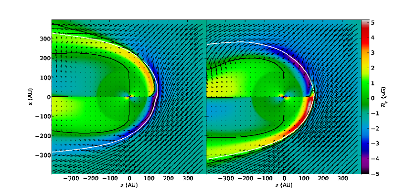
Figure 1: Magnetic field for the heliosphere models used with different solar wind magnetic field polarities, magnetic north positive or de-focusing (left) and magnetic north negative or focusing (right). The colors indicate the strength of the $y$ component of the $B$ field (out of the page) while the arrows indicate the strength and direction of the field projected onto the $x-z$ plane. The white curves indicate the shape of the heliopause, while the black lines separate regions of opposite polarity of $B_{y}$. The different polarities of the field lead to different shapes of the heliosphere because of magnetic reconnection near the heliopause.

Table 1: Boundary Conditions Used in the Heliosphere Models

Quantity	Solar wind	ISM
$n_{p}$ (cm-3)	7.4	0.06
$T$ (K)	$10^{5}$	6,527
$B$ ($\mu$G)	37.5	3.0, 3.6
$B$ direction	$\cdots$	$\ell,b=203\arcdeg,-38\arcdeg$
$v$ (km s-1)	450	26.4
$v$ upwind	$\cdots$	$\ell,b=4\arcdeg,15\arcdeg$

The solar wind in the heliosphere models has a radial velocity at 1 AU of 450 km s^-1 and density of 7.4 cm^-3 and has a Parker spiral magnetic field with strength 37.5 $\mu$G. These boundary conditions are then advected to the inner edge of the 3-D grid at $R=10$ AU. This results in values in the innermost parcel of grid of $v_{r}\approx 454$ km s^-1, $n_{p}\approx 0.07$ cm^-3 and $B_{\phi}\approx 3.3\,\mu$G (near the ecliptic). The temperature evolution in the wind is strongly affected by the interactions between interstellar neutrals and the solar wind ions that produce the pickup ions, and is anisotropic at 10 AU with values ranging from 2800 K to 14,000 K with a mean of 3800 K. These and other boundary conditions in the heliosphere models are summarized in Table 1. It has long been known that the large scale solar magnetic field changes polarity every solar cycle (Howard, 1977, and references therein) and these polarity changes propagate outward with the solar wind. We explore models with both different polarities for the solar wind magnetic field in this work, the focusing polarity that has north pole negative (i.e. north ecliptic pole is south magnetic pole, a.k.a. the $A^{-}$ configuration) and de-focusing that has north pole positive ($A^{+}$ configuration). The reason that the field with north pole negative polarity is focusing for the dust is that, as we discuss further below, the grains are positively charged. Thus $q\vec{v}\times\vec{B}$ points down toward the ecliptic for grains in the north (i.e. above the ecliptic plane) and points up toward the ecliptic for grains in the south. Note that the models we use are steady flow models and so the solar wind magnetic polarity does not evolve. The interstellar medium before the encounter with the heliosphere is assumed to be flowing with speed 26.4 km s^-1 relative to the Sun and have a total proton density of 0.06 cm^-3 and temperature of 6527 K. The neutral H density in the ISM is assumed to be 0.15 cm^-3.

The heliosphere models use a 3-D grid in spherical coordinates (with the polar axis directed towards the longitude of the heliosphere nose), with an inner boundary (radius) at 10 AU and an outer boundary at 1200 AU with 224 zones in the $r$ direction (logarithmically spaced), 144 zones in $\theta$ and 83 in $\phi$. The heliosphere model results include the electron temperature, proton density, magnetic field and velocity over this grid. The grain density grid used is a 3-D Cartesian grid with a spacing of 5 AU in each direction and extending from $-400$ AU to $+400$ AU in each dimension. Note that the computation of the grain trajectories starts farther upwind (900 AU) but the densities are only recorded once the grains enter the density grid. Inside of 10 AU, the dynamical variables are assumed to have their values at the inner edge of the grid.

2.2 Dust Model

We focus on compact olivine-type silicate grains in our models in this paper. Slavin & Frisch (2008) have shown that absorption line data toward $\epsilon$ CMa provide strong evidence that C is not depleted from the gas phase in the LIC, which appears to be the source of the gas flowing into the solar system (Frisch et al., 2011). The depletion pattern of refractory elements in the LIC suggest a grain composition similar to that of olivines, which appear to be widespread in the local ISM (Frisch et al., 2011). Kimura et al. (2003) conclude that C in the local ISM is slightly depleted, but exclude the low H I column density lines of sight in this determination. Thus their method includes mostly gas that is not in the LIC but rather in other clouds. The differences between silicate and carbonaceous grains for the purposes of this paper include the size-to-mass ratio (i.e. the density of the grain material), the charging properties and the grain optical properties (which help determine the value of $\beta$, see below). If future work indicates C depletion in the LIC or the presence of carbonaceous interstellar grains in the heliosphere, a study of such grains would be warranted, though we do not include them in the present study. The solid material density of the grains that we use is 3.3 g cm^-3, as appropriate for olivine silicates, in the results presented in this paper. It has been suggested (e.g., Mathis, 1996) that some or even most interstellar grains may have a porous, or fluffy structure leading to a considerably lower material density. The first fluffy grain models have been ruled out, however based on the excessive amount of infrared emission they would produce (Dwek, 1997). It is currently unclear what fraction of interstellar grains might be fluffy. We intend to explore alternative grain types in future work.

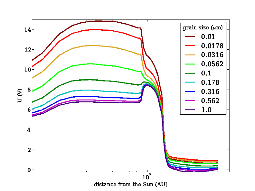
Figure 2: Grain potential (in volts) vs. distance from the Sun (in the upstream direction) for a range of grain sizes. This illustrative calculation was done for grains lying along the $z-$axis (5° from the upstream direction, see text for details about the coordinate system used). The potential varies as a function of the strength of the radiation field (with the solar field going as $1/r^{2}$), but is even more strongly affected in these curves by the plasma temperature. The rise in the potential going outward is thus related to the rise in temperature, which in turn is caused by heating of the solar wind by the pickup ions. The temperature is high in the heliosheath (between 90 and 130 AU), strongly affecting the grain charge. The effects of relative gas-grain velocity are not included in this plot (but are in the trajectory calculations) and tend to increase the potential, especially in the inner heliosphere, by roughly 10%. Some previous modelers of grain trajectories in the heliosphere have used a constant value of 5 V, which is clearly a poor fit to our results with the exception of the largest grains in the inner heliosphere.

The charging properties of interstellar grains are still quite uncertain. In our calculations we use the optical constants and photoelectric yields of Weingartner et al. (2006), making use of their code (kindly provided to us by J. Weingartner), though we have made small modifications to include the effect of gas-grain motion on the charging (using methods described in Guillet et al., 2007). The main sources of charging for interstellar grains in the heliosphere are electron impacts and sticking and photoelectric charging by the FUV radiation field. In regions of hot gas ($T\gtrsim 10^{5}$ K), electrons have enough energy to cause the ejection of secondary electrons, which tends to positively charge the grains. The resultant grain potentials that we find for the upstream direction towards the heliosphere nose are illustrated in Figure 2. The enhanced grain charging in the inner heliosheath, originally discussed by Kimura & Mann (1999), is clearly visible. We find that the grain potential is strongly position and grain size dependent. While the FUV field is dominated by solar radiation in the inner heliosphere, the background interstellar radiation field dominates in the farther regions of the outer heliosphere (see Figure 3). We use the UV radiation field of Gondhalekar et al. (1980) for the background interstellar field (e.g. see the radiation longward of 912 Å in Fig. 1 of Slavin & Frisch, 2008). This field corresponds to a UV flux, averaged over grain photoelectric yield, of 0.74 times that of Draine & Salpeter (1979). For the solar field we use data from the Solar EUV Experiment (SEE) on the NASA TIMED (Thermosphere Ionosphere Mesosphere Energetics and Dynamics, [http://lasp.colorado.edu/see/l3_data_page.html] http://lasp.colorado.edu/see/l3_data_page.html) mission which provides daily EUV/FUV spectra based on solar observations and models and from the SORCE (Solar Radiation & Climate Experiment, [http://lasp.colorado.edu/sorce/index.htm] http://lasp.colorado.edu/sorce/index.htm) mission that provides better visible/near UV data.

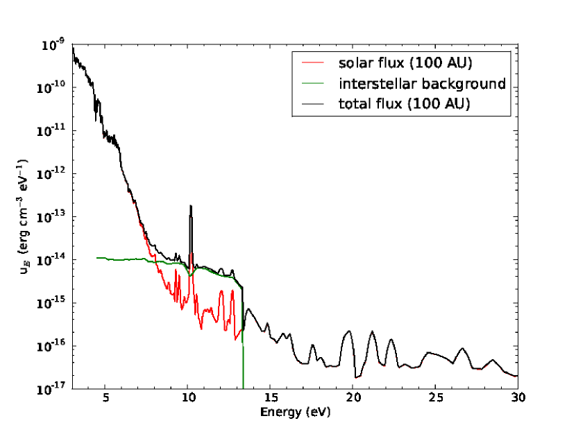
Figure 3: Visible/UV/EUV spectral energy density at 100 AU distance from the Sun. The solar part of the spectrum is based on data from the TIMED-SEE and SORCE missions, while the interstellar background portion is based on the results of Gondhalekar et al. (1980). For charging of silicate grains only the FUV/EUV part of the spectrum above 8 eV (the work function for the grains) is important. The visible and NUV ($\sim 3-6$ eV) parts of the spectrum dominate for heating the grains because of the large flux at those energies. It is clear that the FUV interstellar background radiation field is important at 100 AU, though it becomes less important as the grains penetrate closer to the Sun.

For the inclusion of the effects of radiation pressure and gravity we calculate $\beta$, the ratio of the radiation pressure force to the gravitational force as a function of grain size,

$$\beta=-\frac{F_{r}}{F_{g}}=\frac{R^{2}}{GM_{\odot}m_{\mathrm{gr}}}\frac{1}{c}\int F_{\lambda}\sigma_{\mathrm{gr}}Q_{\mathrm{p}}\,d\lambda,$$ (1)

where $F_{r}$ is the radiation pressure force, $F_{g}$ is the gravitational force, $R$ is the distance from the Sun, $m_{\mathrm{gr}}$ is the grain mass, $F_{\lambda}$ is the flux (erg cm^-2 s^-1 Å^-1) at the distance $R$, $\sigma_{\mathrm{gr}}$ is the physical cross section of the grain and $Q_{\mathrm{p}}$ is the radiation pressure efficiency factor. (For more details see discussions in Gustafson (1994) and Sterken et al. (2012).) Note that $R$ drops out since the flux goes as $1/R^{2}$. This calculation depends on the grain optical properties, through $Q_{\mathrm{p}}$, which in turn depends on the absorption efficiency, $Q_{\mathrm{a}}$, and scattering efficiency, $Q_{\mathrm{s}}$,

$$Q_{\mathrm{p}}=Q_{\mathrm{a}}+(1-g)Q_{\mathrm{s}}$$ (2)

where $g\equiv\langle\cos(\theta)\rangle$ is the scattering asymmetry factor. We calculate the radiation pressure efficiency using results and code from Draine (2003). Using the solar spectrum and our assumed grain density, $\rho_{\mathrm{gr}}=3.3$ g cm^-3, we find that $\beta$ is less than one for all grain sizes. We note that $\beta$ is sensitive to the grain density and composition (Fig. 2 in Kimura et al., 2003), and $\beta$ exceeds 1 (net repulsion of grains) for low density (fluffy) grains. There is some observational evidence for repulsion of grains via radiation pressure, primarily for small grains within 4 AU of the Sun (Fig. 2 in Mann, 2010). Sterken et al. (2012) model variations in $\beta$ and show that $\beta$ is important only within several AU of the Sun (except for downstream where the effects extend farther), in accord with the observations. Given our assumptions, however, the net effect from radiation pressure and gravity on the grains is gravitational focusing though the effect is minor throughout most of the heliosphere. The peak value for $\beta$ is 0.89 at $a_{\mathrm{grain}}\approx 0.2$ µm and so gravity and radiation pressure nearly balance and grains near that size experience little effect from the Sun’s gravity or radiation pressure. As we discuss below and in Slavin et al. (2010), in our models smaller grains are mostly excluded from the inner heliosphere by the solar wind magnetic field, so that uncertainties in $\beta$ do not strongly affect those results. Since the value of $\beta$ decreases as $1/a_{\mathrm{grain}}$ above 0.2 µm, the gravitational effects on the grain trajectories are greatest for the largest grains. These grains also have the smallest charge-to-mass ratios, so gravitational effects play a dominant role in determining their trajectories near the Sun.

3 Grain Trajectory Calculations

We calculate the trajectory of grains by integrating the equation of motion,

$$\ddot{\vec{x}}_{\mathrm{g}}=-(1-\beta)\frac{GM_{\sun}}{|\vec{x}_{\mathrm{g}}|^{3}}\vec{x}_{\mathrm{g}}+\frac{q}{m}((\dot{\vec{x}}_{\mathrm{g}}-\vec{v}_{\mathrm{gas}})\times\vec{B}),$$ (3)

where $\vec{x}_{\mathrm{g}}$ is the grain position relative to the Sun, $q$ is the grain charge, $m$ is the grain mass and $\vec{B}$ is the magnetic field. We also include both the direct drag from gas-grain collisions and plasma drag in our calculations but have found these effects negligible on the scale of the heliosphere. At each point in the integration, the charge is found under the assumption of equilibrium charging based on the radiation field, plasma density, temperature and gas-grain relative velocity at the position of the grain. The equilibrium assumption has been tested and found to be very good. We ignore the quantization of charge in our calculations, which, for small grains, introduces a distribution of possible charge states for any given set of charging conditions (see, e.g. Weingartner & Draine, 2001). In reality the charge distribution will be sampled rapidly by a grain because the charging rates all have short time scales, $\tau\lesssim 10\,\mathrm{s}/a(\mu\mathrm{m})^{2}$. As a result the grain charge will vary with time but the trajectory will tend to hover around that for the equilibrium assumption. Over many grains we expect the net effect of this time varying charge to be small (especially considering the uncertainties in grain charging) and we ignore it in our calculations presented here.

The other quantities that affect the trajectory of a grain, namely the electron and ion density, magnetic field strength and direction, and gas velocity, are taken from the pre-calculated heliosphere models discussed above (see Table 1). The quantities are found via 3-D interpolation of the grid-based model results. We start the grains at a distance of 900 AU from the heliosphere, moving mainly with the gas and with charge appropriate to the conditions. Because grains may be substantially accelerated in the ISM, simply from turbulence present within the cloud, we introduce an initial gyration of the grains around the magnetic field. This initial relative velocity is assumed to be 3 km s^-1 and is perpendicular to the local magnetic field (i.e. pitch angle of $90\arcdeg$) but otherwise randomly directed within that plane. This choice was made to be roughly consistent with recent work on grain acceleration by turbulence by Yan et al. (2004) in which they find that the grains are accelerated to the gas turbulent velocity or more and have large pitch angles. The turbulent velocity of the gas in the LIC is generally found to be $\lesssim 3$ km s^-1 (Redfield & Linsky, 2008). The effect of adding this initial gas-grain motion is not large and mainly serves to smooth out the signature of the initial grid of grain starting points in our final results for grain density presented below.

For each grain size we calculate trajectories of over 10⁶ grains in an initial $1001\times 1001$ grid spaced 1 AU apart. We use the freely available VODE code to carry out the numerical integrations. To calculate the grain space density we set up a grid that is $160\times 160\times 160$ with each cubic voxel 5 AU on a side. After each (fixed) output timestep the count of grains within the voxel in which the grain is located is incremented. With our chosen output timestep we get $\sim 60$ points per voxel (per grain size) in the region where the grain density has yet to be significantly changed from its initial density. To normalize the density to its physical value we need to multiply by the actual assumed density of grains in the ambient ISM. This in turn depends on the gas-to-dust mass ratio, the grain material density (given above) and the initial grain size distribution. Ideally we could go from the observed properties of ISD in the heliosphere to infer the properties of the dust in the ambient ISM, however for completely excluded grains this is obviously not possible and for regions of low density, we are limited by our statistics.

4 Results

4.1 Dust Density Distributions

The primary outputs of our calculations are the 3-D dust density distributions. In Figures 4, 5 and 6 we show slices of the dust density relative to the ambient value for the $z$-$y$, $z$-$x$, and $y$-$x$ planes respectively, comparing results for the de-focusing solar wind magnetic field (SWMF) orientation which has magnetic north (top row) with those for the focusing SWMF polarity (bottom row). These figures are for the smallest grain sizes calculated, $a_{\mathrm{grain}}=0.01$, 0.0178 and 0.0316 $\mu$m. In Figures 7-9 we show the same type of plots for larger grains, $a_{\mathrm{grain}}=0.0562$, 0.1 and 0.178 $\mu$m and in Figures 10-12 for the largest grain sizes calculated, $a_{\mathrm{grain}}=0.316$, 0.562 and 1.0 $\mu$m. The Sun-centered coordinate system used is described above (§2.1). Here the plots are oriented such that the heliosphere is viewed from above for the $z$-$y$ plots, where the upwind direction is to the right and ecliptic longitude increases in negative-y directions. The $z$-$x$ plots show a meridian cut. The $y$-$x$ plots are looking downstream from a viewpoint in the upstream interstellar medium.

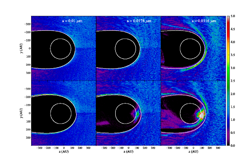
Figure 4: Dust density distributions in slices parallel to the ecliptic plane for 0.01, 0.0178 and 0.0316 µm grains (as labeled). The top row is for the de-focusing SWMF polarity and the bottom row is for the focusing polarity. The color scale indicates the density relative to the ambient interstellar dust density for that grain size. The white curves indicate the termination shock (inner, nearly circular curve) and the heliopause (outer curve). The striping in the image is an artifact of the initial grid of trajectory starting positions.

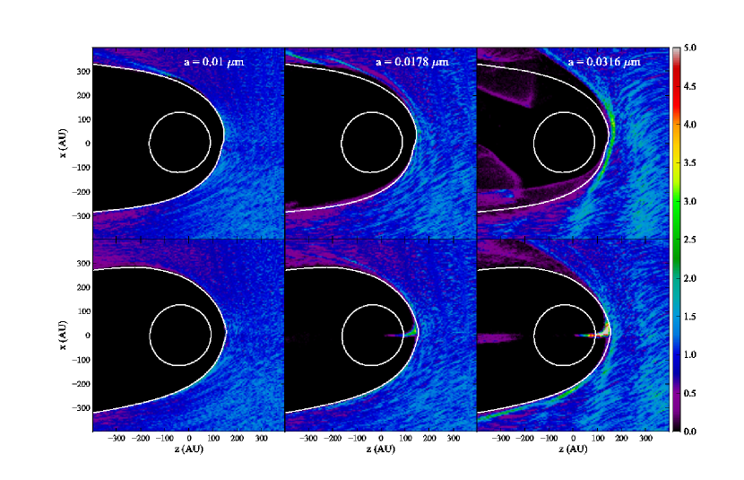
Figure 5: Same as Figure 4 except for slices perpendicular to the ecliptic plane and in the plane of the inflow. Upstream is to the right. As in Figure 4 the top row is for the de-focusing SWMF and the bottom row is for the focusing polarity. Also as in Fig. 4 the inner white curve indicates the location of the termination shock while the outer white curve shows the heliopause location.

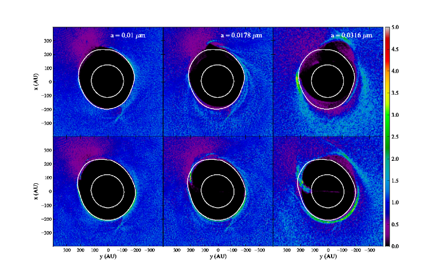
Figure 6: Same as Figure 4 except for slices perpendicular to the ecliptic plane and roughly perpendicular to the interstellar inflow direction. The view orientation is looking downstream (in the $-z$ direction). In this orientation the heliopause appears as the somewhat lopsided white oval outside the more circular termination shock.

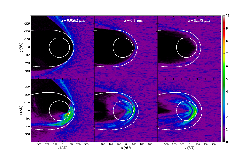
Figure 7: Same as Figure 4 except for 0.0562, 0.1 and 0.178 µm grains (as labeled).

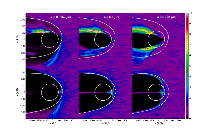
Figure 8: Same as Figure 5 except for 0.0562, 0.1 and 0.178 µm grains (as labeled).

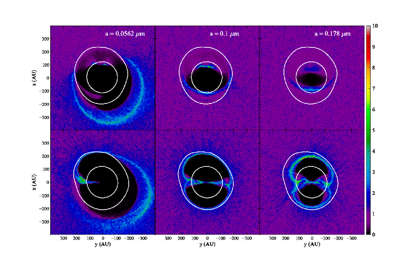
Figure 9: Same as Figure 6 except for 0.0562, 0.1 and 0.178 µm grains (as labeled).

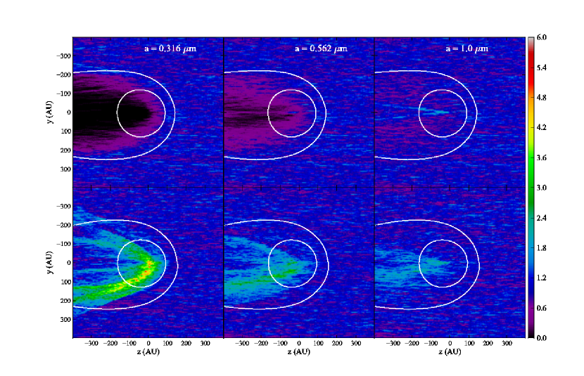
Figure 10: Same as Figure 4 except for 0.316, 0.562 and 1.0 µm grains (as labeled).

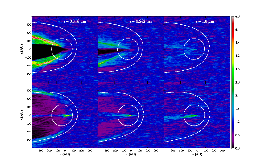
Figure 11: Same as Figure 5 except for 0.316, 0.562 and 1.0 µm grains (as labeled).

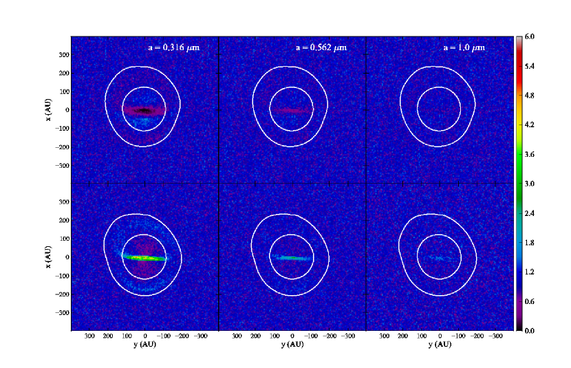
Figure 12: Same as Figure 6 except for 0.316, 0.562 and 1.0 µm grains (as labeled).

An abundance of features are apparent in these model data, but a few stand out immediately. First, it is clear that for the de-focusing SWMF polarity only fairly large grains, $a_{\mathrm{gr}}\gtrsim 0.3$ µm, can reach Earth’s orbit, though grains as small as 0.1 µm can penetrate the termination shock. Thus it is hard to reconcile this model with the observed size distribution, which includes grains as small as $\sim 0.05$ µm. For the focusing polarity field, again grains as small as 0.1 µm can penetrate the termination shock, but in this case the focusing effects of the SWMF allows such grains to reach all the way to the Sun, as they are concentrated in the ecliptic plane. Indeed even grains as small as 0.02 µm can reach the Sun for the focusing polarity. These strong differences in the distributions of dust grains of a given size between the different magnetic polarities persists, even up to 1 µm grains, though for larger grains the focusing/de-focusing effects of the SWMF are relatively small and mitigated by the effects of gravitational focusing by the Sun. Even for the largest grains, $a=1$ µm, the dust focusing tail shows some solar cycle dependence (e.g. Figures 10–12). For both SWMF polarities, the dust trajectories and thus dust density distributions are quite sensitive to grain size. This is because the gyroradii of the grains range from $<1$ AU for 0.01 µm grains to $\sim 10^{5}$ AU for 1 µm grains at the heliopause.

In the dust density figures it is clear that the smallest grains are effectively completely excluded from the inner heliosheath, being diverted along with the interstellar plasma around the heliopause. At larger grain sizes, more penetration of the heliopause and the effects of the larger gyroradii can be seen. As an example, in Fig. 5 in the upper right panel ($a=0.0316$ µm), the low densities for large $x$ values above the heliopause show how grains that have been diverted do not follow the heliopause, but gain a substantial $+x$ velocity that carries them away from the heliosphere. The regions with significant dust density inside the heliopause in this panel are from scattering of grains in from the flanks of the heliopause (because their gyroradii are large enough to allow them to cross the heliopause). The enhancement in grain density in the region just upwind of the heliopause in the $z$-$y$ plot for this same grain size is also caused by the decoupling. The effects of decoupling of the grains from the gas become much more pronounced for larger grain sizes. For 0.0562 µm grains the effects of scattering off the heliopause are clear in Figs. 7-9. In the $z$ slices in particular, it can be seen that the grains, which have a small initial $-x$ velocity (recall that the upwind direction is $\sim 5\arcdeg$ above the $+z$ axis) are deflected by about 200 AU over the $\sim 150$ AU distance since encountering the heliopause. We note that this grain size is peculiar in our results because for both the de-focusing and focusing SWMF models we find a zero density for the voxels near the Sun, although for the focusing SWMF smaller grains (0.0178, 0.0316 µm) do produce non-zero density. This result, which we discuss more below, appears to be caused by the fact that grains of this size have gyroradii at the location of encountering the heliopause, that are roughly the same size as the heliopause. They thus decouple substantially from the gas, but are strongly diverted from their inflow paths.

Smaller grains, while more tightly coupled to the plasma (via the magnetic field), can scatter and leak into the heliosphere wherein they may be focused towards the ecliptic for the focusing SWMF. Larger grains, while even more decoupled from the plasma, are less diverted from their paths and, again for the focusing SWMF, have an enhanced dust density near the Sun. As the grain size increase, grains in the range of $\sim 0.05-0.2$ µm (Figs. 7–12) show increasing degrees of penetration of the heliopause and are focused either near the ecliptic poles, for the de-focusing SWMF, or in the ecliptic, for the focusing SWMF. The 3-D grain density distribution for 0.178µm grains is illustrated in Figure 13, which shows a rendering of the 3-D surfaces corresponding to dust density enhancements (relative to the interstellar density) of 2, 2.75, 3.5, 4.25 and 5. Going to the largest grain sizes (Figs. 10-12) the grains are less and less affected by the heliopause and at the largest size, 1.0 µm, are primarily affected by the gravitational focusing by the Sun.

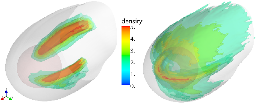
Figure 13: Dust density enhancement for 0.178 µm grains in the heliosphere rendered as the 3-D surfaces corresponding to factors of 2, 2.75, 3.5, 4.25 and 5 over the ambient density. The de-focusing SWMF case is shown on the left and the focusing SWMF polarity case is shown on the right. It can be seen that the focusing SWMF leads to enhanced density in a crescent shaped region near the ecliptic plane while the de-focusing field leads to concentration of the dust at the north and south ecliptic poles. These plumes of dust in the constant polarity models, should blend into each other in the true heliosphere with its time-variable SWMF polarity. Note: the interstellar inflow comes from the lower left and flows toward the upper right.

The individual grain trajectories can be quite complex, especially for the intermediate grain sizes, $\sim 0.05-0.3$ µm, for which the grains are significantly diverted from their original path but have large enough gyroradii to penetrate to the inner heliosphere. The scattering of the grains inside the heliosphere is clear as even grains that start out on similar trajectories diverge strongly from each other. This scattering is primarily caused by the fact that the gyroradii are as large or larger than a typical length scale for variation in the magnetic field direction so the field sampled by different grains on their trajectories is substantially different and becomes more so as they propagate closer to the heliopause and inner heliosphere. The differences in trajectories are also amplified by the increase in magnetic field strength caused by compression in the heliosheath.

4.2 Grain Size Distribution

One of the most important reasons for calculating grain trajectories through the heliosphere starting from the undisturbed ISM is to allow us to infer the initial interstellar grain size distribution given the size distribution observed by the Ulysses and Galileo spacecrafts. With accurate 3-D heliosphere models and grain trajectory calculations one could, in principle, infer from the observations the interstellar size distribution, though of course grain sizes that are either completely excluded from the inner heliosphere or not observable because of instrumental limitations cannot be constrained by this method. In this study we have made progress toward this goal by employing accurate, though non-evolving, heliosphere models. As we discuss further below, however, the lack of solar cycle evolution of the heliosphere, in particular the SWMF, during the time the grains traverse the inner heliosphere limits the applicability of our results. Assuming either a focusing or de-focusing SWMF during an entire grain trajectory effectively exaggerates the focusing or de-focusing the grains will experience. We expect that the truth will lie in between these extreme cases. The detailed behavior of the grains with small to moderate gyroradii as the SWMF evolves is unclear at present especially considering the complex magnetic topology caused by the evolution and propagation of the heliospheric current sheets (Nerney et al., 1995). Despite these limitations, we find below that comparisons between our models and the in situ data provide valuable insights into the properties of the grains and their interaction with the heliosphere.

Our calculations do not assume any particular size distribution (being carried out independently for each grain size) since the grains are not assumed to interact significantly with each other. This assumption should be excellent over the length scales relevant for the heliosphere, though in interstellar shocks (with length scales hundreds of thousands of times longer), grain-grain collisions are a major source of dust destruction (Jones et al., 1994). The output of our calculations provide an unbiased result for each grain size, since the dust density at each point in space is calculated relative to its value in the ISM prior to interaction with the heliosphere.

Comparisons between the models and the in situ observations are not useful for the smallest grains or for regions of the model that are infrequently populated with grains. For the smallest grains, below the detection threshold of the Ulysses and Galileo dust detectors ($m\approx 7\times 10^{-16}$ g or $a\approx 0.04$ µm for our assumed grain density), we obviously have no information on their abundance in the heliosphere. Use of our theoretical data is also limited by our statistics: if we have no counts in a voxel, this simply gives us an upper limit on our predicted dust density relative to the initial interstellar dust density for grains in that size range. In the calculations that we present in this paper, we expect, on average, $\sim 62$ counts per voxel (5 AU in each dimension) if the dust density were undisturbed from its value in the ambient ISM. Thus if the dust density for a particular grain size is reduced by a factor of $\gtrsim 62$ then we are likely to get no counts in the voxel and we are not sensitive to how large the reduction in dust density is above that threshold.

Although our calculations use a regular grid of starting points for the trajectories, they are, in some sense, similar to Monte Carlo calculations. Each individual trajectory is quite sensitive to its initial conditions, so the starting positions, which have no a priori justification other than being sufficiently far upstream of the heliosphere, could be considered to be random choices. A slight shifting of the starting grid would lead to considerably different individual trajectories, though the dust density results would be essentially unchanged. In addition, as mentioned above, the initial gyrovelocity for each grain has a random direction other than that is in the plane perpendicular to the magnetic field (i.e. 90° pitch angle). This small addition of randomness to the initial velocities is sufficient to remove most of the identifiable signature of the initial grid in the final dust density results. Thus we can treat the dust density results in a statistical manner and assume the uncertainty in the “true” number of counts we should get for each voxel is consistent with Poisson statistics. As shown by Gehrels (1986), for small numbers of counts the usual $\sqrt{N}$ approximation is not a good approximation for the confidence limits and we use instead his results to determine the statistical 1-$\sigma$ error bars. The 1-$\sigma$ upper limits are $1+N+\sqrt{N+\frac{3}{4}}$ and lower limits are $N\left(1-\frac{1}{9N}-\frac{1}{3\sqrt{N}}\right)^{3}$. Thus for a voxel in with no counts, the upper limit is $1+\sqrt{\frac{3}{4}}$.

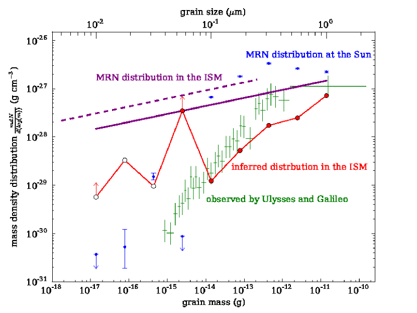
Figure 14: Size distribution of interstellar grains in the ISM and the heliosphere (plotted as mass density distributions). In green are the Ulysses and Galileo data where the bin widths are set so as to get the same total number of counts per bin (see Frisch et al., 2009). Plotted in purple are the standard Mathis et al. (1977) size distribution which cuts off at $a_{\mathrm{gr}}=0.25$ µm (dashed) and the same power law but extended to 1 µm. Those size distributions are both normalized so as to produce a gas-to-dust mass ratio of 150. In blue is plotted the size distribution that would be observed near the Sun if the interstellar size distribution were the extended MRN and the focusing SWMF polarity model applied. The error bars here are statistical. The red line shows the inferred interstellar grain size distribution given the observed size distribution and the modeled grain transport (again for the focusing SWMF polarity). The empty circles at the small grain size end are based on an extrapolation of the observed grain size distribution below the detection threshold.

To scale the results of our models to actual densities in the ISM or heliosphere we need to assume an initial grain size distribution including the scaling relative to the gas density. Differences between the initial grain distribution at “infinity” and the observed in situ dust distribution should then be explained in principle by grain propagation models. In Figure 14 we show the data from Frisch et al. (2009, and references therein) for Ulysses and Galileo dust detection along with models and inferred grain size distributions. Here, rather than the grain size distribution, $\frac{dn}{da}$, we plot the grain mass per logarithmic mass bin as was done in Frisch et al. (1999) and Frisch et al. (2009). Plotted this way, it is apparent that most of the mass is in grains on the large end of the scale. In the figure, we plot the standard MRN power-law distribution for grain sizes (Mathis et al., 1977, dashed, purple curve) which extends from 0.005 µm to 0.25 µm with the normalization set by the assumption of an interstellar density of $n_{\mathrm{H}}=0.22$ cm^-3 and a gas-to-dust mass ratio of 150. The H density and gas-to-dust ratio are taken from the LIC photoionization models of Slavin & Frisch (2008), which are successful in that they predict interstellar boundary conditions for the heliosphere that are consistent with local ISM parameters derived from heliosphere models. Since the upper size cutoff for the standard MRN size distribution is well below the size of the largest grains observed (for silicate grains; graphite grains sizes up to 1 µm are allowed), we also plot an MRN-type size distribution but with higher lower and upper size limits ($0.01-1.0$ µm), and using the same $n_{\mathrm{H}}$ and dust-to-gas ratio for normalization, that we refer to as a “shifted MRN” size distribution. We note that more recent detailed ISM grain models such as Zubko et al. (2004) have grain size distributions that differ substantially from a simple power-law and in some cases extend significantly above the 0.25 µm cutoff of the MRN model. However, no proposed ISM grain model has a size distribution similar to that observed in the heliosphere (Draine, 2009), because such a size distribution is inconsistent with observed extinction curves. We note, however, that the extinction curves that such grain models aim to match are derived from observations over kiloparsec long lines of sight. This implies that either the size distribution in the LIC is very atypical of the ISM or it has been substantially distorted by the transit of the grains through the heliosphere. Our results provide insights into the effects of those distortions.

If we assume that the shifted MRN distribution, represents the grain size distribution in the undisturbed ISM, then, using the focusing SWMF polarity heliosphere model, we find that we would expect the detections shown as the blue points in Figure 14. For these points we use the density results for the voxels consistent with the orbit of Ulysses, including ranges in $x$, $y$ and $z$ of $-3$ to $+3$ AU, $-1.3$ to $+5.4$ AU and $-2.1$ to $+2.1$ AU respectively (using the coordinate system described in §2.1 above). The points are generally well above the actual detections except for the point at 0.0562 µm, for which no counts are found in the model for the region close to the Sun (see discussion below). This suggests that the focusing model provides too much focusing (at least for the assumed size distribution), as would be expected if the grains experienced a de-focusing phase as well as focusing during their transit of the heliosphere. If instead we use the actual observations (interpolated to get the grain densities at the calculated grain sizes) then we can infer the size distribution in the interstellar medium by using the model enhancement/depletion of grains caused interaction with the heliosphere. We have done that, using spline interpolation on the data, with the results plotted as the red points in the figure. These points are correspondingly well below the shifted MRN model line (again with the exception of the 0.0562 µm grains). In going from the observed points to the size distribution in the undisturbed ISM we divide by the enhancement factor, i.e. ratio of dust density for grains of a given size to that in the undisturbed ISM. Therefore a larger enhancement leads to a lower value inferred for the ISM. Thus the model with the focusing SWMF polarity appears to over-predict the focusing and predicts a very small dust-to-gas ratio in the LIC.

At the low end of the size distribution we have done a linear (in the log, i.e. powerlaw) extrapolation of the data down from the $\sim 0.1$ µm detection threshold of Ulysses to 0.01 µm to explore the implications for the grain size distribution. If the grain size distribution near the Sun really does extend in this way to smaller sizes, then the model results imply a flattening of the size distribution in the ISM for for these small grain sizes. Since we there is no data on interstellar grains of those sizes in the heliosphere, this result (which also only applies for the focusing-only SWMF) is purely speculative at this point.

If we instead interpret the dust measurements using the de-focusing SWMF polarity model the results are starkly different. Since all but the three largest grain sizes modeled (0.316, 0.562 and 1.0 µm) produce no counts for the voxels near the Sun, the inferred distribution of grains in the ISM has, except for grain sizes $\geq 0.316$ µm, very high lower limits that generally exceed the extended MRN distribution. Such a high density of dust would demand a small gas-to-dust mass ratio, $R_{g/d}<38$, and would conflict with limits on total cosmic abundances for the elements that make up the dust. On the other hand the results for the focusing SWMF polarity model (discussed above) implies a rather small dust density and thus a high gas-to-dust ratio, $R_{g/d}\sim 820$ (ignoring the 0.0562 µm grain size). This would indicate a high degree of dust destruction in the ISM and only a small mass of heavy elements tied up in the dust. This again conflicts with observations, in particular those that indicate significant gas phase depletion of several elements, e.g. Fe, Mg and Si, from the gas phase (Slavin & Frisch, 2008).

The fact that neither the focusing SWMF nor de-focusing SWMF models can be comfortably accommodated with our information on gas phase elemental abundances in the LIC points to the limitations of constant polarity models for the SWMF. This is not surprising since the grains require $\sim 20$ years to travel between the termination shock and inner heliosphere. The fact that the predictions of our two heliosphere models lead to bracketing of the likely possibilities for the inferred gas-to-dust ratio and grain size distribution suggests that grain trajectory modeling needs to include the time variation of the solar wind, and its magnetic field polarity in particular, over the solar cycle. The strong dependence of the grain density on the SWMF polarity shows that the recovery of the mass distribution of interstellar dust from in situ measurements requires a complete understanding of the effect of the solar cycle on the global heliosphere, and grain trajectory models that incorporate interactions with the 3-D global heliosphere.

We note that the grains with the particular size of 0.0562 µm are predicted to have very low density (zero counts calculated) near the Sun for both heliosphere models, though for the focusing SWMF model a substantial amount of dust penetrates the heliopause. As discussed in §4 above, this appears to be caused by the size of the gyroradius for grains of this size, which is large enough that the grains decouple from the gas enough to penetrate the heliopause and termination shock, but small enough that their path is substantially diverted from its initial direction. We expect that additional perturbations to the initial conditions for the grains and especially spatial and temporal variations in the solar wind will wash out this feature leading to a relatively featureless grain size distribution such as is observed.

The heliosphere models that we use in this paper are consistent with all the information available up until recently on the ISM and the heliosphere. This includes the speed of the inflowing ISM and the orientation of the interstellar magnetic field required to produce the asymmetry in the shape of the termination shock as revealed by the location of the Voyager 1 and 2 crossings. Recent data from IBEX (Möbius et al., 2012) indicate that the speed of the interstellar inflow is about 12% less than previously determined, $\sim 23$ km s^-1 rather than 26.4 km s^-1. This lower velocity appears to to rule out a bow shock ahead of the heliosphere (McComas et al., 2012). If this result holds up, then other parameters of the heliosphere models, e.g. interstellar magnetic field strength, will likely require some small adjustments as well. We do not expect this to make any difference regarding the fundamental conclusions of this paper, especially since the models that we have used already do not have a shock transition between the ISM and the outer heliosheath.

5 Conclusions

We have presented the first simulations of interstellar grain propagation through the heliosphere that have incorporated a realistic 3-D global heliosphere model that accommodates recently gained knowledge on the shape and size of the heliosphere, including the asymmetries due to the large angle between the interstellar gas flow and ISMF direction. While our understanding of the heliosphere continues to improve, the heliosphere models used in this study capture the essential characteristics of its shape and the characteristics that affect distribution of ISD in the heliosphere (except for its time variability during grain propagation).

Our models include detailed calculations of the grain charging based on a standard interstellar grain model, using olivine silicates with density 3.3 gr cm^-3, and including a realistic solar radiation field. The calculations follow the grain trajectories that originate in the undisturbed interstellar medium well outside of the heliosphere. Our results indicate that inferences on the grain size distribution and abundance in the interstellar medium surrounding the heliosphere depend sensitively on the heliosphere model and in particular on the polarity of the solar wind magnetic field. For a focusing polarity of the field, grains over a wide size range can penetrate the heliopause and are focused in the ecliptic. For de-focusing polarity, only the larger grains we studied, $\gtrsim 0.3$ µm, are found to create non-zero density at the Sun. For either SWMF polarity, the largest grains ($\sim 1$ µm) have enhanced dust density relative to that in the ISM, because of gravitational focusing, which helps to explain the larger than expected observed density of large grains in the inner heliosphere near the Sun.

Grains in the size range near 0.2 µm are diverted into dust plumes along the flanks of the heliosphere inside of the termination shock, with the plumes located in the polar regions for the de-focusing polarity model and in the ecliptic region for the focusing polarity model. In the true time-variable heliosphere, these dust grains will sample both polarities of the SWMF and the different magnetic morphologies and solar wind conditions that will exist over the course of the solar cycle. We speculate that this may lead to these dust density enhancements being smeared into some shape in between these extremes, perhaps an asymmetric dust shell inside of the termination shock but somewhat upstream of the Sun. Such a feature has the potential to create an unaccounted for contribution to the infrared and microwave sky background. This possibility requires further investigation.

The total dust density inferred for the ISM, using our models, is either too small, for the focusing polarity, or too large, for the de-focusing polarity to be consistent with the gas phase abundances inferred from absorption line data (e.g., Slavin & Frisch, 2008). This points to the need to use heliosphere models that include the time dependence of the solar wind magnetic field over the course of a solar cycle in grain trajectory calculations. Our calculations, by using a single polarity for the SWMF over the decades long course of a grain trajectory, effectively bracket the possible outcomes for the grain density inside the heliosphere. With future calculations that include the time evolution of the SWMF we hope to narrow the range of predicted grain densities, leading to a robust inference on the interstellar grain size distribution from in situ observations of interstellar dust in the heliosphere.

Appendix A Individual Grain Trajectories

Examination of trajectory groups in the model calculations shows the complexity of individual trajectories. In Figure 15 we show a group of 16 trajectories for 0.178 µm grains that result in relatively close passage to the Sun to illustrate more clearly the way in which grains are scattered in the inner heliosphere. Gravity and radiation pressure do not have a strong influence on these trajectories though for somewhat larger grains, gravity does play an important role for grains passing near the Sun. Some trajectories are dominated by a single scattering due to the Lorentz force, while others experience several scatterings. The small initial gyrovelocity given to the grains (due to interstellar turbulence) acts to create a stochastic element to the trajectories which is enhanced by their subsequent interactions with heliosphere.

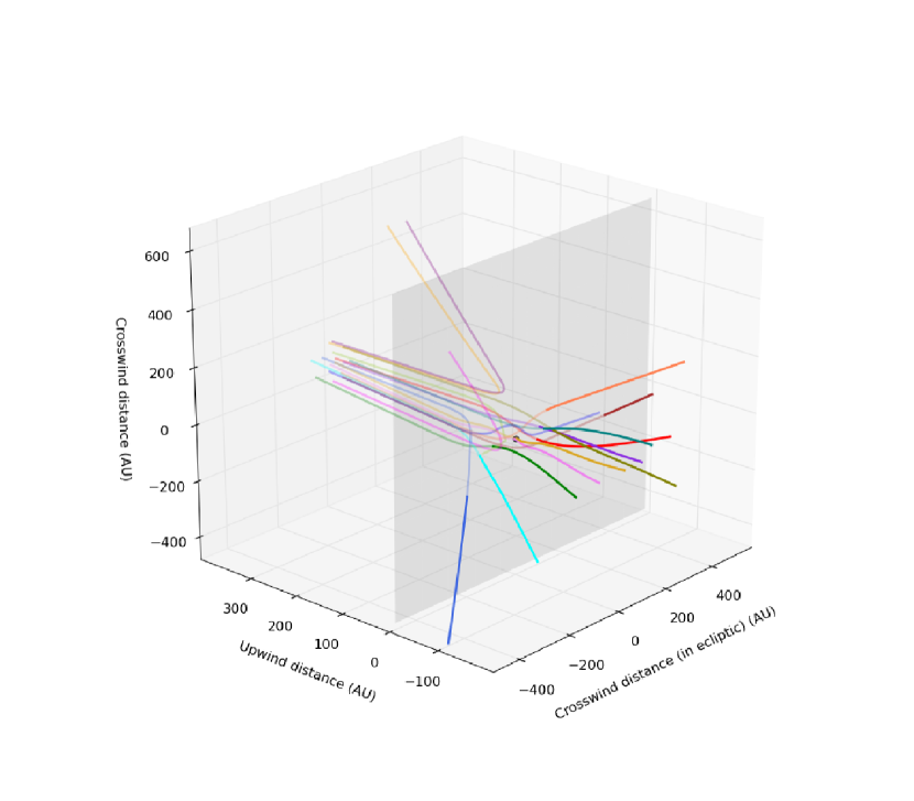
Figure 15: Trajectories for 0.178 µm grains for focusing polarity. Included in the plot are just the parts of the trajectories with $z$ between $-200$ and $+400$ AU. The color coding was done as a way to help trace the trajectories. Also the trajectories are transparent when they are upwind and once they cross the $z=0$ plane, indicated by the transparent plane, they are made opaque. The Sun’s location is indicated by a circle. Note the strong level of scattering experienced by some grains, while for others their trajectories are relatively straight. These trajectories are a small subset of the more than $10^{6}$ trajectories calculated to make the dust density plots.

References

- Altobelli et al. (2007) Altobelli, N., Dikarev, V., Kempf, S., Srama, R., Helfert, S., Moragas-Klostermeyer, G., Roy, M., & Grün, E. 2007, Journal of Geophysical Research (Space Physics), 112, 7105
- Czechowski & Mann (2003) Czechowski, A. & Mann, I. 2003, Journal of Geophysical Research (Space Physics), 108, 8038
- Draine (2003) Draine, B. T. 2003, ApJ, 598, 1017
- Draine (2009) —. 2009, Space Sci. Rev., 143, 333
- Draine & Salpeter (1979) Draine, B. T. & Salpeter, E. E. 1979, ApJ, 231, 77
- Dwek (1997) Dwek, E. 1997, ApJ, 484, 779
- Frisch et al. (2009) Frisch, P. C., Bzowski, M., Grün, E., Izmodenov, V., Krüger, H., Linsky, J. L., McComas, D. J., Möbius, E., Redfield, S., Schwadron, N., Shelton, R., Slavin, J. D., & Wood, B. E. 2009, Space Sci. Rev., 146, 235
- Frisch et al. (1999) Frisch, P. C., Dorschner, J. M., Geiss, J., Greenberg, J. M., Grün, E., Landgraf, M., Hoppe, P., Jones, A. P., Krätschmer, W., Linde, T. J., Morfill, G. E., Reach, W., Slavin, J. D., Svestka, J., Witt, A. N., & Zank, G. P. 1999, ApJ, 525, 492
- Frisch et al. (2011) Frisch, P. C., Redfield, S., & Slavin, J. D. 2011, ARA&A, 49, 237
- Gehrels (1986) Gehrels, N. 1986, ApJ, 303, 336
- Gloeckler & Fisk (2007) Gloeckler, G. & Fisk, L. 2007, Space Sci. Rev., 27, 489
- Gondhalekar et al. (1980) Gondhalekar, P. M., Phillips, A. P., & Wilson, R. 1980, A&A, 85, 272
- Grogan et al. (1996) Grogan, K., Dermott, S. F., & Gustafson, B. A. S. 1996, ApJ, 472, 812
- Grün et al. (1994) Grün, E., Gustafson, B., Mann, I., Baguhl, M., Morfill, G. E., Staubach, P., Taylor, A., & Zook, H. A. 1994, A&A, 286, 915
- Grün & Svestka (1996) Grün, E. & Svestka, J. 1996, Space Sci. Rev., 78, 347
- Guillet et al. (2007) Guillet, V., Pineau Des Forêts, G., & Jones, A. P. 2007, A&A, 476, 263
- Gustafson (1994) Gustafson, B. A. S. 1994, Annual Review of Earth and Planetary Sciences, 22, 553
- Heerikhuisen et al. (2006) Heerikhuisen, J., Florinski, V., & Zank, G. P. 2006, Journal of Geophysical Research (Space Physics), 111, 6110
- Heerikhuisen et al. (2008) Heerikhuisen, J., Pogorelov, N. V., Florinski, V., Zank, G. P., & le Roux, J. A. 2008, ApJ, 682, 679
- Howard (1977) Howard, R. 1977, Annual Review of Astronomy and Astrophysics, 15, 153
- Jones et al. (1994) Jones, A. P., Tielens, A. G. G. M., Hollenbach, D. J., & McKee, C. F. 1994, ApJ, 433, 797
- Kimura & Mann (1999) Kimura, H. & Mann, I. 1999, Earth, Planets, and Space, 51, 1223
- Kimura et al. (2003) Kimura, H., Mann, I., & Jessberger, E. K. 2003, ApJ, 582, 846
- Kimura et al. (2003) Kimura, H., Mann, I., & Jessberger, E. K. 2003, ApJ, 583, 314
- Krüger et al. (2010) Krüger, H., Dikarev, V., Anweiler, B., Dermott, S. F., Graps, A. L., Grün, E., Gustafson, B. A., Hamilton, D. P., Hanner, M. S., Horányi, M., Kissel, J., Linkert, D., Linkert, G., Mann, I., McDonnell, J. A. M., Morfill, G. E., Polanskey, C., Schwehm, G., & Srama, R. 2010, Planet. Space Sci., 58, 951
- Lallement et al. (2005) Lallement, R., Quémerais, E., Bertaux, J. L., Ferron, S., Koutroumpa, D., & Pellinen, R. 2005, Science, 307, 1447
- Lallement et al. (2010) Lallement, R., Quémerais, E., Koutroumpa, D., Bertaux, J., Ferron, S., Schmidt, W., & Lamy, P. 2010, Twelfth International Solar Wind Conference, 1216, 555
- Landgraf (2000) Landgraf, M. 2000, J. Geophys. Res., 105, 10303
- Landgraf et al. (2000) Landgraf, M., Baggaley, W. J., Grün, E., Krüger, H., & Linkert, G. 2000, J. Geophys. Res., 105, 10343
- Landgraf et al. (2003) Landgraf, M., Krüger, H., Altobelli, N., & Grün, E. 2003, Journal of Geophysical Research (Space Physics), 108, 8030
- Mann (2010) Mann, I. 2010, ARA&A, 48, 173
- Mathis (1996) Mathis, J. S. 1996, ApJ, 472, 643
- Mathis et al. (1977) Mathis, J. S., Rumpl, W., & Nordsieck, K. H. 1977, ApJ, 217, 425
- McComas et al. (2012) McComas, D. J., Alexashov, D., Bzowski, M., Fahr, H., Heerikhuisen, J., Izmodenov, V., Lee, M. A., Möbius, E., Pogorelov, N., Schwadron, N. A., & Zank, G. P. 2012, Science, 336, 1291
- McComas et al. (2009) McComas, D. J., Allegrini, F., Bochsler, P., Bzowski, M., Christian, E. R., Crew, G. B., DeMajistre, R., Fahr, H., Fichtner, H., Frisch, P. C., Funsten, H. O., Fuselier, S. A., Gloeckler, G., Gruntman, M., Heerikhuisen, J., Izmodenov, V., Janzen, P., Knappenberger, P., Krimigis, S., Kucharek, H., Lee, M., Livadiotis, G., Livi, S., MacDowall, R. J., Mitchell, D., Möbius, E., Moore, T., Pogorelov, N. V., Reisenfeld, D., Roelof, E., Saul, L., Schwadron, N. A., Valek, P. W., Vanderspek, R., Wurz, P., & Zank, G. P. 2009, Science, 326, 959
- Möbius et al. (2012) Möbius, E., Boschler, M., Bzowski, M., Heirtzler, D., Kubiak, M. A., Kucharek, H., Lee, M. A., Leonard, T., Schwadron, N. A., Wu, X., Fuselier, S. A., Crew, G., McComas, D. J., Petersen, L., Saul, L., Valovcin, D., Vanderspek, R., & Wurz, P. 2012, ApJ, 198, 11
- Morfill & Grün (1979) Morfill, G. E. & Grün, E. 1979, Planet. Space Sci., 27, 1283
- Nerney et al. (1995) Nerney, S., Suess, S. T., & Schmahl, E. J. 1995, J. Geophys. Res., 100, 3463
- Pagani et al. (2010) Pagani, L., Steinacker, J., Bacmann, A., Stutz, A., & Henning, T. 2010, Science, 329, 1622
- Pogorelov et al. (2008) Pogorelov, N. V., Heerikhuisen, J., & Zank, G. P. 2008, ApJ, 675, L41
- Redfield & Linsky (2008) Redfield, S. & Linsky, J. L. 2008, ApJ, 673, 283
- Reisenfeld et al. (2012) Reisenfeld, D. B., Allegrini, F., Bzowski, M., Crew, G. B., DeMajistre, R., Frisch, P., Funsten, H. O., Fuselier, S. A., Janzen, P. H., Kubiak, M. A., Kucharek, H., McComas, D. J., Roelof, E., & Schwadron, N. A. 2012, ApJ, 747, 110
- Schwadron et al. (2011) Schwadron, N. A., Allegrini, F., Bzowski, M., Christian, E. R., Crew, G. B., Dayeh, M., DeMajistre, R., Frisch, P., Funsten, H. O., Fuselier, S. A., Goodrich, K., Gruntman, M., Janzen, P., Kucharek, H., Livadiotis, G., McComas, D. J., Moebius, E., Prested, C., Reisenfeld, D., Reno, M., Roelof, E., Siegel, J., & Vanderspek, R. 2011, ApJ, 731, 56
- Schwadron et al. (2009) Schwadron, N. A., Bzowski, M., Crew, G. B., Gruntman, M., Fahr, H., Fichtner, H., Frisch, P. C., Funsten, H. O., Fuselier, S., Heerikhuisen, J., Izmodenov, V., Kucharek, H., Lee, M., Livadiotis, G., McComas, D. J., Moebius, E., Moore, T., Mukherjee, J., Pogorelov, N. V., Prested, C., Reisenfeld, D., Roelof, E., & Zank, G. P. 2009, Science, 326, 966
- Slavin & Frisch (2008) Slavin, J. D. & Frisch, P. C. 2008, A&A, 491, 53
- Slavin et al. (2010) Slavin, J. D., Frisch, P. C., Heerikhuisen, J., Pogorelov, N. V., Mueller, H.-R., Reach, W. T., Zank, G. P., Dasgupta, B., & Avinash, K. 2010, Twelfth International Solar Wind Conference, 1216, 497
- Sterken et al. (2012) Sterken, V. J., Altobelli, N., Kempf, S., Schwehm, G., Srama, R., & Grün, E. 2012, A&A, 538, A102
- Stone et al. (2008) Stone, E. C., Cummings, A. C., McDonald, F. B., Heikkila, B. C., Lal, N., & Webber, W. R. 2008, Nature, 454, 71
- Weingartner & Draine (2001) Weingartner, J. C. & Draine, B. T. 2001, ApJ, 548, 296
- Weingartner et al. (2006) Weingartner, J. C., Draine, B. T., & Barr, D. K. 2006, ApJ, 645, 1188
- Witte (2004) Witte, M. 2004, A&A, 426, 835
- Yan et al. (2004) Yan, H., Lazarian, A., & Draine, B. T. 2004, ApJ, 616, 895
- Zank (1999) Zank, G. P. 1999, Space Sci. Rev., 89, 413
- Zubko et al. (2004) Zubko, V., Dwek, E., & Arendt, R. G. 2004, ApJS, 152, 211