Anomalous phonon behavior of carbon nanotubes: First-order influence of external load

Abstract

External loads typically have an indirect influence on phonon curves, i.e., they influence the phonon curves by changing the state about which linearization is performed. In this paper, we show that in nanotubes, the axial load has a direct first-order influence on the long-wavelength behavior of the transverse acoustic (TA) mode. In particular, when the tube is force-free, the TA mode frequencies vary quadratically with wave number and have curvature (second derivative) proportional to the square-root of the nanotube’s bending stiffness. When the tube has non-zero external force, the TA mode frequencies vary linearly with wave number and have slope proportional to the square-root of the axial force. Therefore, the TA phonon curves—and associated transport properties—are not material properties but rather can be directly tuned by external loads. In addition, we show that the out-of-plane shear deformation does not contribute to this mode and the unusual properties of the TA mode are exclusively due to bending. Our calculations consist of 3 parts: First, we use a linear chain of atoms as an illustrative example that can be solved in close-form; second, we use our recently developed symmetry-adapted phonon analysis method to present direct numerical evidence; and finally, we present a simple mechanical model that captures the essential physics of the geometric nonlinearity in slender nanotubes that couples the axial load directly to the phonon curves. We also compute the density of states and show the significant effect of the external load.

1 Introduction

The low-dimensionality of nanotubes causes unusual features in the phonon curves due to geometric effects. In this paper, we examine particularly the transverse acoustic (TA) phonon mode and its slope and curvature (second derivative) in the long wavelength limit.

Previous works have reported four acoustic modes of vibration for SWNT. There is consensus that two of the modes (longitudinal and twisting modes) have linear dispersion in the long wavelength limit. However, there has been discussion about the form of the other two TA modes which are doubly degenerate. E.g., several papers [1, 2, 3, 4, 5, 6, 7, 8, 9] report linear dispersion for the TA modes. These authors do not analytically show that the TA modes should be linear, but argue that nanotubes do not have modes analogous to the out-of-plane “bending” mode of graphene, and thus, nanotubes must have linear long wavelength acoustic dispersion behavior. Among these works, two recent papers [7, 9] state that quadratic dependence is found in some other papers, but argue that this may be attributed to numerical errors.

In contrast, more recent papers [10, 11, 12, 13, 14, 15, 16, 17] report a quadratic dependence of frequency on the wave number. The results presented in these papers are obtained by applying lattice dynamics methods to either tight-binding, ab-initio or empirical potential models. In still other papers [18, 19, 20, 21] analytical methods are used to argue that the TA mode should be quadratic. In particular, the papers[18, 19, 20] make an analogy between the phonon dispersion relation and the bending energy or sound velocity in a continuous thin tube. The paper [21] develops a spring model and performs lengthy calculations for zig-zag and armchair nanotubes. Among these papers, the works[11, 13, 16, 20, 19, 18] also mention that others have observed linear dependence of the TA dispersion relations. However, these papers do not provide a reason for the discrepancy but rather only postulate that the use of unsuitable force constant parameters may lead to linear TA phonon dispersion.

In this paper, we examine the question of the TA phonon dispersion through a combination of explicit calculations in model systems as well as numerical calculations. Our model system consists of a linear chain of atoms as an illustrative example that can be solved in close-form. The numerical calculations are based on recently-developed symmetry-adapted methods for nanotubes that allow the examination of bending modes[22, 23]. Our calculations show that in nanotubes, the axial load has a direct first-order influence on the long-wavelength behavior of the TA mode. In particular, when the nanotube is force-free the TA mode frequencies vary quadratically with wave number and have curvature (second derivative) proportional to the square-root of the nanotube’s bending stiffness. When the nanotube has non-zero external force, the TA mode frequencies vary linearly with wave number and have slope proportional to the square-root of the axial force. In addition, we show that the out-of-plane shear deformation does not contribute to this mode and the unusual properties of the TA mode are exclusively due to bending. Therefore, the TA phonon curves – and associated transport properties – are not material properties but rather can be directly tuned by external loads. We illustrate this by showing the effect of the external axial load on the Density of States. We develop a simple mechanical model based on classical beam theory that captures the essential physics of the geometric nonlinearity in slender nanotubes that couples the axial load directly to the phonon curves.

The paper is organized as follows. We first describe what is known in layered nanostructures in Section 2. We then present the closed-form calculations for atomic chains in Section 3. In Section 4, we present the results of numerical calculations for carbon nanotubes. Finally, in Section 5, we show that a simple model based on classical beam theory captures the key nonlinearity that governs the TA mode behavior.

2 Layered crystals and atomic sheet structures

Quadratic dependence on the wave vector for long wavelength TA phonons is well known in the context of layered crystals, such as graphite, and sheet structures, such as graphene. The first works in this area were by Komatsu[24, 25] (1951) and Lifshitz[26] (1952). Their work showed that the TA phonon mode, with wave vector parallel to the layers, is a “bending mode” and has quadratic dispersion. Other works concerned with bending modes in layered crystals include [27, 28, 29, 30, 31]. The dispersion relation results of these early investigations are summarized in the paper[28] as

Transverse in-plane mode: $$\quad\omega_{1}^{2}=\frac{C_{11}-C_{12}}{2\rho}\left(k_{x}^{2}+k_{y}^{2}\right)+\frac{C_{44}}{\rho}k_{z}^{2},$$ (1)

Longitudinal in-plane mode: $$\quad\omega_{2}^{2}=\frac{C_{11}}{\rho}\left(k_{x}^{2}+k_{y}^{2}\right)+\frac{C_{44}}{\rho}k_{z}^{2},$$ (2)

Out-of-plane (bending) mode: $$\quad\omega_{3}^{2}=\frac{C_{44}}{\rho}\left(k_{x}^{2}+k_{y}^{2}\right)+\frac{C_{33}}{\rho}k_{z}^{2}+\Lambda^{2}\left(k_{x}^{2}+k_{y}^{2}\right)^{2}.$$ (3)

Here, $C_{11},C_{12},C_{33}$ and $C_{44}$ are the elastic constants of the crystal, $\rho$ is the density, $k_{x}$ and $k_{y}$ are the components of the wave vector parallel to the layer planes and $k_{z}$ is the component of the wave vector perpendicular to the layers. The quantity $\Lambda$ characterizes the bending rigidity of layers and is determined mainly by intralayer forces. For layered crystals, the interlayer elastic constants $C_{33}$ and $C_{44}$ are usually negligible compared to $\Lambda$. This illustrates that the predominant contribution to the bending mode dispersion relation is due to the bending rigidity $\Lambda$.

It is important to note that Eqn. (3) holds for stress-free layers only. If the layer or sheet is subjected to non-zero in-plane stress then, according to Lifshitz, the dispersion of the bending mode is

$$\omega_{3}^{2}=\frac{\sigma}{\rho}\left(k_{x}^{2}+k_{y}^{2}\right)$$ (4)

where $\sigma$ is a measure of the stress in the layer. Thus, the TA bending mode dispersion relation of a stressed layer has a linear dependence on the long wavelength wave vector and has a slope proportional to the square-root of the stress. Making an analogy between layered crystals or sheets and nanotubes, one would then expect similar behavior of the TA phonon modes in nanotubes. In fact, this is exactly what we find in Section 4 from our numerical calculations.

3 Phonons in a Linear Atomic Chain

In this section, we examine a linear atomic chain as a model system that permits closed-form calculations. We show that the TA modes of a linear chain of atoms have linear dependence on the wave number when the chain is subjected to a non-zero axial force. Further, we show that the TA long wavelength phonon modes for a force-free chain correspond to bending, not shear.

3.1 Transverse acoustic phonon modes

For simplicity, we consider a linear chain of atoms which is free to deform in a two-dimensional space. In the configuration of interest the position vector of atom $j$ is $\mathbf{x}_{j}=x_{j}^{\alpha}\mathbf{e}_{\alpha}=aj\mathbf{e}_{1}$, where $a$ is the lattice spacing of the chain, $\mathbf{e}_{1}$ is the axial direction of the chain, and $\alpha\in\{1,2\}$. A standard argument leads to the eigenvalue equation for the phonon frequencies

$$\mathbf{D}_{k}\mathbf{v}_{k}=m\omega_{k}^{2}\mathbf{v}_{k},$$ (5)

where $m$ is the mass of each atom in the chain, $k$ is the wave number (along the axial direction), $\omega_{k}$ is the phonon frequency, $\mathbf{v}_{k}$ is the phonon polarization vector (eigenvector), and $\mathbf{D}_{k}$ is the dynamical matrix given by

$$\mathbf{D}_{k}=\sum_{j}\mathbf{H}_{0j}\exp[-ikx_{j}^{1}].$$ (6)

Here, $\mathbf{H}_{pq}$ is the Hessian of the chain’s potential energy function $\phi=\phi(\{\mathbf{x}_{j}\})$. That is, $\mathbf{H}_{pq}=\partial^{2}\phi/\partial\mathbf{x}_{p}\partial\mathbf{x}_{q}$. Due to the Euclidean invariance (objectivity) of the potential energy, we can—without loss of generality—take $\phi=\bar{\phi}(\{r_{pq}\})$ to be a function of the pair-distances ($r_{pq}\equiv\|\mathbf{x}_{q}-\mathbf{x}_{p}\|$) between atoms in the chain[32]. Then we find

$$\mathbf{H}_{0q}= \sum_{i\not=0}\sum_{j\not=q}\frac{\partial^{2}\bar{\phi}}{\partial r_{0i}\partial r_{qj}}\frac{\partial r_{0i}}{\partial\mathbf{x}_{0}}\frac{\partial r_{qj}}{\partial\mathbf{x}_{q}}+\sum_{i\not=0}\frac{\partial\bar{\phi}}{\partial r_{0i}}\frac{\partial^{2}r_{0i}}{\partial\mathbf{x}_{0}\partial\mathbf{x}_{q}}$$ (7)

$$=\sum_{i\not=0} \sum_{j\not=q}\frac{\partial^{2}\bar{\phi}}{\partial r_{0i}\partial r_{qj}}\frac{1}{r_{0i}r_{qj}}(\mathbf{x}_{i}-\mathbf{x}_{0})\otimes(\mathbf{x}_{j}-\mathbf{x}_{q})$$

$$+\delta_{0q}\sum_{i\not=0}\frac{\partial\bar{\phi}}{\partial r_{0i}}\frac{1}{r_{0i}^{3}}\left[r_{0i}^{2}\mathbf{I}-(\mathbf{x}_{i}-\mathbf{x}_{0})\otimes(\mathbf{x}_{i}-\mathbf{x}_{0})\right]$$

$$-(1-\delta_{0q})\frac{\partial\bar{\phi}}{\partial r_{0q}}\frac{1}{r_{0q}^{3}}\left[r_{0q}^{2}\mathbf{I}-(\mathbf{x}_{q}-\mathbf{x}_{0})\otimes(\mathbf{x}_{q}-\mathbf{x}_{0})\right].$$

In the standard basis, this becomes

$$[H_{0q}]^{\alpha\beta}=\begin{bmatrix}\sum_{i\not=0}\sum_{j\not=q}\frac{\partial^{2}\bar{\phi}}{\partial r_{0i}\partial r_{qj}}\frac{i}{|i|}\frac{j-q}{|j-q|}&0\\ 0&\delta_{0q}\sum_{i\not=0}\frac{\partial\bar{\phi}}{\partial r_{0i}}\frac{1}{|i|a}-(1-\delta_{0q})\frac{\partial\bar{\phi}}{\partial r_{0q}}\frac{1}{|q|a}\end{bmatrix}.$$ (8)

From this form of the Hessian, it is clear that the polarization vector for the TA phonon modes of the linear atomic chain is $\mathbf{v}_{\text{TA}}=[0,1]^{\text{T}}$. Thus for this case, the TA dispersion relation is found to be

$$\omega_{\text{TA},k}^{2} =\frac{1}{m}\sum_{j}H_{0j}^{22}\exp\left[-ikja\right]$$ (9)

$$=\frac{1}{m}\sum_{j\not=0}\frac{\partial\bar{\phi}}{\partial r_{0j}}\frac{1}{|j|a}(1-\exp{\left[-ikja\right]}).$$

Expanding the exponential in powers of (the small parameter) $k$ and noting that $\partial\bar{\phi}/\partial r_{0j}=\partial\bar{\phi}/\partial r_{0-j}$, results in

$$\omega_{\text{TA},k}^{2}=\left[\frac{1}{2m}\sum_{j\not=0}\frac{\partial\bar{\phi}}{\partial r_{0j}}|j|a\right]k^{2}+\left[\sum_{j\not=0}\frac{-1}{24m}\frac{\partial\bar{\phi}}{\partial r_{0j}}|j|^{3}a^{3}\right]k^{4}+\dots.$$ (10)

Noting that $|j|a=r_{0j}$ and neglecting higher order terms we find

$$\omega_{\text{TA},k}^{2}=\left[\frac{1}{2m}\sum_{j\not=0}\frac{\partial\bar{\phi}}{\partial r_{0j}}r_{0j}\right]k^{2}+\left[\frac{-1}{24m}\sum_{j\not=0}\frac{\partial\bar{\phi}}{\partial r_{0j}}r_{0j}^{3}\right]k^{4}.$$ (11)

The virial axial force in a chain of atoms at zero temperature can be shown [33, 34] to be $F=\frac{1}{2L}\sum_{i}\sum_{j}\frac{\partial\phi}{\partial r_{ij}}r_{ij}=\frac{1}{2a}\sum_{j}\frac{\partial\phi}{\partial r_{0j}}r_{0j}$. Thus, the linear part of the dispersion relation ($\omega$ versus $k$) is proportional to the square-root of the axial force in the chain. Next, we show that the second term in (11) is related to the bending stiffness of the chain.

3.2 Energy change corresponding to shear deformation

If $\gamma$ is the shear parameter in the infinite chain, the displacement of the atoms is $u^{1}_{j}=0$ and $u^{2}_{j}=\gamma x^{1}_{j}$. The separation between the atoms in the deformed chain will be

$$r_{jl}+\Delta r_{jl}=\left[r_{jl}^{2}+(u^{2}_{l}-u^{2}_{j})^{2}\right]^{1/2}=\left[r_{jl}^{2}+\gamma^{2}r_{jl}^{2}\right]^{1/2}=r_{jl}\left[1+\gamma^{2}\right]^{1/2}\approx r_{jl}\left[1+\frac{\gamma^{2}}{2}+\frac{-\gamma^{4}}{4}+\cdots\right].$$ (12)

Therefore the change in distance between the atoms is $\Delta r_{jl}\approx\frac{\gamma^{2}}{2}r_{jl}=\frac{\gamma^{2}}{2}r_{0(j-l)}$. Expanding the potential energy density, $\tilde{\phi}=\bar{\phi}/2Na$, up to the first order in perturbation, gives an energy change of the form

$$\Delta\tilde{\phi}\approx\frac{1}{2Na}\sum_{j,l\neq j}\frac{\partial\bar{\phi}}{\partial r_{jl}}\Delta r_{jl}=\frac{\gamma^{2}}{4Na}\sum_{j,l\neq j}\frac{\partial\bar{\phi}}{\partial r_{0(l-j)}}r_{0(j-l)}=\frac{\gamma^{2}}{2a}\sum_{n\neq 0}\frac{\partial\bar{\phi}}{\partial r_{0n}}r_{0n}=F\gamma^{2},$$ (13)

where $F$ is the virial axial force. As can be seen, the change in energy due to shear deformation is not related to the second term of (11).

3.3 Energy change corresponding to bending deformation

Now consider the chain subjected to bending. The atom with initial position $\mathbf{x}_{j}=ja\mathbf{e}_{1}$ will move to $\mathbf{y}_{j}=r[\sin(aj/r)\mathbf{e}_{1}+\cos(aj/r)\mathbf{e}_{2}]$, where $r$ is the radius of curvature. The arc length does not change during the bending. If $r_{jl}=(j-l)a$ is the separation between atoms $j$ and $l$ before the bending, after bending the separation will be

$$r_{jl}+\Delta r_{jl} =\left[(y^{1}_{l}-y^{1}_{j})^{2}+(y^{2}_{l}-y^{2}_{j})^{2}\right]^{1/2}=\left[r^{2}\left(\cos\frac{al}{r}-\cos\frac{aj}{r}\right)^{2}+r^{2}\left(\sin\frac{al}{r}-\sin\frac{aj}{r}\right)^{2}\right]^{1/2}$$

$$=\sqrt{2}r\left[1-\cos\frac{al}{r}\cos\frac{aj}{r}-\sin\frac{al}{r}\sin\frac{aj}{r}\right]^{1/2}=\sqrt{2}r\left[1-\cos\frac{a(l-j)}{r}\right]^{1/2}$$

$$=2r\sin\frac{r_{jl}}{2r}$$

$$\approx r_{jl}-\frac{r_{jl}^{3}}{24r^{2}}.$$ (14)

This shows that

$$\Delta r_{jl}\approx-\frac{r_{jl}^{3}}{24r^{2}}.$$ (15)

Expanding the potential energy density up to the first order in perturbation gives an energy change of the form

$$\Delta\tilde{\phi}=\frac{1}{2Na}\sum_{j,l\neq j}\frac{\partial\bar{\phi}}{\partial r_{jl}}\Delta r_{jl}=\frac{-1}{48Nr^{2}a}\sum_{j,l\neq j}\frac{\partial\bar{\phi}}{\partial r_{0(l-j)}}r_{0(j-l)}^{3}=\frac{-1}{24r^{2}a}\sum_{n\neq 0}\frac{\partial\bar{\phi}}{\partial r_{0n}}r_{0n}^{3}.$$ (16)

Hence, we find $\Delta\tilde{\phi}\approx\Lambda\frac{1}{r^{2}}=\Lambda\kappa^{2}$, where

$$\Lambda=\frac{-1}{24a}\sum_{n\neq 0}\frac{\partial\bar{\phi}}{\partial r_{0n}}r_{0n}^{3}$$ (17)

is the bending stiffness and $\kappa=1/r$ is the bending curvature. Thus, we have shown that the second term on the right hand side of (11) is related to the bending stiffness $\Lambda$. Consequently, the curvature of the force-free chain’s TA dispersion relation is proportional to the square-root of its bending stiffness.

4 Numerical Calculations for Carbon Nanotubes

In this section, we use our recently developed symmetry-adapted phonon analysis method[23] to numerically demonstrate the connection between the TA dispersion relation and the axial force and bending stiffness of a SWNT. The distorted shape, i.e., the eigenmode, of the nanotube due to the transverse acoustic mode, near the long-wavelength limit of a (7, 6) nanotube is plotted in Fig. 1. All calculations are performed using the Tersoff interatomic potential [35].

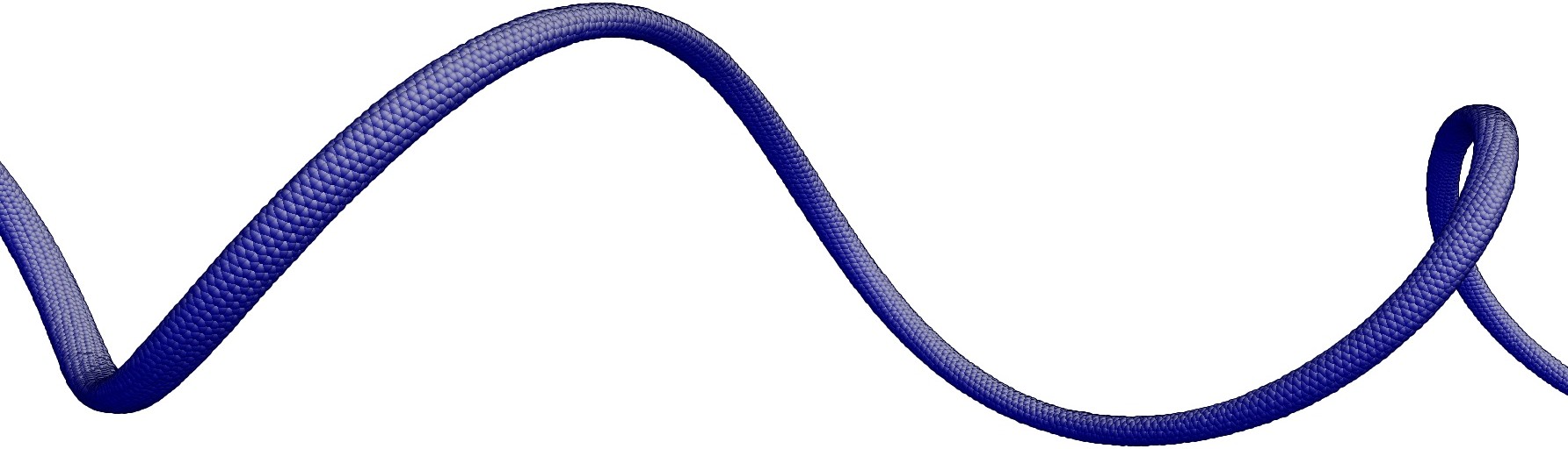
Figure 1: The distorted shape, i.e., the eigenmode, of the nanotube due to the transverse acoustic mode, near the long-wavelength limit of a (7, 6) nanotube.

Before we describe our results, we note that the paper [36] shows, numerically, that bending modes with quadratic dispersion exist in quantum wires with rectangular cross section. The existence of only one continuous wave vector makes the wires similar to nanotubes. However, contrary to nanotubes, because of the rectangular cross section, the bending modes are no longer degenerate in wires. Our systematic symmetry-adapted phonon analysis method is able to deal with the degenerate behavior that occurs in nanotubes and clearly illustrates the quadratic dispersion of the TA phonon modes for a force-free tube.

First, we investigate the effect of axial relaxation on the density of states (DOS) and the form of the dispersion relation for the bending modes. Then we numerically show that the slope and curvature of the TA modes correspond to the axial force and bending rigidity, respectively.

Following the procedures outlined in our previous paper[23], the dispersion curves and DOS for a relaxed (force-free) (7,6) SWNT are plotted in Fig. 2. Adding axial force leads to one significant change of the dispersion curves and DOS. That is, the dispersion of low frequency TA modes changes from quadratic to linear in the long wavelength limit (as $k\rightarrow\theta$), where $\theta=0.307\pi$ is the rotation angle of the $(7,6)$ nanotube screw generator. A consequence of the low frequency dispersion curve near $k=\theta$ is that the DOS is singular near $\omega=0$ for the force-free tube, while conversely, it is almost constant for tubes with non-zero force. This effect is illustrated in Fig. 3, by plotting the long wavelength TA phonon dispersion relation near $k=\theta$ for tubes subjected to four different values of axial stress. Here, we define the axial stress as the axial force divided by the force-free circumference of the tube.

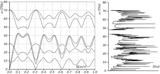
Figure 2: (Left) Dispersion curves and (right) DOS of zero-force axially relaxed (7,6) SWNT as described within the symmetry-adapted objective structures framework of paper[23]

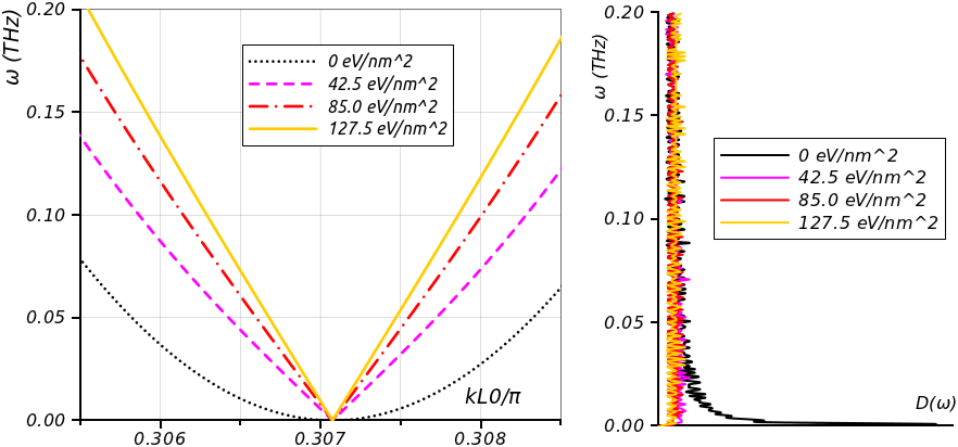
Figure 3: The effect of axial stress on (left) the dispersion relation of the TA phonon modes and (right) the DOS of a (7,6) SWNT

The figure shows clear evidence that the long wavelength TA phonon dispersion behavior is related to the axial stress in the SWNT.

To show more conclusively that the slope and curvature of the long wavelength TA modes have the specific dependence postulated in this paper, we compute (1) the bending modulus of SWNTs as a function of tube diameter, (2) the slope of the long wavelength TA phonon mode dispersion relation as a function of axial stress and tube diameter, and (3) the curvature of the long wavelength TA phonon mode dispersion relations for a force-free SWNT as a function tube diameter.

We compute the energy density versus curvature relation using zero-temperature objective molecular dynamics (based on [22] which allows for the explicit control of curvature through a “bending group parameter”) for armchair nanotubes with different diameters. In particular, we calculate the change in energy density, $\Delta\tilde{\phi}=\Delta\bar{\phi}/(\ell P)$, where $\ell$ is the objective cell length and $P$ is the perimeter of the nanotube. For each radius, we calculate the bending stiffness $\Lambda$ according to

$$\Delta\tilde{\phi}=\frac{1}{2}\Lambda\kappa^{2}\quad\Rightarrow\quad\Lambda=\frac{2\Delta\tilde{\phi}}{\kappa^{2}}.$$ (18)

Figure 4 shows the variation of $\sqrt{\Lambda}$ versus the diameter. It is clear that the bending stiffness scales linearly with the square of the diameter.

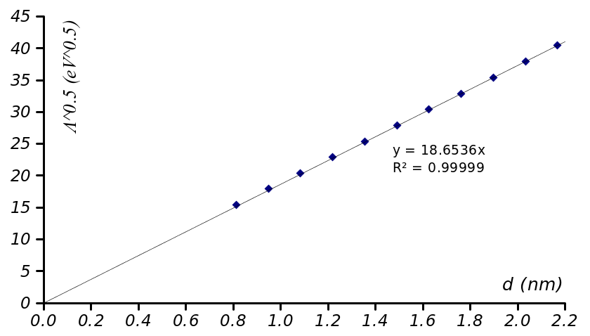
Figure 4: The square root of bending stiffness (calculated by minimizing the energy of armchair nanotubes) versus the diameter of the nanotube. The points are from calculations and the line is a best-fit to the points.

Next, Fig. 5(a) shows the (signed) square of the TA modes’ slope (near $k=\theta$) as a function of axial stress for a variety of tube SWNT types.

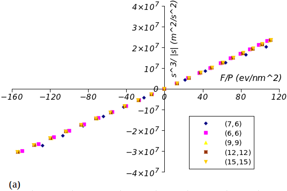
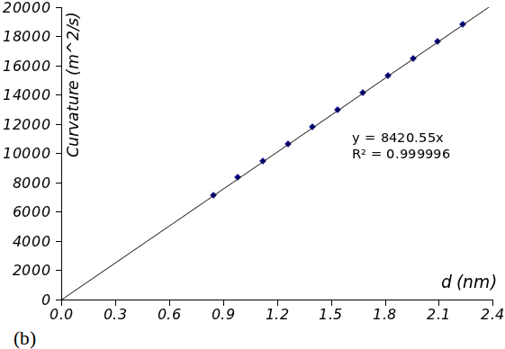
Figure 5: (a) Square of the slope of the TA mode vs. the axial stress. (b) Curvature of the TA mode vs. diameter for various nanotubes ranging from $(6,6)$ to $(16,16)$. The points are from calculations and the line is a best-fit to the points.

This slope was computed from our phonon dispersion calculations using a numerical differentiation algorithm. Finally, in Fig. 5(b) we show the curvature, computed in a similar manner to the slope, for various nanotubes ranging from $(6,6)$ to $(16,16)$ as a function of the tube diameter.

From these figures we can infer the following important results:

• Fig. 5(a) shows that the slope of the TA mode curve does not depend on the specific nanotube. It is linearly related to the square root of the axial force.

• For various nanotubes of different diamters and chiralities, Fig. 5(b) shows that the curvature of the TA mode curve scales linearly with the tube diameter, and Fig. 4 in turn shows that square root of the bending stiffness scales linearly with the tube diameter. Together, these imply that the curvature of the TA mode curve is directly related to the square root of the bending stiffness.

These plots therefore confirm our claim.

5 Simple Continuum Model and Discussion

First we consider the case of a rod that undergoes stretching deformations, but with a pre-stress. This gives us the expected conclusion that the pre-stress plays a role only in determining the equilibrium state around which linearization is conducted. Consider a rod of length $L$ that is extend by an amount $\delta$ and with a pre-stress $\sigma_{0}$. The energy of deformation is, to second order, given by

$$E\sim\sigma_{0}\frac{\delta}{L}+\frac{1}{2}E_{T}\left(\frac{\delta}{L}\right)^{2}+\ldots$$ (19)

Here $E_{T}$ is the extensional modulus at the state of linearization. The natural frequencies from a normal mode analysis will be proportional to the square root of the coefficient of the quadratic term, i.e. $E_{T}^{\frac{1}{2}}$.

Now, to understand the current setting, we examine a beam that undergoes transverse deflections. Consider a beam of length $L$, and impose a bending deformation that causes a relative deflection $\Delta$ between the ends of the beam. A simple accounting of the geometric nonlinearity shows that there is an extensional strain of $\left(1+\left(\frac{\Delta}{L}\right)^{2}\right)^{\frac{1}{2}}-1$ which is simply $\frac{1}{2}\left(\frac{\Delta}{L}\right)^{2}$ to leading order. The energy of deformation is, to second order, given by

$$E\sim\frac{1}{2}\sigma_{0}\left(\frac{\Delta}{L}\right)^{2}+\ldots$$ (20)

The natural frequencies from a normal mode analysis will be proportional to the square root of the coefficient of the quadratic term, i.e. $\sigma_{0}^{\frac{1}{2}}$. When this term is absent, higher-order effects such as bending control the curvature of the TA mode curve.

Therefore, this gives the unusual direct dependence of the normal mode frequencies on the axial force. As the above simple analysis shows, the key to this feature is the geometric nonlinearity of a slender structure.

As our calculations above have shown, the Density of States can also be tuned significantly by applying an axial force. Therefore, it is possible that properties such as heat transfer can be tuned by mechanical means.

References

- [1] J. Yu, R. K. Kalia, and P. Vashishta, “Phonons in graphitic tubules: A tightbinding molecular dynamics study,” Journal of Chemical Physics, vol. 103, p. 6697, 1995.
- [2] R. Saito, T. Takeya, T. Kimura, G. Dresselhaus, and M. S. Dresselhaus, “Raman intensity of single-wall carbon nanotubes,” Physical Review B, vol. 57, p. 4145, 1998.
- [3] M. S. Dresselhaus and P. C. Eklund, “Phonons in carbon nanotubes,” Advances in Physics, vol. 49, pp. 705–814, 2000.
- [4] J. Hone, B. Batlogg, Z. Benes, A. T. Johnson, and J. E. Fischer, “Quantized phonon spectrum of single-wall carbon nanotubes,” Science, vol. 289, pp. 1730–1733, 2000.
- [5] J. Hone, “Phonons and thermal properties of carbon nanotubes,” Topics in Applied Physics, vol. 80, pp. 273–286, 2001.
- [6] J. Maultzsch, S. Reich, C. Thomsen, E. Dobardzic, I. Milosevic, and M. Damnjanovic, “Phonon dispersion of carbon nanotubes,” Solid State Communications, vol. 121, pp. 471–474, 2002.
- [7] D. Sanchez-Portal and E. Hernandez, “Vibrational properties of single-wall nanotubes and monolayers of hexagonal bn,” Physical Review B, vol. 66, p. 235415, 2002.
- [8] J. X. Cao, X. H. Yan, Y. Xiao, Y. Tang, and J. W. Ding, “Exact study of lattice dynamics of single-walled carbon nanotubes,” Physical Review B, vol. 67, p. 045413, 2003.
- [9] E. Dobardzic, I. Milosevic, B. Nikolic, T. Vukovic, and M. Damnjanovic, “Single-wall carbon nanotubes phonon spectra: Symmetry-based calculations,” Physical Review B, vol. 68, p. 045408, 2003.
- [10] D. Sanchez-Portal, E. Artacho, J. M. Soler, A. Rubio, and P. Ordejon, “Ab initio structural, elastic, and vibrational properties of carbon nanotubes,” Physical Review B, vol. 59, p. 12678, 1999.
- [11] V. N. Popov, “Low-temperature specific heat of nanotube systems,” Physical Review B, vol. 66, p. 153408, 2002.
- [12] L.-H. Ye, B.-G. Liu, D.-S. Wang, and R. Han, “Ab initio phonon dispersions of single-wall carbon nanotubes,” Physical Review B, vol. 69, p. 235409, 2004.
- [13] Y. N. Gartstein, “Vibrations of single-wall carbon nanotubes: lattice models and low-frequency dispersion,” Physics Letters A, vol. 327, pp. 83–89, 2004.
- [14] V. N. Popov and P. Lambin, “Radius and chirality dependence of the radial breathing mode and the g-band phonon modes of single-walled carbon nanotubes,” Physical Review B, p. 085407, 2006.
- [15] V. N. Popov and P. Lambin, “Vibrational and related properties of carbon nanotubes,” in Carbon Nanotubes, Springer Netherlands, 2006.
- [16] J. Zimmermann, P. Pavone, and G. Cuniberti, “Vibrational modes and low-temperature thermal properties of graphene and carbon nanotubes: Minimal force-constant model,” Physical Review B, vol. 78, p. 045410, 2008.
- [17] H. Tang, B.-S. Wang, and Z.-B. Su, Graphene Simulation, ch. (10) Symmetry and Lattice Dynamics. Shanghai, China: InTech, 2011.
- [18] V. N. Popov, V. E. V. Doren, and M. Balkanski, “Elastic properties of single-walled carbon nanotubes,” Physical Review B, vol. 15, p. 3078, 2000.
- [19] G. D. Mahan, “Oscillations of a thin hollow cylinder: Carbon nanotubes,” Physical Review B, vol. 65, p. 235402, 2002.
- [20] H. Suzuura and T. Ando, “Phonons and electron-phonon scattering in carbon nanotubes,” Physical Review B, vol. 65, p. 235412, 2002.
- [21] G. D. Mahan and G. S. Jeon, “Flexure modes in carbon nanotubes,” Physical Review B, vol. 70, p. 075405, 2004.
- [22] T. Dumitrica and R. D. James, “Obejective molecular dynamics,” Journal of the Mechanics and Physics of Solids, vol. 55, pp. 2206–2236, Oct. 2007.
- [23] A. Aghaei, K. Dayal, and R. S. Elliott, “Symmetry-adapted phonon analysis of nanostructures,” Journal of the Mechanics and Physics of Solids, 2012. to appear (arXiv preprint arXiv:1209.1593).
- [24] K. Komatsu, “Theory of the specific heat of graphite,” Journal of the Physical Society of Japan, vol. 6, pp. 438–444, 1951.
- [25] K. Komatsu, “Theory of the specific heat of graphite ii,” Journal of the Physical Society of Japan, vol. 10, pp. 346–356, 1955.
- [26] I. M. Lifshitz, “Thermal properties of chain and layered structures at low temperatures,” Zh Eksp Teor Fiz, vol. 22, pp. 475–486, 1952.
- [27] K. Komatsu, “Particle-size effect of the specific heat of graphite at low temperatures,” Journal of Physics and Chemistry of Solids, vol. 6, pp. 380–385, 1958.
- [28] B. T. Kelly and P. L. Walker, “Theory of thermal expandion of a grphite crystal in the semi-continuum model,” Carbon, vol. 8, pp. 211–226, 1970.
- [29] R. A. Suleimanov and N. A. Abdullaev, “The nature of negative linear expansion of graphite crystals,” Carbon, vol. 31, pp. 1011–1013, 1993.
- [30] H. Zabel, “Phonons in layered compounds,” Journal of Physics: Condensed Matter, vol. 13, pp. 7679–7690, 2001.
- [31] G. Savinia, Y. J. Dappec, S. Obergd, J. C. Charliere, M. I. Katsnelsona, and A. Fasolino, “Bending modes, elastic constants and mechanical stability of graphitic systems,” Carbon, vol. 49, pp. 62–69, 2011.
- [32] E. B. Tadmor and R. E. Miller, Modeling Materials: Continuum, Atomistic and Multiscale Techniques. Cambridge University Press, first ed., 2011.
- [33] A. Aghaei and K. Dayal, “Symmetry-adapted non-equilibrium molecular dynamics of chiral carbon nanotubes under tensile loading,” Journal of Applied Physics, vol. 109, no. 12, pp. 123501–123501, 2011.
- [34] A. Aghaei and K. Dayal, “Tension-and-twist of chiral nanotubes: Torsional buckling, mechanical response, and indicators of failure,” Modelling and Simulation in Materials Science and Engineering, 2012.
- [35] J. Tersoff, “Empirical interatomic potential for carbon, with applications to amorphous carbon,” Physical Review Letter, vol. 61, no. 25, pp. 2879–2882, 1988.
- [36] N. Nishiguchi, Y. Ando, and M. N. Wybourne, “Acoustic phonon modes of rectangular quantum wires,” Journal of Physics: Condensed Matter, vol. 9, p. 5751, 1997.