Integrative Model-based clustering of microarray methylation and expression data

Abstract

In many fields, researchers are interested in large and complex biological processes. Two important examples are gene expression and DNA methylation in genetics. One key problem is to identify aberrant patterns of these processes and discover biologically distinct groups. In this article we develop a model-based method for clustering such data. The basis of our method involves the construction of a likelihood for any given partition of the subjects. We introduce cluster specific latent indicators that, along with some standard assumptions, impose a specific mixture distribution on each cluster. Estimation is carried out using the EM algorithm. The methods extend naturally to multiple data types of a similar nature, which leads to an integrated analysis over multiple data platforms, resulting in higher discriminating power.

T1Supported in part by NSF Grant DMS-08-05865.

, , and

1 Introduction

Epigenetics refers to the study of heritable characteristics not explained by changes in the DNA sequence. The most studied epigenetic alteration is cytosine (one of the four bases of DNA) methylation, which involves the addition of a methyl group (a hydrocarbon group occurring in many organic compounds) to the cytosine. Cytosine methylation plays a fundamental role in epigenetically controlling gene expression, and studies have shown that aberrant DNA methylation patterning occurs in inflammatory diseases, aging, and is a hallmark of cancer cells [Rodenhiser and Mann (2006); and Figueroa et al. (2010)]. Figueroa et al. (2010) performed the first large-scale DNA methylation profiling study in humans, where they hypothesized that DNA methylation is not randomly distributed in cancer but rather is organized into highly coordinated and well-defined patterns, which reflect distinct biological subtypes. Similar observations had already been made for expression data [Golub et al. (1999); Armstrong et al. (2002)]. Identifying such biological subtypes through abnormal patterns is a very important task, as some of these malignancies are highly heterogeneous, presenting major challenges for accurate clinical classification, risk stratification and targeted therapy. The discovery of aberrant patterns in subjects can identify tumors or disease subtypes and lead to a better understanding of the underlying biological processes, which in turn can guide the design of more specifically targeted therapies. Due to the biological interaction between methylation and expression, biologists hope to optimize the amount of biological information about cancer malignancies by borrowing strength across both platforms. As an example Figueroa et al. (2008) showed that the integration of gene expression and epigenetic platforms could be used to rescue genes that were biologically relevant but had been missed by the individual analyses of either platform separately.

In this article we propose a model-based approach to clustering such high-dimensional microarray data. In particular, we build finite mixture models that guide the clustering. These types of models have been shown to be a principled statistical approach to practical issues that can come up in clustering [McLachlan and Basford (1988); Banfield and Raftery (1993); Cheeseman and Stutz (1995); Fraley and Raftery (1998, 2002)]. The motivating application is the cluster analysis of Figueroa et al. (2010), which focused on patients with Acute Myeloid Leukemia (AML). Both methylation and expression data are available and we develop a clustering method that can be applied to both data types separately. Furthermore, we extend our methodology to facilitate an integrated cluster analysis of both data platforms simultaneously. Although the methods are designed for these particular applications, we expect that they can be applied to other types of microarray data, such as ChIP-chip data.

A lot of attention has been given to classification based on gene expression profiles and more recently based on methylation profiles. Siegmund, Laird and Laird-Offringa (2004) give an overview and comparison of several clustering methods on DNA methylation data. They point out that among biologists, agglomerative hierarchical cluster analysis is popular. However, they argue in favor of model-based clustering methods over nonparametric approaches and propose a Bernoulli-lognormal model for the discovery of novel disease subgroups. This model had previously been applied by Ibrahim, Chen and Gray (2002) to identify differentially expressed genes and profiles that predict known disease classes. More recently, Houseman et al. (2008) proposed a Recursively Partitioned Mixture Model algorithm (RPMM) for clustering methylation data using beta mixture models [Ji et al. (2005)]. They proposed a beta mixture on the subjects and the objective was to cluster subjects based on posterior class membership probabilities. The RPMM approach is a model-based version of the HOPACH clustering algorithm developed in van der Laan and Pollard (2003).

In high-dimensional data clustering is often performed on a smaller subset of the variables. In fact, as pointed out in Tadesse, Sha and Vannucci (2005), using all variables in high-dimensional clustering analysis has proven to give misleading results. There is some literature on the problem of simultaneous clustering and variable selection [Friedman and Meulman (2003); Tadesse, Sha and Vannucci (2005); Kim, Tadesse and Vannucci (2006)]. However, most statistical methods cluster the data only after a suitable subset has been chosen. An example of such practice is McLachlan, Bean and Peel (2002), where the selection of a subset involves choosing a significance threshold for the covariates. That is also essentially what Houseman et al. (2008) and Figueroa et al. (2010) did, but they selected a subset of the most variable DNA fragments. In this paper we present an integrated model-based hierarchical clustering algorithm that clusters samples based on multiple data types on the most variable features. There is of course a clear advantage of automated variable selection methods such as in Tadesse, Sha and Vannucci (2005). However, the implementation of such methods seems far from straightforward and due to the popularity of hierarchical algorithms among biologists [Kettenring (2006) concluded that hierarchical clustering was by far the most widely used form of clustering in the scientific literature], there is a clear benefit in having a simple hierarchical algorithm that can handle multiple data types.

The article is organized as follows. In Section 2 we describe the features of the motivating data set. In Section 3 we construct the model as a mixture of Gaussian densities, which leads to a specific mixture likelihood that serves as an objective function for clustering. We also introduce individual specific parameters to account for subject to subject variability within clusters (i.e., the array effect). In Section 4 we present two model-based clustering algorithms. The first algorithm is a hierarchical clustering algorithm that can be used to find a good candidate partition. The second clustering algorithm is an iterative algorithm that is designed to improve upon any initial partition. The likelihood model can be applied to classification of new subjects and in Section 5 we describe a discriminant rule for this purpose. In Section 6 we extend the model to account for multiple data platforms and in Sections 7 and 8 we apply the methods to real data sets, which involve both methylation and expression data. We conclude the article with a discussion in Section 9.

2 Motivating data

The Erasmus data were obtained from AML samples collected at Erasmus University Medical Center (Rotterdam) between 1990 and 2008 and involve DNA methylation and expression profiles of $344$ patient specimens. For each specimen it was confirmed that $>$90% of the cells were blasts (leukemic cells). Description of the sample processing can be found in Valk et al. (2004) and data sets are available in GEO, http://www.ncbi.nlm.nih.gov/geo/, with accession numbers GSE18700 for the methylation data and GSE$6891$ for the expression data. The gene expression profiles of the AML samples were determined using oligonucleotide microarrays (Affymetrix U133Plus2.0 GeneChips) and were normalized using the rma normalization method of Irizarry et al. (2003). The processed data involved 54,675 probe sets and demonstrated a right skewed distribution of the expression profiles for each subject; see Supplementary Figure 1 in the supplemental article [Kormaksson et al. (2012)]. The methylation profiles of the AML samples were determined using high density oligonucleotide genomic HELP arrays from NimbleGen Systems that cover 25,626 probe sets at gene promoters, as well as at imprinted genes. Briefly, genomic DNA is isolated and digested by the enzymes HpaII and MspI, separately. While HpaII is only able to cut the DNA at its unmethylated recognition motif (genomic sequence 5^′-CCGG-3^′), MspI cuts the DNA at any HpaII site whether methylated or unmethylated. Following PCR, the HpaII and MspI digestion products are labeled with different fluorophores and then cohybridized on the microarray. This results in two average signal intensities that measure the relative abundances (in a population of cells) of MspI and HpaII at each probe set. The data are preprocessed and normalized using the analytical pipeline of Thompson et al. (2008) and the final quantity of interest is $\log(\mathrm{HpaII}/\mathrm{MspI})$. Note that although theoretically HpaII should always be less than MspI, complex technical aspects that arise during the preparation and hybridization of these samples may result in an enrichment of the HpaII signal over that of MspI. Therefore, the log-ratio does not have a one-to-one correspondence with percent methylation at a given probe set but rather provides a relative methylation value that correlates with actual percentage value (see lower left panel of Figure 1).

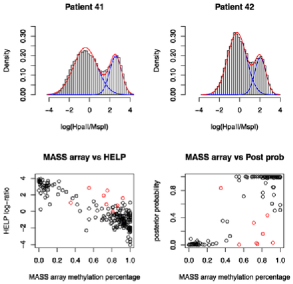
Figure 1: Upper panel: A histogram of the log signal ratio, $\log(\mathrm{HpaII}/\mathrm{MspI})$, for patients number $41$ and $42$ in the Erasmus data set, along with two component Gaussian mixture fits. Lower panel: Left graph shows HELP methylation values plotted against more accurate MASS array methylation percentages. Right graph shows that the posterior probabilities from a two component Gaussian mixture classifies probe sets well into low and high methylation.

In what follows, notation will be based on the HELP methylation data. However, if we abstract away from this particular application, the terminology can be adapted to other microarray data such as gene expression. Let $y_{ij}$ denote the continuous response $\log(\mathrm{HpaII}_{ij}/\mathrm{MspI}_{ij})$ for subject $i=1,\ldots,n$, and probe set $j=1,\ldots,G$. Lower values of $y_{ij}$ indicate that probe set $j$ has high levels of methylation (in a population of cells) for subject $i$, whereas higher values indicate low levels of methylation. In the upper panel of Figure 1 we see bimodal histograms of the methylation profiles for two patients in the AML data set along with two component Gaussian mixture fits. In Supplementary Figure 2 of the supplemental article [Kormaksson et al. (2012)] we see density profiles for all $344$ samples stratified by clusters. There is a large microarray effect in the methylation data, but we observe that all profiles are either skewed or exhibit a bimodal behavior. The lower left panel of Figure 1 shows how the HELP assay correlates with methylation percentages obtained using the more accurate, but much more expensive, quantitative single locus DNA methylation validation MASS Array [see Figueroa et al. (2010)]. It is clear that the HELP values are forming two clusters of relatively low or high methylation levels with some noise in the percentage range $[20\%,80\%]$. This apparent dichotomization inspires modeling each individual profile, $\mathbf{y}_{i}=(y_{i1},\ldots,y_{iG})^{\prime}$, with a two component mixture distribution and normality is assumed for each component due to its flexibility and ease of implementation. We know of no biological mechanism that would imply normality, however, the assumption gives consistent and reasonable fits of the individual methylation profiles (see upper panel of Figure 1).

3 Model specification

By dichotomizing the methylation process we can cluster the probe sets into high or low methylation for each patient $i$ by applying a two component Gaussian mixture model. Let $\mathcal{C}$ denote the true partition of the subject set, $[n]=\{1,\ldots,n\}$. We assume that on any given probe set $j$, all subjects sharing a cluster $c\in\mathcal{C}$ have the same relative methylation status (high or low), and introduce for each cluster $c$ a single latent indicator vector, $\mathbf{w}_{c}=(w_{c1},\ldots,w_{cG})^{\prime}$, with

$$\qquad w_{cj}=\cases{\displaystyle 1,&\quad if $j$ has high methylation for all subjects in cluster $c$,\cr\displaystyle 0,&\quad if $j$ has low methylation for all subjects in cluster $c$.}$$ (1)

It is well known that methylation does exhibit biological variability from individual to individual. However, it is biologically reasonable to expect consistency in relative methylation patterns for patients that share the same disease subtype. Define $\bm{\theta}_{i}=(\mu_{1i},\sigma_{1i}^{2},\mu_{2i},\sigma_{2i}^{2})^{\prime}$ and assume that the observed data, $\mathbf{y}=(\mathbf{y}_{1}^{\prime},\ldots,\mathbf{y}_{n}^{\prime})^{\prime}$, given the unobserved methylation indicators, $\mathbf{w}=(\mathbf{w}_{1}^{\prime},\ldots,\mathbf{w}_{K}^{\prime})^{\prime}$ ($K$ being the number of clusters), arise from the following density:

$$f(\mathbf{y}|\mathbf{w},\bm{\theta})=\prod_{c\in\mathcal{C}}\prod_{i\in c}f(\mathbf{y}_{i}|\mathbf{w}_{c},\bm{\theta}_{i}),$$ (2)

with

$$f(\mathbf{y}_{i}|\mathbf{w}_{c},\bm{\theta}_{i})=\prod_{j=1}^{G}\phi(y_{ij}|\mu_{1i},\sigma_{1i}^{2})^{w_{cj}}\phi(y_{ij}|\mu_{2i},\sigma_{2i}^{2})^{1-w_{cj}},$$ (3)

where $\phi$ denotes the normal density and $\bm{\theta}=(\bm{\theta}_{1}^{\prime},\ldots,\bm{\theta}_{n}^{\prime})^{\prime}$. We refer to the density in (2) as the classification likelihood of the observed data [Scott and Symons (1971); Symons (1981); Banfield and Raftery (1993)] and assume $\mu_{1i}<\mu_{2i}$ for all $i$. We interpret $\bm{\theta}_{i}$ as the individual specific means and variances of the high and low methylation probe sets, respectively. Note that this setup is different from the usual model-based clustering setup where we have cluster specific parameters only. However, due to array effects, it is reasonable and in fact necessary to require different parameters for different subjects. In the upper panel of Figure 1 we see histograms and fits for two patients that both have chromosomal inversions at chromosome $16$, inv($16$) (inversions refer to when genetic material from a chromosome breaks apart and then, during the repair process, it is re-inserted back but the genetic sequence is inverted from its original sense). These two patients cluster together under various clustering algorithms, including the model-based algorithm presented below. However, the two distributions are clearly not equal.

We put a Bernoulli prior on the latent methylation indicators in (1):

$$f(\mathbf{w})=\prod_{c\in\mathcal{C}}\prod_{j=1}^{G}\pi_{1c}^{w_{cj}}\pi_{0c}^{1-w_{cj}},\qquad\pi_{0c}+\pi_{1c}=1,$$ (4)

where $\pi_{1c}$ and $\pi_{0c}$ denote the proportions of probe sets that have high and low methylation, respectively, in cluster $c$. From (2) and (4) it is clear that the complete data density is

$$f(\mathbf{y},\mathbf{w})=\prod_{c\in\mathcal{C}}\prod_{j=1}^{G}\biggl{(}\pi_{1c}\prod_{i\in c}\phi(y_{ij}|\mu_{1i},\sigma_{1i}^{2})\biggr{)}^{w_{cj}}\biggl{(}\pi_{0c}\prod_{i\in c}\phi(y_{ij}|\mu_{2i},\sigma_{2i}^{2})\biggr{)}^{1-w_{cj}},$$ (5)

and if we integrate out the latent variable $\mathbf{w,}$ we arrive at the marginal likelihood

$$L_{\mathcal{C}}(\bm{\Psi})=\prod_{c\in\mathcal{C}}\prod_{j=1}^{G}\biggl{(}\pi_{1c}\prod_{i\in c}\phi(y_{ij}|\mu_{1i},\sigma_{1i}^{2})+\pi_{0c}\prod_{i\in c}\phi(y_{ij}|\mu_{2i},\sigma_{2i}^{2})\biggr{)},$$ (6)

where $\bm{\Psi}=\{(\pi_{1c})_{c\in\mathcal{C}},(\mu_{1i},\sigma_{1i}^{2},\mu_{2i},\sigma_{2i}^{2})_{i}\}$ denotes the set of parameters. This likelihood can be used as an objective function for determining the goodness of different partitions and the maximization of (6) is carried out with the EM algorithm of Dempster, Laird and Rubin (1977). Note that $L_{\mathcal{C}}$ can be written as a product, $\prod_{c\in\mathcal{C}}L_{c}$, where $L_{c}$ denotes the likelihood contribution of cluster $c$. Thus, maximizing $L_{\mathcal{C}}$ can be achieved by maximizing $L_{c}$ independently for all $c\in\mathcal{C}$. Details of the maximization algorithm are provided in Supplementary Appendix B of the supplemental article [Kormaksson et al. (2012)].

Remark 1.

The premise of the clustering algorithm presented in Section 4 is to cluster subjects together that have similar methylation patterns. Similarities across the genome in the posterior probabilities of high/low methylation guide which subjects are clustered together and, thus, if the posterior probability predictions reflect the data well, the clustering algorithm should perform well. In the lower right panel of Figure 1 we see that the posterior probabilities of high methylation fit very well with the actual percentage values.

Remark 2.

When we allow for unequal variances $\sigma_{1i}^{2}\neq\sigma_{2i}^{2}$, the likelihood in (6) is unbounded and does not have a global maximum. This can be seen by setting one of the means equal to one of the data points, say, $\mu_{1i}=y_{ij}$, for some $i,j$. Then the likelihood approaches infinity as $\sigma_{1i}^{2}\rightarrow 0+$. However, McLachlan and Peel (2000), using the results of Kiefer (1978), point out that, even though the likelihood is unbounded, there still exists a consistent and asymptotically efficient local maximizer in the interior of the parameter space. They recommend running the EM algorithm from several different starting values, dismissing any spurious solution (on its way to infinity), and picking the parameter values that lead to the largest likelihood value.

Remark 3.

Note that the likelihood in (6) is identifiable except for the standard and unavoidable label switching problem in finite mixture models [see, e.g., McLachlan and Peel (2000)]. Furthermore, there exists a sequence of consistent local maximizers, as $G\rightarrow\infty$. This becomes more evident if one recognizes that the expression for a single cluster $c$ can be written as a multivariate normal mixture

$$L_{c}=\prod_{j=1}^{G}\bigl{(}\pi_{1c}\phi(\mathbf{y}_{cj}|\bm{\mu}_{1c},\bm{\Sigma}_{1c})+\pi_{0c}\phi(\mathbf{y}_{cj}|\bm{\mu}_{2c},\bm{\Sigma}_{2c})\bigr{)},$$

where $\mathbf{y}_{cj}=(y_{1j},\ldots,y_{n_{c}j})^{\prime}$, $\mu_{kc}=(\mu_{k1},\ldots,\mu_{kn_{c}})^{\prime}$ and $\bm{\Sigma}_{kc}=\operatorname{diag}(\sigma_{ki}^{2})_{i=1}^{n_{c}}$, $k=1,2$ (assuming for convenience that $i=1,\ldots,n_{c}$ are the members of cluster $c$). Standard theory thus applies [see McLachlan and Peel (2000)].

Remark 4.

The correlation structure of high-dimensional microarray data is complicated and hard to model. Thus, we assume independence across variables in the likelihood (6) even though it may not be the absolutely correct model. However, we can view (6) as a composite likelihood [see Lindsay (1988)] which yields consistent parameter estimates but with a potential loss of efficiency. The correlations observed in microarray data are usually mild and involve only a few and relatively small groups of genes that have moderate or high within-group correlations. In Supplementary Appendix A of the supplemental article [Kormaksson et al. (2012)] we perform a simulation study to get a sense of how robust our algorithm is to this independence assumption. The results indicate that with a sparse overall correlation structure in which genes tend to group into many small clusters with moderate to high within-group correlations, our algorithm is not affected by assuming independence across variables. However, there is some indication that with larger groups of genes with very extreme within-group correlations the algorithm will break down. In microarray data such extreme correlation structures are not to be expected on a global scale and, therefore, we believe that the independence assumption is quite reasonable.

4 Model-based clustering

Our clustering criterion involves finding the partition that gives the highest maximized likelihood $L_{\mathcal{C}}$ as given in (6). This provides us with a model selector, as we can compare the maximized likelihoods of any two candidate partitions. In theory we would like to maximize $L_{\mathcal{C}}$ with respect to all possible partitions of $[n]$ and simply pick the one resulting in the highest likelihood. However, as this is impossible for even moderately large $n$, we propose two clustering algorithms. In Section 4.1 we propose a simple hierarchical clustering algorithm, and in Section 4.2 we propose an iterative algorithm that is designed to improve upon any initial partition.

4.1 Hierarchical clustering algorithm

In this subsection we describe a simple hierarchical algorithm that attempts to find the partition that maximizes $L_{\mathcal{C}}$ as given in (6). Heard, Holmes and Stephens (2006) used a similar approach, but they constructed a hierarchical Bayesian clustering algorithm that seeks the clustering leading to the maximum marginal posterior probability. The algorithm can be summarized in the following steps: [3.]

We start with the partition where each subject represents its own cluster, $\mathcal{C}_{1}=\{\{1\},\ldots,\{n\}\}$, and calculate the maximized likelihood, $L_{\mathcal{C}_{1}}$. Note that this likelihood can be written as a product $L_{\mathcal{C}_{1}}=\prod_{i}L_{\{i\}}$ and, thus, the first step involves maximizing $L_{\{i\}}$ for each $i=1,\ldots,n$. This is achieved by fitting a two-component Gaussian mixture to each of the $n$ individual profiles. As mentioned in Remark 2, each fit can be obtained by using the EM algorithm starting from several different initial values and finding a local maximum. It is important that the user verifies these initial individual fits before proceeding with the hierarchical algorithm. For example, by going through the $344$ methylation profile fits of the Erasmus data, one by one, we observe pleasing fits. The upper panel of Figure 1 gives examples of two such profile fits.

Next we merge the two subjects that leads to the highest value of $L_{\mathcal{C}}$ and denote the maximized likelihood value by $L_{\mathcal{C}_{2}}$. Note that there are ${n\choose 2}$ many ways of merging two subjects at this step. However, since we already obtained fits for $L_{\{i\}}$, $i=1,\ldots,n$, at Step 1, we only need to maximize $L_{\{i,i^{\prime}\}}$, for all pairs $(i,i^{\prime})$ and find the pair that maximizes

$$\ell_{\mathcal{C}_{2}}=\ell_{\mathcal{C}_{1}}-\bigl{(}\ell_{\{i\}}+\ell_{\{i^{\prime}\}}\bigr{)}+\ell_{\{i,i^{\prime}\}},$$

where $\ell$ denotes the loglikelihood. Even though we are applying several EM algorithms, the complexity of each algorithm is low since it only involves two subjects at a time.

We continue merging clusters under this maximum likelihood criteria, at each step making note of the maximized likelihood, until we are left with one cluster containing all $n$ subjects, $\mathcal{C}_{n}=[n]$. Among the $n$ partitions that are obtained, we pick the partition that has the highest value of $L_{\mathcal{C}}$. Note that the likelihood value may either increase or decrease at each step. This provides us with a method that automatically determines the number of clusters. It is our experience that the individual parameter estimates $(\mu_{1i},\sigma_{1i}^{2},\mu_{2i},\sigma_{2i}^{2})_{i}$ do not change much at each merging step of the hierarchical algorithm. Thus, if the initial estimates provide good fits for all the individual profiles, the algorithm can be expected to perform well. Furthermore, by using the individual parameter estimates at a previous merging step as initial values at the next step, each EM algorithm converges very quickly, which is essential since the total number of EM algorithms that are conducted is of the order $O(n^{2})$. For the data sets that we consider in this article, the hierarchical algorithm takes anywhere from a couple of minutes to run, for the smallest data set in Section 8.1 ($n=14$), up to a couple of hours for the Erasmus high-dimensional data set of Section 7.1 ($n=344$), using a regular laptop. However, it should be noted that our R code is neither optimized nor precompiled to a lower level programming language at this stage.

4.2 Iterative clustering algorithm

The hierarchical algorithm results in a partition that serves as a good initial candidate for the true partition. In this subsection we present an iterative algorithm that is designed to improve upon any initial partition. We introduce cluster membership indicators for the subjects in order to develop an EM algorithm for clustering subjects under the assumption of a fixed number of clusters. Define for each subject $i=1,\ldots,n$ and cluster $c\in\mathcal{C}$

$$X_{ic}=\cases{\displaystyle 1,&\quad if subject $i$ is in cluster $c$,\cr\displaystyle 0,&\quad otherwise,}$$

and let $\mathbf{X}_{i}=(X_{ic})_{c\in\mathcal{C}}$. Assume $\mathbf{X}_{1},\ldots,\mathbf{X}_{n}$ are i.i.d. Multinom$\{1,\mathbf{p}=(p_{c})_{c\in\mathcal{C}}\}$, so the density of $\mathbf{X}=(\mathbf{X}_{1}^{\prime},\ldots,\mathbf{X}_{n}^{\prime})^{\prime}$ is

$$f(\mathbf{X})=\prod_{i=1}^{n}\prod_{c\in\mathcal{C}}p_{c}^{X_{ic}},\qquad\sum_{c\in\mathcal{C}}p_{c}=1.$$ (7)

These cluster membership indicators fully define the partition $\mathcal{C}$ and we note that the classification likelihood in (2) can be written as

$$f(\mathbf{y}|\mathbf{X})=\prod_{c\in\mathcal{C}}\prod_{i=1}^{n}f(\mathbf{y}_{i}|\mathbf{w}_{c},\bm{\theta}_{i})^{X_{ic}}.$$ (8)

Multiplying (7) and (8) together and integrating out $\mathbf{X}$, we arrive at the marginal likelihood

$$f(\mathbf{y};\bm{\Psi})=\prod_{i=1}^{n}\sum_{c\in\mathcal{C}}p_{c}f(\mathbf{y}_{i}|\mathbf{w}_{c},\bm{\theta}_{i}),$$ (9)

where $\bm{\Psi}=\{(p_{c})_{c\in\mathcal{C}},(\mathbf{w}_{c})_{c\in\mathcal{C}},\bm{\theta}_{i}=(\mu_{1i},\sigma_{1i}^{2},\mu_{2i},\sigma_{2i}^{2})_{i}\}$ involves both the continuous parameters and the discrete indicators, $\mathbf{w}$, which we now assume are fixed. We make this assumption because if $\mathbf{w}$ is random as in (4), the joint posterior distribution of $(\mathbf{w},\mathbf{X})$ is highly intractable and an EM algorithm based on (8) would be problematic.

The likelihood in (9) is that of a finite mixture model and can be maximized using the EM algorithm. We detail the maximization procedure in Supplementary Appendix B of the supplemental article [Kormaksson et al. (2012)]. In short, let $\mathbf{X}^{(0)}$ denote the clustering labels corresponding to a candidate partition. Using $\mathbf{X}^{(0)}$ as an initial partition, we run an EM algorithm that converges to a local maximum of (9). Once the mixture model has been fitted, a probabilistic clustering of the subjects can be obtained through the fitted posterior expectations of cluster membership for the subjects, $(E[X_{ic}|\mathbf{y}])_{i,c}$ [see McLachlan and Peel (2000)]. Essentially, a subject will be assigned to the cluster to which it has the highest estimated posterior probability of belonging. We have found empirically that the derived partition not only results in a higher value of (9) but also in the objective likelihood (6), but we do not have a theoretical justification for this. A good clustering strategy is to come up with a few candidate partitions, with varying numbers of clusters, and run the EM algorithm using these partitions as initial partitions. Each resulting partition will be a local maximum of (9), but we choose the partition with the highest value of the original objective function (6). Good initial partitions can be found by running the hierarchical algorithm of Section 4.1 or applying one of the more standard clustering algorithms.

5 Classification

The construction of a likelihood for any given partition of the subjects also provides a powerful tool for classification. Assume we have methylation data on $n$ subjects and we know which class each subject belongs to, that is, we know the true $\mathcal{C}$. A by-product of maximizing the likelihood in (6) with the EM algorithm [detailed in Supplementary Appendix B of the supplemental article, Kormaksson et al. (2012)] is posterior predictions of the latent indicators, $(\mathbf{\hat{w}}_{c})_{c\in\mathcal{C}}$, which we round to either $0$ or $1$. Given these estimated methylation indicators, the conditional likelihood of a new observation $(y_{ij})_{j}$, on the assumption that $i\in c$, is given by

$$L_{c}(\bm{\theta}_{i})=\prod_{j=1}^{G}\phi(y_{ij}|\mu_{1i},\sigma_{1i}^{2})^{\hat{w}_{cj}}\phi(y_{ij}|\mu_{2i},\sigma_{2i}^{2})^{1-\hat{w}_{cj}}.$$ (10)

The discriminant likelihood, $L_{c}$, is maximized with respect to the individual specific parameters at

$$\hat{\mu}_{1i} = \frac{\sum_{j}\hat{w}_{cj}y_{ij}}{\sum_{j}\hat{w}_{cj}},\qquad\hat{\sigma}^{2}_{1i}=\frac{\sum_{j}\hat{w}_{cj}(y_{ij}-\hat{\mu}_{1i})^{2}}{\sum_{j}\hat{w}_{cj}},$$

$$\hat{\mu}_{2i} = \frac{\sum_{j}(1-\hat{w}_{cj})y_{ij}}{\sum_{j}(1-\hat{w}_{cj})},\qquad\hat{\sigma}^{2}_{2i}=\frac{\sum_{j}(1-\hat{w}_{cj})(y_{ij}-\hat{\mu}_{2i})^{2}}{\sum_{j}(1-\hat{w}_{cj})}.$$

By substituting these estimates into (10) we arrive at the following discriminant rule:

$$i\in c\qquad\mbox{if }L_{c}(\hat{\bm{\theta}}_{i}(\mathbf{\hat{w}}_{c}))>L_{c^{\prime}}(\hat{\bm{\theta}}_{i}(\mathbf{\hat{w}}_{c^{\prime}}))\mbox{ for all }c^{\prime}\neq c.$$ (11)

6 Extension to multiple platforms

In this section we discuss how to extend the methods of this paper to account for multiple data types as long as each data type can reasonably be modeled by the model described in Section 3. For subject $i=1,\ldots,n$ let $y_{ijk}$ denote the signal response of the $j$th variable, $j=1,\ldots,G_{k}$, on platform $k=1,\ldots,m$. As before, we let $\mathcal{C}$ denote the true partition of the $n$ subjects. We assume subjects in a given cluster $c\in\mathcal{C}$ have identical activity (methylation, expression, etc.) profiles on each platform $k=1,\ldots,m$ independently and define a cluster and platform specific indicator for each variable

$$w_{cjk}=\cases{\displaystyle 1,&\quad if variable $j$ on platform $k$ is active in cluster $c$,\cr\displaystyle 0,&\quad if variable $j$ on platform $k$ is inactive in cluster $c$.}$$

Define $\mathbf{w}_{c}=(w_{cjk})_{j,k}$ and let $\mathbf{y}_{i}=(y_{ijk})_{j,k}$ denote the vector of observed activity profiles of subject $i$ across platforms. Let $\bm{\theta}_{i}=(\mu_{1ik},\sigma_{1ik}^{2},\mu_{2ik},\sigma_{2ik}^{2})_{k=1}^{m}$ denote the subject specific mixture parameters. We assume that the observed data, $\mathbf{y}=(\mathbf{y}_{1}^{T},\ldots,\mathbf{y}_{n}^{T})^{T}$, given the unobserved activity indicators, $\mathbf{w}=(\mathbf{w}_{c})_{c\in\mathcal{C}}$, arise from the following density:

$$f(\mathbf{y}|\mathbf{w},\bm{\theta})=\prod_{c\in\mathcal{C}}\prod_{i\in c}f(\mathbf{y}_{i}|\mathbf{w}_{c},\bm{\theta}_{i}),$$

where the conditional density of $\mathbf{y}_{i}$, on the assumption that $i\in c$, is given by

$$f(\mathbf{y}_{i}|\mathbf{w}_{c},\bm{\theta}_{i})=\prod_{k=1}^{m}\prod_{j=1}^{G_{k}}\phi(y_{ijk}|\mu_{1ik},\sigma_{1ik}^{2})^{w_{cjk}}\phi(y_{ijk}|\mu_{2ik},\sigma_{2ik}^{2})^{1-w_{cjk}}.$$

We can either assume that the activity indicators for cluster $c$ are fixed as in subection 4.2, or independent Bernoullis, both across platforms and variables,

$$f(\mathbf{w}_{c})=\prod_{k=1}^{m}\prod_{j=1}^{G_{k}}\pi_{1ck}^{w_{cjk}}\pi_{0ck}^{1-w_{cjk}},\qquad\pi_{1ck}+\pi_{0ck}=1,$$

where $\pi_{1ck}$ represents the proportions of variables on platform $k$ that are active in cluster $c$. The likelihood in this integrated framework is identical to the one given in (6), except we now have an additional product across platforms $k$. The methods presented in Sections 4 and 5 thus extend to multiple platforms in a straightforward manner.

7 Identifying subtypes of AML

Figueroa et al. (2010) performed the first large-scale DNA methylation profiling study in humans using the Erasmus data described in Section 2. They clustered patients using hierarchical correlation based clustering on a subset of the most variable probe sets. Using unsupervised clustering, they were able to classify the patients into known and well-characterized subtypes as well as discover novel clusters. In Section 7.1 we report our clustering results on the data and compare to those of Figueroa et al. (2010). We ran a cluster analysis on both methylation and expression data separately as well as an integrative cluster analysis on both platforms simultaneously. In Section 7.2 we present results from a discriminant analysis study in which we classified an independent validation data set using the methods of Section 5.

7.1 Clustering results

Figueroa et al. (2010) hierarchically clustered the $n=344$ patients (methylation profiles only) on a subset of the 3745 most variable probe sets, using 1-correlation distance and Ward’s agglomeration method. These were probe sets that exceeded a standard deviation threshold of $1$. We ran the hierarchical algorithm of Section 4.1 on the same subset to obtain an initial partition. Among the $344$ candidate partitions, obtained at each merging step, the loglikelihood was maximized at $K=17$ clusters, but to avoid singletons we chose a partition with $K=16$, the same number of clusters Figueroa et al. (2010) chose. We then applied the iterative algorithm of Section 4.2 in an attempt to improve upon the initial partition. We denote the resulting partition “M” (Methylation). We repeated this process separately for the expression data using the 3370 most variable probe sets, or those that exceeded a standard deviation threshold of $0.5$. This resulted in a partition “E” (Expression) with $K=17$ clusters. Finally, we repeated this process jointly on the 3745 and 3370 probe sets from the methylation and expression data, respectively, resulting in the partition “ME” with $K=14$ clusters.

Figueroa et al. (2010) identified $3$ robust and well-characterized biological clusters and $8$ clusters that were associated with specific genetic or epigenetic lesions. Five clusters seemed to share no known biological features. The three robust clusters corresponded to cases with inversions on chromosome $16$, inv$(16)$, and translocations between chromosomes $15$ and $17$, $t(15;17)$, and chromosomes $8$ and $21$, $t(8;21)$ (translocations refer to when genetic material from two different chromosomes breaks apart and when being repaired, the material from one chromosome is incorrectly attached to the other chromosome instead and vice versa). The World Health Organization has identified these subtypes of AML as indicative of favorable clinical prognosis [see, e.g., Figueroa et al. (2010)]. The remaining $8$ clusters included patients with CEBPA double mutations (two different abnormal changes in the genetic code of the CEBPA gene), CEBPA mutations irrespective of type of mutation, silenced CEBPA (abnormal loss of expression of CEBPA which is not due to mutations in the genetic code), one cluster enriched for 11q23 abnormalities (any type of change in the genetic code that affects position $23$ of the long arm of chromosome $11$) and FAB M5 morphology (specific shape and general aspect of the leukemic cell as defined by the French American British classification system for Acute Leukemias), and four clusters with NPM1 mutations (mutations in the genetic code of the NPM1 gene). A detailed sensitivity and specificity analysis of $6$ of the above $11$ clusters [sample sizes in brackets], inv$(16)$ [$n_{1}=28$], $t(15;17)$ [$n_{2}=10$], $t(8;21)$ [$n_{3}=24$], CEBPA double mutations [$n_{4}=24$], CEBPA silenced AMLs [$n_{5}=8$], and $11q23+\mbox{FAB M5}$ [$n_{6}=7$], is given in Table 1 for the different clustering results. We include the correlation based clustering result (COR) on the methylation data to compare with “M.” The remaining five of the $11$ biological clusters (CEBPA mutations irrespective of type of mutation and the four NPM1 mutation clusters) had sensitivity or specificity below $0.5$ for all four clustering results and were thus excluded from the table. We can see that the model-based approach, “M,” is doing better than the correlation based method, “COR,” for the most part. Aside for sensitivity of $t(8;21)$ ($1$ less false negative) and specificity of inv$(16)$ ($1$ less false positive), the model-based approach has as good or better sensitivity and specificity. The most striking differences are in the numbers of false negatives of CEBPA dm and false positives of $t(8;21)$ where “M” is doing better. Note also that aside for the sensitivity of $11q23+\mbox{FAB M5}$ and specificity of $t(8;21)$, the integrated analysis “ME” always does better than the analyses “M” and “E” separately, with perfect sensitivity and specificity for many of the clusters. Most notably, the integrative analysis is able to perfectly classify the CEBPA double mutants even though both “M” and “E” have quite a few false positives and false negatives. This demonstrates the increased power to identify clusters by sharing information across multiple platforms. As a side product from our clustering algorithm, we obtain posterior probabilities of high methylation/expression, $E[w_{cj}|\mathbf{y}]$, which can be used to order genes in heatmaps to discover subtype specific methylation/expression patterns. In Figure 2 we see heatmaps of the two data sets used for the integrative clustering, “ME,” after rows have been ordered by increasing posterior probabilities (one cluster at a time). Such heatmaps are useful for graphically displaying the distinct methylation/expression patterns that characterize the different subtypes of cancer.

Table 1: The sensitivity and specificity of the clustering results

Subtype	COR	M	E	ME
Sensitivity (# of false negatives in parentheses)
inv($16$) [$n_{1}=28$]	$0.929\ (2)$	$0.964\ (1)$	$0.857\ (4)$	$0.964\ (1)$
$t(15;17)$ [$n_{2}=10$]	$0.800\ (2)$	$0.800\ (2)$	$1.000\ (0)$	$1.000\ (0)$
$t(8;21)$ [$n_{3}=24$]	$0.917\ (2)$	$0.875\ (3)$	$0.917\ (2)$	$0.958\ (1)$
CEBPA dm [$n_{4}=24$]	$0.792\ (5)$	$0.917\ (2)$	$0.75\ (6)$0	$1.000\ (0)$
CEBPA Sil [$n_{5}=8$]	$0.625\ (3)$	$0.875\ (1)$	$1.000\ (0)$	$1.000\ (0)$
$11q23+\mbox{FAB M5}$ [$n_{6}=7$]	$0.857\ (1)$	$0.857\ (1)$	$0.714\ (2)$	$0.714\ (2)$
Specificity (# of false positives in parentheses)
inv($16$) [$n-n_{1}=316$]	$1.000\ (0)$	$0.997\ (1)$	$0.997\ (1)$	$1.000\ (0)$
$t(15;17)$ [$n-n_{2}=334$]	$1.000\ (0)$	$1.000\ (0)$	$1.000\ (0)$	$1.000\ (0)$
$t(8;21)$ [$n-n_{3}=320$]	$0.972\ (9)$	$0.994\ (2)$	$1.000\ (0)$	$0.991\ (3)$
CEBPA dm [$n-n_{4}=320$]	$0.988\ (4)$	$0.988\ (4)$	$0.991\ (3)$	$1.000\ (0)$
CEBPA Sil [$n-n_{5}=336$]	$1.000\ (1)$	$0.997\ (1)$	$0.985\ (5)$	$0.997\ (1)$
$11q23+\mbox{FAB M5}$ [$n-n_{6}=337$]	$0.991\ (3)$	$0.991\ (3)$	$0.991\ (3)$	$0.994\ (2)$

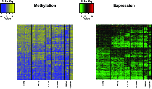
Figure 2: Heatmaps of the methylation and gene expression values for the 6 well-characterized clusters obtained from the integrative clustering (“ME”). Columns correspond to patient samples and rows correspond to genes. On the left heatmap “yellow,” “gray” and “blue” represent low, intermediate and high methylation, respectively. On the right heatmap “green,” “black” and “red” represent low, intermediate and high expression, respectively. Rows are ordered by increasing posterior probabilities of high methylation/expression, $E[w_{cj}|\mathbf{y}]$, first for inv$(16)$, then for $t(8;21)$, $t(15;17)$, CEBPdm, CEBPsil, and finally for 11q23+M5. Rows with equal probabilities for all $6$ clusters (either equal to $1$ or $0$) are excluded to emphasize differences.

7.2 Classification results

A second cohort of patients with AML was available with which we could test the performance of the classification method of Section 5. This second cohort of $n=383$ cases consisted of samples, obtained from patients enrolled in a clinical trial from the Eastern Cooperative Oncology Group (ECOG) (Data are available at http://www.ncbi. nlm.nih.gov/geo/, accession number pending). These patients were similar in characteristics to the Erasmus cohort, with only one exception, all patients were younger than $60$ years of age. Samples were processed in the same way as the Erasmus cohort, and their methylation was used to blindly predict their molecular diagnosis. Using the 3745 most variable probe sets and the clustering result “M” of the previous section, we fit the model (6) on the Erasmus cohort with the EM algorithm. By using the posterior predictions of the methylation indicators, we applied the discriminant rule (11) on each patient in the ECOG data set. Since CEBPA and NPM1 mutation status have not yet been made available for this cohort, only the performance for the prediction of the inv$(16)$, $t(8;21)$, CEBPA silenced, $t(15;17)$ and $11q23+\mbox{FAB M5}$ clusters could be tested. Inv$(16)$ cases were predicted with $100\%$ sensitivity and specificity. The predicted $t(8;21)$ cluster contained $100\%$ of cases positive for this abnormality, and only one $t(8;21)$ case was misclassified to another cluster. Two cases, which had previously been unrecognized as CEBPA silenced AMLs, were predicted by the classification method. One of them was later confirmed to indeed correspond to this molecular subtype by an alternative methylation measurement method. Similarly, one case was believed to have been misclassified as $t(15;17)$ since there were no molecular data confirming the presence of the PML-RARA gene fusion (the abnormal combination of the PML and RARA genes) resulting from this translocation. However, it was later confirmed that both the morphology and the immune diagnosis corresponded to that of an acute promyelocytic leukemia with $t(15;17)$. Finally, the $11q23+\mbox{FAB M5}$ cluster included $9$ of the $14$ patients in the cohort that met these two criteria. There were also $5$ false positives, $3$ of them were M5 cases but did not have $11q23$ abnormalities, $1$ of them harbored the $11q23$ abnormality but corresponded to an M1, and the remaining case corresponded to an M4 case with a hyperdiploid karyotype. A summary of these results is provided in Table 2.

=230pt Subtype Sensitivity Specificity inv($16$) [$n=32$] $1.000\ (0)$ $1.000\ (0)$ $t(15;17)$ [$n=1$] $1.000\ (0)$ $1.000\ (0)$ $t(8;21)$ [$n=28$] $0.964\ (1)$ $1.000\ (0)$ CEBPA Sil [$n=1$] $1.000\ (0)$ $0.997\ (1)$ $11q23+\mbox{FAB M5}$ [$n=14$] $0.643\ (5)$ $0.986\ (5)$

Table 2: The sensitivity and specificity of the classification result. False negatives and false positives are in parentheses

8 Other applications

The clustering method presented in this paper is not restricted to the microarray platforms that the AML samples were processed on. In this section we demonstrate the versatility of our method by applying it to other microarray platforms and show that our algorithm does well in clustering subjects. We also provide a comparison with other existing methods for clustering microarray data.

8.1 Expression in endometrial cancer

In this subsection we analyze the microarray expression data set in Tadesse, Sha and Vannucci (2005). Endometrioid endometrial adenocarcinoma is a gynecologic malignancy typically occurring in postmenopausal women. Identifying distinct subtypes based on common patterns of gene expression is an important problem, as different clinicopathologic groups may respond differently to therapy. Such subclassification may lead to discoveries of important biomarkers that could become targets for therapeutic intervention and improved diagnosis. High density microarrays (Affymetrix Hu6800 chips) were used to study expression of $4$ normal and $10$ endometrioid adenocarcinomas on 7070 probe sets. Probe sets with at least one unreliable reading (limits of reliable detection were set to 20 and 16,000) were removed from the analysis, which resulted in $G=762$ variables. Finally, the data were log-transformed, however, unlike Tadesse, Sha and Vannucci (2005), we chose not to rescale the variables by their range. More details about the data set can be found in Tadesse, Ibrahim and Mutter (2003) and is publicly available at http://endometrium.org.

We hierarchically clustered the samples using the $300$ most variable probe sets and plotted the results in Figure 3. We successfully separated the four normal tissues from the endometrial cancer tissues and the log-likelihood plot suggests that $K=2$. The dendrogram consistently separated the normals and the cancer into two branches for different variance thresholds. However, if we lowered the threshold too much, the loglikelihood was maximized at $K=1$. This makes sense, as including many low variability probe sets might mask the true clustering structure. For comparison, Tadesse, Sha and Vannucci (2005) concluded that $K=3$ and commented that there could possibly be $2$ subtypes of endometrial cancer. However, to the best of our knowledge, this subclustering has not been verified. They also reported clustering results using the COSA algorithm of Friedman and Meulman (2003), which, like our analysis, seemed more suggestive of $K=2$.

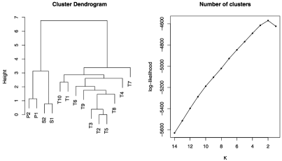
Figure 3: Left panel: Cluster dendrogram for the $2$ normal proliferative (“P”) endometria, $2$ normal secretory (“S”) endometria, and $10$ endometrioid adenocarcinomas (“T”). Right panel: Plot of the number of clusters against log-likelihood.

8.2 Methylation in normal tissues

Houseman et al. (2008) used the RPMM algorithm to cluster a methylation data set consisting of $217$ normal tissues and compared the performance to that of the HOPACH algorithm of van der Laan and Pollard (2003). The RPMM analysis was discussed in more detail in Christensen et al. (2009) and the data made publicly available at the GEO depository with accession number GSE19434 (http://www.ncbi.nlm.nih.gov/geo/). Briefly, DNA was extracted from the tissues, modified with sodium bisulfite, and processed on the Illumina GoldenGate methylation platform. Average fluorescence for methylated ($M$) and unmethylated ($U$) alleles were derived from raw data at $1505$ loci. However, in this study $1413$ loci passed the quality assurance procedures. A total of $11$ tissue types were available, bladder ($n=5$), adult blood ($n=30$), infant blood ($n=55$), brain ($n=12$), cervix ($n=3$), head and neck ($n=11$), kidney ($n=6$), lung ($n=53$), placenta ($n=19$), pleura ($n=18$) and small intestine ($n=5$). Houseman et al. (2008) constructed an average “beta” value from raw data, which they claimed was very close to the quantity $M/(M+U)\in(0,1)$, rendering a beta distributional assumption (assuming $M$ and $U$ follow a gamma distribution) with class and locus specific parameters. We, however, chose to work with the quantity $\log(M/U)$, which fits better with our two component mixture distributional assumption. In order to get a direct comparison with RPMM and HOPACH, we used all $1413$ loci. In Supplementary Figure 3 of the supplemental article [Kormaksson et al. (2012)] we see a plot of cluster number versus loglikelihood, which is maximized at $K=6$ clusters. However, given the relatively small difference between the loglikelihood values at $K=6$, $K=7$, and $K=8$, one could argue that all three clustering results are worthy of consideration. The clusters are cross-classified with tissue type in Table 3.

Table 3: Cross-classification of our clustering result ($K=8$) and tissue type. By merging the top two clusters, and clusters $3$ and $4,$ we obtain the clustering corresponding to $K=6$

Class	Blad	Bl	Br	Cerv	Inf bl	HN	Kid	Lung	Plac	Pleu	Sm int
1	5			2		1		53		18	4
2				1
3							6
4						10					1
5		30
6			12
7					55
8									19

If we compare these results with those obtained with the RPMM algorithm, our result favors few and concise clusters, whereas RPMM is indicative of a total of $23$ subclasses of tissues. The HOPACH clustering algorithm was suggestive of $K=9$ clusters, with $3$ of those clusters representing placenta singletons separated from the main placenta cluster. We present a cross-classification table for both RPMM and HOPACH in Supplementary Table 3 of the supplemental article [Kormaksson et al. (2012)] for comparison [borrowed from Houseman et al. (2008)]. Our method perfectly classifies blood, brain, infant blood, kidney and placenta. For comparison, after bundling subclusters together, RPMM classifies blood and infant blood perfectly, and HOPACH classifies infant blood and placenta perfectly. All three methods have problems distinguishing between bladder, cervical, lung, pleural and small intestine tissues. Overall, our approach seems to outperform HOPACH, and although Houseman et al. (2008) have demonstrated that a few of their tissue-specific subclusters (obtained by RPMM) have verifiable meanings, such as through age difference, it seems that without a further justification of such finer substructure in the data our clustering result is more desirable. As a side note, under the assumption of Houseman et al. (2008) that $M$ and $U$ follow a gamma distribution, it is clear that $\log(M/U)$ will not be a mixture of two Gaussian distributions. The favorable clustering result for this data set suggests that the normality assumption on each mixture component provides a robust and flexible modeling distribution.

9 Discussion

We have proposed a model-based method for clustering microarray data. The methods have been demonstrated to work well on expression data and methylation data separately. An integrated cluster analysis has further shown the power of combining platforms in a joint analysis. We believe this method can be applied to a variety of microarray data types. However, further research is needed to validate the method on different types of data such as ChIP–chip data.

A minor drawback of our method is that it does not allow for automated selection of variables, but rather relies on pre-filtering the data. However, most biologists are still relying on simple clustering algorithms such as $K$-means or standard agglomerative algorithms, due to their simplicity in implementation and interpretation. Thus, having a relatively simple and easily implemented hierarchical algorithm that can integrate multiple platforms and further utilizes the bimodal or skewed structure of the individual profiles, in a model-based manner, has its advantages. For example, the hierarchical algorithm automatically determines the numbers of clusters and provides an easily interpretable dendrogram. Also, as a side product, we obtain posterior probabilities of high methylation/expression, $E[w_{cj}|\mathbf{y}]$, for each cluster $c$ and probe set $j$. By ordering the probe sets with respect to these posterior probabilities and excluding probe sets that are identical across all clusters, we can explore patterns in heatmaps such as in Figure 2.

One of the novelties of our clustering algorithm is the inclusion of individual specific parameters, $(\mu_{1i},\sigma_{1i}^{2},\mu_{2i},\sigma_{2i}^{2})_{i}$, into the model of Section 3, which facilitates the use of our algorithm even in the presence of extreme microarray effects. Since the amount of data we have to estimate these parameters ($G$ observations per subject) highly exceeds the number of subjects ($n$), the estimation of these parameters has not been a problem. However, it is common practice to treat such individual specific parameters as random effects. We have established that with conjugate normal and inverse gamma priors on the above parameters we arrive at a marginal likelihood intractable for maximization. However, we have verified that through such prior specifications we could easily calculate full conditionals in a Bayesian analysis. A Bayesian approach would also prevent us from having to assume the methylation indicators, $\mathbf{w}$, are fixed as in the iterative algorithm of Section 4.2. The reason for that assumption was that the joint posterior distribution of $(\mathbf{w},\mathbf{X})$ is highly intractable. However, full conditionals for each variable separately are easily obtained and are that of Bernoulli and Multinomial, respectively. Running a fully Bayesian analysis might also facilitate an extended algorithm that could include all variables. One might assume that some variables are informative and follow the mixture in (6) with prior probability $p$, whereas other variables are noninformative with prior probability $(1-p)$ and follow the mixture in (6) with $\mathcal{C}=[n]$. There are some challenges that arise in implementing such a fully Bayesian model and those require further research.

References

- Armstrong et al. (2002) {barticle}[pbm] \bauthor\bsnmArmstrong, \bfnmScott A.\binitsS. A., \bauthor\bsnmStaunton, \bfnmJane E.\binitsJ. E., \bauthor\bsnmSilverman, \bfnmLewis B.\binitsL. B., \bauthor\bsnmPieters, \bfnmRob\binitsR., \bauthor\bparticleden \bsnmBoer, \bfnmMonique L.\binitsM. L., \bauthor\bsnmMinden, \bfnmMark D.\binitsM. D., \bauthor\bsnmSallan, \bfnmStephen E.\binitsS. E., \bauthor\bsnmLander, \bfnmEric S.\binitsE. S., \bauthor\bsnmGolub, \bfnmTodd R.\binitsT. R. and \bauthor\bsnmKorsmeyer, \bfnmStanley J.\binitsS. J. (\byear2002). \btitleMLL translocations specify a distinct gene expression profile that distinguishes a unique leukemia. \bjournalNat. Genet. \bvolume30 \bpages41–47. \biddoi=10.1038/ng765, issn=1061-4036, pii=ng765, pmid=11731795 \bptokimsref \endbibitem
- Banfield and Raftery (1993) {barticle}[mr] \bauthor\bsnmBanfield, \bfnmJeffrey D.\binitsJ. D. and \bauthor\bsnmRaftery, \bfnmAdrian E.\binitsA. E. (\byear1993). \btitleModel-based Gaussian and non-Gaussian clustering. \bjournalBiometrics \bvolume49 \bpages803–821. \biddoi=10.2307/2532201, issn=0006-341X, mr=1243494 \bptokimsref \endbibitem
- Cheeseman and Stutz (1995) {bincollection}[author] \bauthor\bsnmCheeseman, \bfnmP.\binitsP. and \bauthor\bsnmStutz, \bfnmJ.\binitsJ. (\byear1995). \btitleBayesian classification (AutoClass): Theory and results. In \bbooktitleAdvances in Knowledge Discovery and Data Mining (\beditorU. Fayyad, \beditorG. Piatesky-Shapiro, \beditorP. Smyth and \beditorR. Uthurusamy, eds.) \bvolume49 \bpages153–180. \bpublisherAAAI Press, \baddressPalo Alto, CA. \bptokimsref \endbibitem
- Christensen et al. (2009) {barticle}[author] \bauthor\bsnmChristensen, \bfnmBrock C.\binitsB. C., \bauthor\bsnmHouseman, \bfnmE. Andres\binitsE. A., \bauthor\bsnmMarsit, \bfnmCarmen J.\binitsC. J., \bauthor\bsnmZheng, \bfnmShichun\binitsS., \bauthor\bsnmWrensch, \bfnmMargaret R.\binitsM. R., \bauthor\bsnmWiemels, \bfnmJoseph L.\binitsJ. L., \bauthor\bsnmNelson, \bfnmHeather H.\binitsH. H., \bauthor\bsnmKaragas, \bfnmMargaret R.\binitsM. R., \bauthor\bsnmPadbury, \bfnmJames F.\binitsJ. F., \bauthor\bsnmBueno, \bfnmRaphael\binitsR., \bauthor\bsnmSugarbaker, \bfnmDavid J.\binitsD. J., \bauthor\bsnmYeh, \bfnmRu-Fang\binitsR.-F., \bauthor\bsnmWiencke, \bfnmJohn K.\binitsJ. K. and \bauthor\bsnmKelsey, \bfnmKarl T.\binitsK. T. (\byear2009). \btitleAging and environmental exposures alter tissue-specific DNA methylation dependent upon CpG island context. \bjournalPLOS Genetics \bvolume5 \bpagese1000602. \bptokimsref \endbibitem
- Dempster, Laird and Rubin (1977) {barticle}[mr] \bauthor\bsnmDempster, \bfnmA. P.\binitsA. P., \bauthor\bsnmLaird, \bfnmN. M.\binitsN. M. and \bauthor\bsnmRubin, \bfnmD. B.\binitsD. B. (\byear1977). \btitleMaximum likelihood from incomplete data via the EM algorithm (with discussion). \bjournalJ. Roy. Statist. Soc. Ser. B \bvolume39 \bpages1–38. \bidissn=0035-9246, mr=0501537 \bptokimsref \endbibitem
- Figueroa et al. (2008) {barticle}[author] \bauthor\bsnmFigueroa, \bfnmM. E.\binitsM. E., \bauthor\bsnmReimers, \bfnmM.\binitsM., \bauthor\bsnmThompson, \bfnmR. F.\binitsR. F., \bauthor\bsnmYe, \bfnmK.\binitsK., \bauthor\bsnmLi, \bfnmY.\binitsY., \bauthor\bsnmSelzer, \bfnmR. R.\binitsR. R., \bauthor\bsnmFridriksson, \bfnmJ.\binitsJ., \bauthor\bsnmPaietta, \bfnmE.\binitsE., \bauthor\bsnmWiernik, \bfnmP.\binitsP., \bauthor\bsnmGreen, \bfnmR. D.\binitsR. D., \bauthor\bsnmGreally, \bfnmJ. M.\binitsJ. M. and \bauthor\bsnmMelnick, \bfnmA.\binitsA. (\byear2008). \btitleAn integrative genomic and epigenomic approach for the study of transcriptional regulation. \bjournalPLoS One \bvolume3 \bpagese1882. \bptokimsref \endbibitem
- Figueroa et al. (2010) {barticle}[author] \bauthor\bsnmFigueroa, \bfnmMaria E.\binitsM. E., \bauthor\bsnmLugthart, \bfnmSanne\binitsS., \bauthor\bsnmLi, \bfnmYushan\binitsY., \bauthor\bsnmErpelinck-Verschueren, \bfnmClaudia\binitsC., \bauthor\bsnmDeng, \bfnmXutao\binitsX., \bauthor\bsnmChristos, \bfnmPaul J.\binitsP. J., \bauthor\bsnmSchifano, \bfnmElizabeth\binitsE., \bauthor\bsnmBooth, \bfnmJames\binitsJ., \bauthor\bparticlevan \bsnmPutten, \bfnmWim\binitsW., \bauthor\bsnmSkrabanek, \bfnmLucy\binitsL., \bauthor\bsnmCampagne, \bfnmFabien\binitsF., \bauthor\bsnmMazumdar, \bfnmMadhu\binitsM., \bauthor\bsnmGreally, \bfnmJohn M.\binitsJ. M., \bauthor\bsnmValk, \bfnmPeter J. M.\binitsP. J. M., \bauthor\bsnmLowenberg, \bfnmBob\binitsB., \bauthor\bsnmDelwelsend, \bfnmRuud\binitsR. and \bauthor\bsnmMelnick, \bfnmAri\binitsA. (\byear2010). \btitleEpigenetic signatures identify biologically distinct subtypes in acute myeloid leukemia. \bjournalCancer Cell \bvolume17 \bpages13–27. \bptokimsref \endbibitem
- Fraley and Raftery (1998) {barticle}[author] \bauthor\bsnmFraley, \bfnmC.\binitsC. and \bauthor\bsnmRaftery, \bfnmA. E.\binitsA. E. (\byear1998). \btitleHow many clusters? Which clustering method? Answers via model-based cluster analysis. \bjournalThe Computer Journal \bvolume41 \bpages578–588. \bptokimsref \endbibitem
- Fraley and Raftery (2002) {barticle}[mr] \bauthor\bsnmFraley, \bfnmChris\binitsC. and \bauthor\bsnmRaftery, \bfnmAdrian E.\binitsA. E. (\byear2002). \btitleModel-based clustering, discriminant analysis, and density estimation. \bjournalJ. Amer. Statist. Assoc. \bvolume97 \bpages611–631. \biddoi=10.1198/016214502760047131, issn=0162-1459, mr=1951635 \bptokimsref \endbibitem
- Friedman and Meulman (2003) {bmisc}[author] \bauthor\bsnmFriedman, \bfnmJ. H.\binitsJ. H. and \bauthor\bsnmMeulman, \bfnmJ. J.\binitsJ. J. (\byear2003). \bhowpublishedClustering objects on subsets of attributes. Technical report, Stanford Univ., Dept. Statistics and Stanford Linear Accelerator Center. \bptokimsref \endbibitem
- Golub et al. (1999) {barticle}[pbm] \bauthor\bsnmGolub, \bfnmT. R.\binitsT. R., \bauthor\bsnmSlonim, \bfnmD. K.\binitsD. K., \bauthor\bsnmTamayo, \bfnmP.\binitsP., \bauthor\bsnmHuard, \bfnmC.\binitsC., \bauthor\bsnmGaasenbeek, \bfnmM.\binitsM., \bauthor\bsnmMesirov, \bfnmJ. P.\binitsJ. P., \bauthor\bsnmColler, \bfnmH.\binitsH., \bauthor\bsnmLoh, \bfnmM. L.\binitsM. L., \bauthor\bsnmDowning, \bfnmJ. R.\binitsJ. R., \bauthor\bsnmCaligiuri, \bfnmM. A.\binitsM. A., \bauthor\bsnmBloomfield, \bfnmC. D.\binitsC. D. and \bauthor\bsnmLander, \bfnmE. S.\binitsE. S. (\byear1999). \btitleMolecular classification of cancer: Class discovery and class prediction by gene expression monitoring. \bjournalScience \bvolume286 \bpages531–537. \bidissn=0036-8075, pii=7911, pmid=10521349 \bptokimsref \endbibitem
- Heard, Holmes and Stephens (2006) {barticle}[mr] \bauthor\bsnmHeard, \bfnmNicholas A.\binitsN. A., \bauthor\bsnmHolmes, \bfnmChristopher C.\binitsC. C. and \bauthor\bsnmStephens, \bfnmDavid A.\binitsD. A. (\byear2006). \btitleA quantitative study of gene regulation involved in the immune response of anopheline mosquitoes: An application of Bayesian hierarchical clustering of curves. \bjournalJ. Amer. Statist. Assoc. \bvolume101 \bpages18–29. \biddoi=10.1198/016214505000000187, issn=0162-1459, mr=2252430 \bptokimsref \endbibitem
- Houseman et al. (2008) {bmisc}[author] \bauthor\bsnmHouseman, \bfnmE. A.\binitsE. A., \bauthor\bsnmChristensen, \bfnmB. C.\binitsB. C., \bauthor\bsnmYeh, \bfnmRU-Fang\binitsR.-F., \bauthor\bsnmMarsit, \bfnmC. J.\binitsC. J. \betalet al. (\byear2008). \bhowpublishedModel-based clustering of DNA methylation array data: A recursive-partitioning algorithm for high-dimensional data arising as a mixture of beta distributions. BMC Bioinformatics 9, Article No. 365. \bptokimsref \endbibitem
- Ibrahim, Chen and Gray (2002) {barticle}[mr] \bauthor\bsnmIbrahim, \bfnmJoseph G.\binitsJ. G., \bauthor\bsnmChen, \bfnmMing-Hui\binitsM.-H. and \bauthor\bsnmGray, \bfnmRobert J.\binitsR. J. (\byear2002). \btitleBayesian models for gene expression with DNA microarray data. \bjournalJ. Amer. Statist. Assoc. \bvolume97 \bpages88–99. \biddoi=10.1198/016214502753479257, issn=0162-1459, mr=1947273 \bptokimsref \endbibitem
- Irizarry et al. (2003) {barticle}[pbm] \bauthor\bsnmIrizarry, \bfnmRafael A.\binitsR. A., \bauthor\bsnmHobbs, \bfnmBridget\binitsB., \bauthor\bsnmCollin, \bfnmFrancois\binitsF., \bauthor\bsnmBeazer-Barclay, \bfnmYasmin D.\binitsY. D., \bauthor\bsnmAntonellis, \bfnmKristen J.\binitsK. J., \bauthor\bsnmScherf, \bfnmUwe\binitsU. and \bauthor\bsnmSpeed, \bfnmTerence P.\binitsT. P. (\byear2003). \btitleExploration, normalization, and summaries of high density oligonucleotide array probe level data. \bjournalBiostatistics \bvolume4 \bpages249–264. \biddoi=10.1093/biostatistics/4.2.249, issn=1465-4644, pii=4/2/249, pmid=12925520 \bptokimsref \endbibitem
- Ji et al. (2005) {barticle}[pbm] \bauthor\bsnmJi, \bfnmYuan\binitsY., \bauthor\bsnmWu, \bfnmChunlei\binitsC., \bauthor\bsnmLiu, \bfnmPing\binitsP., \bauthor\bsnmWang, \bfnmJing\binitsJ. and \bauthor\bsnmCoombes, \bfnmKevin R.\binitsK. R. (\byear2005). \btitleApplications of beta-mixture models in bioinformatics. \bjournalBioinformatics \bvolume21 \bpages2118–2122. \biddoi=10.1093/bioinformatics/bti318, issn=1367-4803, pii=bti318, pmid=15713737 \bptokimsref \endbibitem
- Kettenring (2006) {barticle}[mr] \bauthor\bsnmKettenring, \bfnmJon R.\binitsJ. R. (\byear2006). \btitleThe practice of cluster analysis. \bjournalJ. Classification \bvolume23 \bpages3–30. \biddoi=10.1007/s00357-006-0002-6, issn=0176-4268, mr=2256199 \bptokimsref \endbibitem
- Kiefer (1978) {barticle}[mr] \bauthor\bsnmKiefer, \bfnmNicholas M.\binitsN. M. (\byear1978). \btitleDiscrete parameter variation: Efficient estimation of a switching regression model. \bjournalEconometrica \bvolume46 \bpages427–434. \bidissn=0012-9682, mr=0483200 \bptokimsref \endbibitem
- Kim, Tadesse and Vannucci (2006) {barticle}[mr] \bauthor\bsnmKim, \bfnmSinae\binitsS., \bauthor\bsnmTadesse, \bfnmMahlet G.\binitsM. G. and \bauthor\bsnmVannucci, \bfnmMarina\binitsM. (\byear2006). \btitleVariable selection in clustering via Dirichlet process mixture models. \bjournalBiometrika \bvolume93 \bpages877–893. \biddoi=10.1093/biomet/93.4.877, issn=0006-3444, mr=2285077 \bptokimsref \endbibitem
- Kormaksson et al. (2012) {bmisc}[author] \bauthor\bsnmKormaksson, \bfnmMatthias\binitsM., \bauthor\bsnmBooth, \bfnmJames G.\binitsJ. G., \bauthor\bsnmFigueroa, \bfnmMaria E.\binitsM. E. and \bauthor\bsnmMelnick, \bfnmAri\binitsA. (\byear2012). \bhowpublishedSupplement to “Integrative model-based clustering of microarray methylation and expression data.” DOI:\doiurl10.1214/11-AOAS533SUPP. \bptokimsref \endbibitem
- Lindsay (1988) {bincollection}[mr] \bauthor\bsnmLindsay, \bfnmBruce G.\binitsB. G. (\byear1988). \btitleComposite likelihood methods. In \bbooktitleStatistical Inference from Stochastic Processes (Ithaca, NY, 1987). \bseriesContemp. Math. \bvolume80 \bpages221–239. \bpublisherAmer. Math. Soc., \baddressProvidence, RI. \bidmr=0999014 \bptokimsref \endbibitem
- McLachlan and Basford (1988) {bbook}[mr] \bauthor\bsnmMcLachlan, \bfnmGeoffrey J.\binitsG. J. and \bauthor\bsnmBasford, \bfnmKaye E.\binitsK. E. (\byear1988). \btitleMixture Models: Inference and Applications to Clustering. \bseriesStatistics: Textbooks and Monographs \bvolume84. \bpublisherDekker Inc., \baddressNew York. \bidmr=0926484 \bptokimsref \endbibitem
- McLachlan, Bean and Peel (2002) {barticle}[pbm] \bauthor\bsnmMcLachlan, \bfnmG. J.\binitsG. J., \bauthor\bsnmBean, \bfnmR. W.\binitsR. W. and \bauthor\bsnmPeel, \bfnmD.\binitsD. (\byear2002). \btitleA mixture model-based approach to the clustering of microarray expression data. \bjournalBioinformatics \bvolume18 \bpages413–422. \bidissn=1367-4803, pmid=11934740 \bptokimsref \endbibitem
- McLachlan and Peel (2000) {bbook}[mr] \bauthor\bsnmMcLachlan, \bfnmGeoffrey\binitsG. and \bauthor\bsnmPeel, \bfnmDavid\binitsD. (\byear2000). \btitleFinite Mixture Models. \bpublisherWiley, \baddressNew York. \biddoi=10.1002/0471721182, mr=1789474 \bptokimsref \endbibitem
- Rodenhiser and Mann (2006) {barticle}[pbm] \bauthor\bsnmRodenhiser, \bfnmDavid\binitsD. and \bauthor\bsnmMann, \bfnmMellissa\binitsM. (\byear2006). \btitleEpigenetics and human disease: Translating basic biology into clinical applications. \bjournalCMAJ \bvolume174 \bpages341–348. \biddoi=10.1503/cmaj.050774, issn=1488-2329, pii=174/3/341, pmcid=1373719, pmid=16446478 \bptokimsref \endbibitem
- Scott and Symons (1971) {barticle}[author] \bauthor\bsnmScott, \bfnmA. J.\binitsA. J. and \bauthor\bsnmSymons, \bfnmM. J.\binitsM. J. (\byear1971). \btitleClustering methods based on likelihood ratio criteria. \bjournalBiometrics \bvolume27 \bpages387–397. \bptokimsref \endbibitem
- Siegmund, Laird and Laird-Offringa (2004) {barticle}[pbm] \bauthor\bsnmSiegmund, \bfnmKimberly D.\binitsK. D., \bauthor\bsnmLaird, \bfnmPeter W.\binitsP. W. and \bauthor\bsnmLaird-Offringa, \bfnmIte A.\binitsI. A. (\byear2004). \btitleA comparison of cluster analysis methods using DNA methylation data. \bjournalBioinformatics \bvolume20 \bpages1896–1904. \biddoi=10.1093/bioinformatics/bth176, issn=1367-4803, pii=bth176, pmid=15044245 \bptokimsref \endbibitem
- Symons (1981) {barticle}[mr] \bauthor\bsnmSymons, \bfnmM. J.\binitsM. J. (\byear1981). \btitleClustering criteria and multivariate normal mixtures. \bjournalBiometrics \bvolume37 \bpages35–43. \biddoi=10.2307/2530520, issn=0006-341X, mr=0673031 \bptokimsref \endbibitem
- Tadesse, Ibrahim and Mutter (2003) {barticle}[mr] \bauthor\bsnmTadesse, \bfnmMahlet G.\binitsM. G., \bauthor\bsnmIbrahim, \bfnmJoseph G.\binitsJ. G. and \bauthor\bsnmMutter, \bfnmGeorge L.\binitsG. L. (\byear2003). \btitleIdentification of differentially expressed genes in high-density oligonucleotide arrays accounting for the quantification limits of the technology. \bjournalBiometrics \bvolume59 \bpages542–554. \biddoi=10.1111/1541-0420.00064, issn=0006-341X, mr=2004259 \bptokimsref \endbibitem
- Tadesse, Sha and Vannucci (2005) {barticle}[mr] \bauthor\bsnmTadesse, \bfnmMahlet G.\binitsM. G., \bauthor\bsnmSha, \bfnmNaijun\binitsN. and \bauthor\bsnmVannucci, \bfnmMarina\binitsM. (\byear2005). \btitleBayesian variable selection in clustering high-dimensional data. \bjournalJ. Amer. Statist. Assoc. \bvolume100 \bpages602–617. \biddoi=10.1198/016214504000001565, issn=0162-1459, mr=2160563 \bptokimsref \endbibitem
- Thompson et al. (2008) {barticle}[author] \bauthor\bsnmThompson, \bfnmR. F.\binitsR. F., \bauthor\bsnmReimers, \bfnmM.\binitsM., \bauthor\bsnmKhulan, \bfnmB.\binitsB., \bauthor\bsnmGissot, \bfnmM.\binitsM., \bauthor\bsnmRichmond, \bfnmT. A.\binitsT. A., \bauthor\bsnmChen, \bfnmQ.\binitsQ., \bauthor\bsnmZheng, \bfnmX.\binitsX., \bauthor\bsnmKim, \bfnmK.\binitsK. and \bauthor\bsnmGreally, \bfnmJ. M.\binitsJ. M. (\byear2008). \btitleAn analytical pipeline for genomic representations used for cytosine methylation studies. \bjournalBioinformatics \bvolume24 \bpages1161–1167. \bptokimsref \endbibitem
- Valk et al. (2004) {barticle}[author] \bauthor\bsnmValk, \bfnmP. J.\binitsP. J., \bauthor\bsnmVerhaak, \bfnmR. G.\binitsR. G., \bauthor\bsnmBeijen, \bfnmM. A.\binitsM. A., \bauthor\bsnmErpelinck, \bfnmC. A.\binitsC. A., \bauthor\bparticlevan Waalwijk van \bsnmDoorn-Khosrovani, \bfnmS. Barjesteh\binitsS. B., \bauthor\bsnmBoer, \bfnmJ. M.\binitsJ. M., \bauthor\bsnmBeverloo, \bfnmH. B.\binitsH. B., \bauthor\bsnmMoorhouse, \bfnmM. J.\binitsM. J., \bauthor\bparticlevan der \bsnmSpek, \bfnmP. J.\binitsP. J., \bauthor\bsnmLowenberg, \bfnmB.\binitsB. and \bauthor\bsnmDelwel, \bfnmR.\binitsR. (\byear2004). \btitlePrognostically useful gene-expression profiles in acute myeloid leukemia. \bjournalN. Engl. J. Med. \bvolume350 \bpages1617–1628. \bptokimsref \endbibitem
- van der Laan and Pollard (2003) {barticle}[mr] \bauthor\bparticlevan der \bsnmLaan, \bfnmMark J.\binitsM. J. and \bauthor\bsnmPollard, \bfnmKatherine S.\binitsK. S. (\byear2003). \btitleA new algorithm for hybrid hierarchical clustering with visualization and the bootstrap. \bjournalJ. Statist. Plann. Inference \bvolume117 \bpages275–303. \biddoi=10.1016/S0378-3758(02)00388-9, issn=0378-3758, mr=2004660 \bptokimsref \endbibitem