Regularization of Case-Specific Parameters for Robustness and Efficiency

Abstract

Regularization methods allow one to handle a variety of inferential problems where there are more covariates than cases. This allows one to consider a potentially enormous number of covariates for a problem. We exploit the power of these techniques, supersaturating models by augmenting the “natural” covariates in the problem with an additional indicator for each case in the data set. We attach a penalty term for these case-specific indicators which is designed to produce a desired effect. For regression methods with squared error loss, an $\ell_{1}$ penalty produces a regression which is robust to outliers and high leverage cases; for quantile regression methods, an $\ell_{2}$ penalty decreases the variance of the fit enough to overcome an increase in bias. The paradigm thus allows us to robustify procedures which lack robustness and to increase the efficiency of procedures which are robust.

We provide a general framework for the inclusion of case-specific parameters in regularization problems, describing the impact on the effective loss for a variety of regression and classification problems. We outline a computational strategy by which existing software can be modified to solve the augmented regularization problem, providing conditions under which such modification will converge to the optimum solution. We illustrate the benefits of including case-specific parameters in the context of mean regression and quantile regression through analysis of NHANES and linguistic data sets.

, and

1 Introduction

A core part of regression analysis involves the examination and handling of individual cases (Weisberg, 2005). Traditionally, cases have been removed or downweighted as outliers or because they exert an overly large influence on the fitted regression surface. The mechanism by which they are downweighted or removed is through inclusion of case-specific indicator variables. For a least-squares fit, inclusion of a case-specific indicator in the model is equivalent to removing the case from the data set; for a normal-theory, Bayesian regression analysis, inclusion of a case-specific indicator with an appropriate prior distribution is equivalent to inflating the variance of the case and hence downweighting it. The tradition in robust regression is to handle the case-specific decisions automatically, most often by downweighting outliers according to an iterative procedure ((Huber, 1981)).

This idea of introducing case-specific indicators also applies naturally to criterion based regression procedures. Model selection criteria such as AIC or BIC take aim at choosing a model by attaching a penalty for each additional parameter in the model. These criteria can be applied directly to a larger space of models—namely those in which the covariates are augmented by a set of case indicators, one for each case in the data set. When considering inclusion of a case indicator for a large outlier, the criterion will judge the trade-off between the empirical risk (here, negative log-likelihood) and model complexity (here, number of parameters) as favoring the more complex model. It will include the case indicator in the model, and, with a least-squares fit, effectively remove the case from the data set. A more considered approach would allow differential penalties for case-specific indicators and “real” covariates. With adjustment, one can essentially recover the familiar $t$-tests for outliers (e.g., (Weisberg, 2005)), either controlling the error rate at the level of the individual test or controlling the Bonferroni bound on the familywise error rate.

Case-specific indicators can also be used in conjunction with regularization methods such as the LASSO ((Tibshirani, 1996)). Again, care must be taken with details of their inclusion. If these new covariates are treated in the same fashion as the other covariates in the problem, one is making an implicit judgment that they should be penalized in the same fashion. Alternatively, one can allow a second parameter that governs the severity of the penalty for the indicators. This penalty can be set with a view of achieving robustness in the analysis, and it allows one to tap into a large, extant body of knowledge about robustness ((Huber, 1981)).

With regression often serving as a motivatingtheme, a host of regularization methods for model selection and estimation problems have been developed. These methods range broadly across the field of statistics. In addition to traditional normal-theory linear regression, we find many methods motivated by a loss which is composed of a negative log-likelihood and a penalty for model complexity. Among these regularization methods are penalized linear regression methods [e.g., ridge regression (Hoerl and Kennard, 1970) and the LASSO], regression with a nonparametric mean function, [e.g., smoothingsplines ((Wahba, 1990)) and generalized additive models ((Hastie and Tibshirani, 1990))], and extension to regression with nonnormal error distributions, namely, generalized linear models ((McCullagh and Nelder, 1989)). In all of these cases, one can add case-specific indicators along with an appropriate penalty in order to yield an automated, robust analysis. It should be noted that, in addition to a different severity for the penalty term, the case-specific indicators sometimes require a different form for their penalty term.

A second class of procedures open to modification with case-specific indicators are those motivated by minimization of an empirical risk function. The risk function may not be a negative log-likelihood. Quantile regression (whether linear or nonlinear) falls into this category, as do modern classification techniques such as the support vector machine ((Vapnik, 1998)) and the $\psi$-learner ((Shen et al., 2003)). Many of these procedures are designed with the robustness of the analysis in mind, often operating on an estimand defined to be the population-level minimizer of the risk. The procedures are consistent across a wide variety of data-generating mechanisms and hence are asymptotically robust. They have little need of further robustification. Instead, scope for bettering these procedures lies in improving their finite sample properties. The finite sample performance of many procedures in this class can be improved by including case-specific indicators in the problem, along with an appropriate penalty term for them.

This paper investigates the use of case-specific indicators for improving modeling and prediction procedures in a regularization framework. Section 2 provides a formal description of the optimization problem which arises with the introduction of case-specific indicators. It also describes a computational algorithm and conditions that ensure the algorithm will obtain the global solution to the regularized problem. Section 3 explains the methodology for a selection of regression methods, motivating particular forms for the penalty terms. Section 4 describes how the methodology applies to several classification schemes. Sections 5 and 6 contain simulation studies and worked examples. We discuss implications of the work and potential extensions in Section 7.

2 Robust and Efficient Modeling Procedures

Suppose that we have $n$ pairs of observations denoted by $(x_{i},y_{i})$, $i=1,\ldots,n$, for statistical modeling and prediction. Here $x_{i}=(x_{i1},\ldots,x_{ip})^{\top}$ with $p$ covariates and the $y_{i}$’s are responses. As in the standard setting of regression and classification, the $y_{i}$’s are assumed to be conditionally independent given the $x_{i}$’s. In this paper, we take modeling of the data as a procedure of finding a functional relationship between $x_{i}$ and $y_{i}$, $f(x;\beta)$ with unknown parameters $\beta\in\mathbb{R}^{p}$ that is consistent with the data. The discrepancy or lack of fit of $f$ is measured by a loss function $\mathcal{L}(y,f(x;\beta))$. Consider a modeling procedure, say, $\mathcal{M}$ of finding $f$ which minimizes ($n$ times) the empirical risk

$$R_{n}(f)=\sum_{i=1}^{n}\mathcal{L}(y_{i},f(x_{i};\beta))$$

or its penalized version, $R_{n}(f)+\lambda J(f)=\sum_{i=1}^{n}\mathcal{L}(y_{i},\break f(x_{i};\beta))+\lambda J(f)$, where $\lambda$ is a positive penalty parameter for balancing the data fit and the model complexity of $f$ measured by $J(f)$. A variety of common modeling procedures are subsumed under this formulation, including ordinary linear regression, generalized linear models, nonparametric regression, and supervised learning techniques. Forbrevity of exposition, we identify $f$ with $\beta$ through a parametric form and view $J(f)$ as a functional depending on $\beta$. Extension of the formulation presented in this paper to a nonparametric function $f$ is straightforward via a basis expansion.

2.1 Modification of Modeling Procedures

First, we introduce case-specific parameters, $\underline{\gamma}=(\gamma_{1},\ldots,\gamma_{n})^{\top}$, for the $n$ observations by augmenting the covariates with $n$ case-specific indicators. For convenience, we use $\gamma$ to refer to a generic element of $\underline{\gamma}$, dropping the subscript. Motivated by the beneficial effects of regularization, we propose a general scheme to modify the modeling procedure $\mathcal{M}$ using the case-specific parameters $\underline{\gamma}$, to enhance $\mathcal{M}$ for robustness or efficiency. Define modification of $\mathcal{M}$ to be the procedure of finding the original model parameters, $\beta$, together with the case-specific parameters, $\underline{\gamma}$, that minimize

$$L(\beta,\underline{\gamma}) = \sum_{i=1}^{n}\mathcal{L}(y_{i},f(x_{i};\beta)+\gamma_{i})$$

$${}+\lambda_{\beta}J(f)+\lambda_{\gamma}J_{2}(\underline{\gamma}).$$

If $\lambda_{\beta}$ is zero, $\mathcal{M}$ involves empirical risk minimization, otherwise penalized risk minimization. The adjustment that the added case-specific parameters bring to the loss function $\mathcal{L}(y,f(x;\beta))$ is the same regardless of whether $\lambda_{\beta}$ is zero or not.

In general, $J_{2}(\underline{\gamma})$ measures the size of $\underline{\gamma}$. When concerned with robustness, we often take $J_{2}(\underline{\gamma})=\|\underline{\gamma}\|_{1}=\sum_{i=1}^{n}|\gamma_{i}|$. A rationale for this choice is that with added flexibility, the case-specific parameters can curb the undesirable influence of individual cases on the fitted model. To see this effect, consider minimizing $L(\hat{\beta},\underline{\gamma})$ for fixed $\hat{\beta}$, which decouples to a minimization of $\mathcal{L}(y_{i},f(x_{i};\hat{\beta})+\gamma_{i})+\lambda_{\gamma}|\gamma_{i}|$ for each $\gamma_{i}$. In most cases, an explicit form of the minimizer $\hat{\underline{\gamma}}$ of $L(\hat{\beta},\underline{\gamma})$ can be obtained. Generally $\hat{\gamma}_{i}$’s are large for observations with large “residuals” from the current fit, and the influence of those observations can be reduced in the next round of fitting $\beta$ with the $\hat{\underline{\gamma}}$-adjusted data. Such a case-specific adjustment would be necessary only for a small number of potential outliers, and the $\ell_{1}$ norm which yields sparsity works to that effect. The adjustment in the process of sequential updating of $\beta$ is equivalent to changing the loss from $\mathcal{L}(y,f(x;\beta))$ to $\mathcal{L}(y,f(x;\beta)+\hat{\gamma})$, which we call the $\gamma$-adjusted loss of $\mathcal{L}$. The $\gamma$-adjusted loss is a re-expression of $\mathcal{L}$ in terms of the adjusted residual, used as a conceptual aid to illustrate the effect of adjustment through the case-specific parameter $\gamma$ on $\mathcal{L}$. Concrete examples of the adjustments will be given in the following sections. Alternatively, one may view $\mathcal{L}_{\lambda_{\gamma}}(y,f(x;\beta)):=\min_{\gamma\in\mathbb{R}}\{\mathcal{L}(y,f(x;\beta)+\gamma)+\lambda_{\gamma}|\gamma|\}=\mathcal{L}(y,f(x;\beta)+\hat{\gamma})+\lambda_{\gamma}|\hat{\gamma}|$ as a whole to be the “effective loss” in terms of $\beta$ after profiling out $\hat{\gamma}$. The effective loss replaces $\mathcal{L}(y,f(x;\beta))$ for the modified $\mathcal{M}$ procedure. When concerned with efficiency, we often take $J_{2}(\underline{\gamma})=\|\underline{\gamma}\|_{2}^{2}=\sum_{i=1}^{n}\gamma_{i}^{2}$. This choice has the effect of increasing the impact of selected, nonoutlying cases on the analysis.

In subsequent sections, we will take a few standard statistical methods for regression and classification and illustrate how this general scheme applies. This framework allows us to see established procedures in a new light and also generates new procedures. For each method, particular attention will be paid to the form of adjustment to the loss function by the penalized case-specific parameters.

2.2 General Algorithm for Finding Solutions

Although the computational details for obtaining the solution to (2.1) are specific to each modeling procedure $\mathcal{M}$, it is feasible to describe a common computational strategy which is effective for a wide range of procedures that optimize a convex function. For fixed $\lambda_{\beta}$ and $\lambda_{\gamma}$, the solution pair of $\hat{\beta}$ and $\hat{\underline{\gamma}}$ to the modified $\mathcal{M}$ can be found with little extra computational cost. A generic algorithm below alternates estimation of $\beta$ and $\underline{\gamma}$. Given $\hat{\underline{\gamma}}$, minimization of $L(\beta,\hat{\underline{\gamma}})$ is done via the original modeling procedure $\mathcal{M}$. In most cases we consider, minimization of $L(\hat{\beta},\underline{\gamma})$ given $\hat{\beta}$ entails simple adjustment of “residuals.” These considerations lead to the following iterative algorithm for finding $\hat{\beta}$ and $\hat{\underline{\gamma}}$:

1. Initialize $\hat{\underline{\gamma}}^{(0)}=0$ and $\hat{\beta}^{(0)}=\operatorname{arg}\min_{\beta}L(\beta,0)$ (the ordinary $\mathcal{M}$ solution).

2. Iteratively alternate the following two steps, $m=0,1,\ldots$:

   • $\hat{\underline{\gamma}}^{(m+1)}=\operatorname{arg}\min_{\underline{\gamma}\in\mathbb{R}^{n}}L(\hat{\beta}^{(m)},\underline{\gamma})$ modifies “residuals.”

   • $\hat{\beta}^{(m+1)}=\operatorname{arg}\min_{\beta\in\mathbb{R}^{p}}L(\beta,\hat{\underline{\gamma}}^{(m+1)})$. This stepamounts to reapplying the $\mathcal{M}$ procedure to $\hat{\underline{\gamma}}^{(m+1)}$-adjusted data although the nature of the data adjustment would largely depend on $\mathcal{L}$.

3. Terminate the iteration when $\|\hat{\beta}^{(m+1)}-\hat{\beta}^{(m)}\|^{2}<\varepsilon$, where $\varepsilon$ is a prespecified convergence tolerance.

In a nutshell, the algorithm attempts to find the joint minimizer $(\beta,\underline{\gamma})$ by combining the minimizers $\beta$ and $\underline{\gamma}$ resulting from the projected subspaces. Convergence of the iterative updates can be established under appropriate conditions. Before we state the conditions and results for convergence, we briefly describe implicit assumptions on the loss function and the complexity or penalty terms, $J(f)$ and $J_{2}(\underline{\gamma})$. $\mathcal{L}(y,f(x;\beta))$ is assumed to be nonnegative. For simplicity, we assume that $J(f)$ of $f(x;\beta)$ depends on $\beta$ only, and that it is of the form $J(f)=\|\beta\|_{k}^{k}$ and $J_{2}(\underline{\gamma})=\|\underline{\gamma}\|_{k}^{k}$ for $k\geq 1$. The LASSO penalty has $k=1$ while a ridge regression type penalty sets $k=2$. Many other penalties of this form for $J(f)$ can be adopted as well to achieve better model selection properties or certain desirable performance of $\mathcal{M}$. Examples include those for the elastic net (Zou and Hastie. 2005), the grouped LASSO ((Yuan and Lin, 2006)) and the hierarchical LASSO ((Zhou and Zhu, 2007)).

For certain combinations of the loss $\mathcal{L}$ and the penalty functionals, $J(f)$ and $J_{2}(\underline{\gamma})$, more efficient computational algorithms can be devised, as in Hastie et al. (2004), Efron et al. (2004a) and Rosset and Zhu (2007). However, in an attempt to provide a general computational recipe applicable to a variety of modeling procedures which can be implemented with simple modification of existing routines, we do not pursue the optimal implementation tailored to a specific procedure in this paper.

Convexity of the loss and penalty terms plays a primary role in characterizing the solutions of the iterative algorithm. For a general reference to properties of convex functions and convex optimization, see Rockafellar (1997). Nonconvex problems require different optimization strategies.

If $L(\beta,\underline{\gamma})$ in (2.1) is continuous and strictly convex in $\beta$ and $\underline{\gamma}$ for fixed $\lambda_{\beta}$ and $\lambda_{\gamma}$, the minimizer pair $(\beta,\underline{\gamma})$ in each step is properly defined. That is, given $\underline{\gamma}$, there exists a unique minimizer $\beta(\underline{\gamma}):=\operatorname{arg}\min_{\beta}L(\beta,\underline{\gamma})$, and vice versa. The assumption that $L(\beta,\underline{\gamma})$ is strictly convex holds if the loss $\mathcal{L}(y,f(x;\beta))$ itself is strictly convex. Also, it is satisfied when a convex $\mathcal{L}(y,f(x;\beta))$ is combined with $J(f)$ and $J_{2}(\underline{\gamma})$ strictly convex in $\beta$ and $\underline{\gamma}$, respectively.

Suppose that $L(\beta,\underline{\gamma})$ is strictly convex in $\beta$ and $\underline{\gamma}$ with a unique minimizer $(\beta^{*},\underline{\gamma}^{*})$ for fixed $\lambda_{\beta}$ and $\lambda_{\gamma}$. Then, the iterative algorithm gives a sequence of $(\hat{\beta}^{(m)},\hat{\underline{\gamma}}^{(m)})$ with strictly decreasing $L(\hat{\beta}^{(m)},\hat{\underline{\gamma}}^{(m)})$. Moreover, $(\hat{\beta}^{(m)},\hat{\underline{\gamma}}^{(m)})$ converges to $(\beta^{*},\underline{\gamma}^{*})$. This result of convergence of the iterative algorithm is well known in convex optimization, and it is stated here without proof. Interested readers can find a formal proof in Lee, MacEachern and Jung (2007).

3 Regression

Consider a linear model of the form $y_{i}=x_{i}^{\top}\beta+\varepsilon_{i}$. Without loss of generality, we assume that each covariate is standardized. Let $X$ be an $n\times p$ design matrix with $x_{i}^{\top}$ in the $i$th row and let $Y=(y_{1},\ldots,y_{n})^{\top}$.

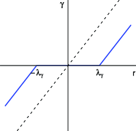
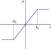
(a)	(b)
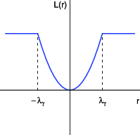
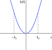
(c)	(d)

Figure 1: Modification of the squared error loss with a case-specific parameter. (a) $\gamma$ versus the residual $r$, (b) the adjusted residual $r^{*}$ versus the ordinary residual $r$, (c) a truncated squared error loss as the $\gamma$-adjusted loss and (d) the effective loss.

3.1 Least Squares Method

Taking the least squares method as a baseline modeling procedure $\mathcal{M}$, we make a link between its modification via case-specific parameters and a classical robust regression procedure.

The least squares estimator of $\beta=(\beta_{1},\ldots,\beta_{p})^{\top}$ is the minimizer $\hat{\beta}\in\mathbb{R}^{p}$ of $L(\beta)=\frac{1}{2}(Y-X\beta)^{\top}(Y-X\beta)$. To reduce the sensitivity of the estimator to influential observations, the $p$ covariates are augmented by $n$ case indicators. Let $z_{i}$ be the indicator variable taking 1 for the $i$th observation and 0 otherwise, and let $\underline{\gamma}=(\gamma_{1},\ldots,\gamma_{n})^{\top}$ be the coefficients of the case indicators. The additional design matrix $Z$ for $z_{i}$ is the identity matrix, and $Z\underline{\gamma}$ becomes $\underline{\gamma}$ itself. The proposed modification of the least squares method with $J_{2}(\underline{\gamma})=\|\underline{\gamma}\|_{1}=\sum_{i=1}^{n}|\gamma_{i}|$ leads to a well-known robust regression procedure. For the robust modification, we find $\hat{\beta}\in\mathbb{R}^{p}$ and $\hat{\underline{\gamma}}\in\mathbb{R}^{n}$ that minimize

$$\qquad L(\beta,\underline{\gamma}) = \tfrac{1}{2}\{Y-(X\beta+\underline{\gamma})\}^{\top}\{Y-(X\beta+\underline{\gamma})\}$$

$${}+\lambda_{\gamma}\|\underline{\gamma}\|_{1},$$

where $\lambda_{\gamma}$ is a fixed regularization parameter constraining $\underline{\gamma}$. Just as the ordinary LASSO with the $\ell_{1}$ norm penalty stabilizes regression coefficients byshrinkage and selection, the additional penalty in (3.1) has the same effect on $\underline{\gamma}$, whose components gauge the extent of case influences.

The minimizer $\hat{\underline{\gamma}}$ of $L(\hat{\beta},\underline{\gamma})$ for a fixed $\hat{\beta}$ can be found by soft-thresholding the residual vector $r=Y-X\hat{\beta}$. That is, $\hat{\gamma}_{i}=\operatorname{sgn}(r_{i})(|r_{i}|-\lambda_{\gamma})_{+}$. For observations with small residuals, $|r_{i}|\leq\lambda_{\gamma}$, $\hat{\gamma}_{i}$ is set equal to zero with no effect on the current fit, and for those with large residuals, $|r_{i}|>\lambda_{\gamma}$, $\hat{\gamma}_{i}$ is set equal to the residual $r_{i}=y_{i}-x_{i}^{\top}\hat{\beta}$ offset by $\lambda_{\gamma}$ toward zero. Combining $\hat{\underline{\gamma}}$ with $\hat{\beta}$, we define the adjusted residuals to be $r^{*}_{i}=y_{i}-x_{i}^{\top}\hat{\beta}-\hat{\gamma}_{i}$; that is, $r^{*}_{i}=r_{i}$ if $|r_{i}|\leq\lambda_{\gamma}$, and $r^{*}_{i}=\operatorname{sgn}(r_{i})\lambda_{\gamma}$, otherwise. Thus, introduction of the case-specific parameters along with the $\ell_{1}$ penalty on $\underline{\gamma}$ amounts to winsorizing the ordinary residuals. The $\gamma$-adjusted loss is equivalent to truncated squared error loss which is $(y-x^{\top}\beta)^{2}$ if $|y-x^{\top}\beta|\leq\lambda_{\gamma}$, and is $\lambda_{\gamma}^{2}$ otherwise. Figure 1 shows (a) the relationship between the ordinary residual $r$ and the corresponding $\gamma$, (b) the residual and the adjusted residual $r^{*}$, (c) the $\gamma$-adjusted loss as a function of $r$, and (d) the effective loss.

The effective loss is $\mathcal{L}_{\lambda_{\gamma}}(y,x^{\top}\beta)=(y-x^{\top}\beta)^{2}/2$ if $|y-x^{\top}\beta|\leq\lambda_{\gamma}$, and $\lambda_{\gamma}^{2}/2+\lambda_{\gamma}(|y-x^{\top}\beta|-\lambda_{\gamma})$ otherwise. This effective loss matches Huber’s loss function for robust regression ((Huber, 1981)). As in robust regression, we choose a sufficiently large $\lambda_{\gamma}$ so that only a modest fraction of the residuals are adjusted. Similarly, modification of the LASSO as a penalized regression procedure yields the Huberized LASSO described by Rosset and Zhu (2004).

3.2 Location Families

More generally, a wide class of problems can be cast in the form of a minimization of $L(\beta)=\break\sum_{i=1}^{n}g(y_{i}-x_{i}^{\top}\beta)$ where $g(\cdot)$ is the negative log-likelihood derived from a location family. The assumption that we have a location family implies that the negative log-likelihood is a function only of $r_{i}=y_{i}-x_{i}^{\top}\beta$. Dropping the subscript, common choices for the negative log-likelihood, $g(r)$, include $r^{2}$ (least squares, normal distributions) and $|r|$ (least absolute deviations, Laplace distributions).

Introducing the case-specific parameters $\gamma_{i}$, we wish to minimize

$$L(\beta,\underline{\gamma})=\sum_{i=1}^{n}g(y_{i}-x_{i}^{\top}\beta-\gamma_{i})+\lambda_{\gamma}\|\underline{\gamma}\|_{1}.$$

For minimization with a fixed $\hat{\beta}$, the next result applies to a broad class of $g(\cdot)$ (but not to $g(r)=|r|$).

Proposition 1

Suppose that $g$ is strictly convex with the minimum at 0, and $\lim_{r\rightarrow\pm\infty}g^{\prime}(r)=\pm\infty$, respectively. Then,

$$\hat{\gamma} = \operatorname{arg}\min_{\gamma\in\mathbb{R}}~{}g(r-\gamma)+\lambda_{\gamma}|\gamma|$$

$$= \cases{r-g^{\prime-1}(\lambda_{\gamma}),\vspace*{2pt}\cr\quad\hskip 11.0pt\mbox{for }r>g^{\prime-1}(\lambda_{\gamma}),\vspace*{2pt}\cr 0,\quad\mbox{for }g^{\prime-1}(-\lambda_{\gamma})\leq r\leq g^{\prime-1}(\lambda_{\gamma}),\vspace*{2pt}\cr r-g^{\prime-1}(-\lambda_{\gamma}),\vspace*{2pt}\cr\quad\hskip 11.0pt\mbox{for }r<g^{\prime-1}(-\lambda_{\gamma}).}$$

The proposition follows from straightforward algebra. Set the first derivative of the decoupled minimization equation equal to $0$ and solve for $\gamma$. Inserting these values for $\hat{\gamma}_{i}$ into the equation for $L(\beta,\underline{\gamma})$ yields

$$L(\hat{\beta},\hat{\underline{\gamma}})=\sum_{i=1}^{n}g(r_{i}-\hat{\gamma_{i}})+\lambda_{\gamma}\|\hat{\underline{\gamma}}\|_{1}.$$

The first term in the summation can be decomposed into three parts. Large $r_{i}$ contribute $g(r_{i}-r_{i}+g^{\prime-1}(\lambda_{\gamma}))=g(g^{\prime-1}(\lambda_{\gamma}))$. Large, negative $r_{i}$ contribute $g(g^{\prime-1}(-\lambda_{\gamma}))$. Those $r_{i}$ with intermediate values have $\hat{\gamma}_{i}=0$ and so contribute $g(r_{i})$. Thus a graphical depiction of the $\gamma$-adjusted loss is much like that in Figure 1, panel (c), where the loss is truncated above. For asymmetric distributions (and hence asymmetric log-likelihoods), the truncation point may differ for positive and negative residuals. It should be remembered that when $|r_{i}|$ is large, the corresponding $\hat{\gamma}_{i}$ is large, implying a large contribution of $\|\underline{\gamma}\|_{1}$ to the overall minimization problem. The residuals will tend to be large for vectors $\beta$ that are at odds with the data. Thus, in a sense, some of the loss which seems to disappear due to the effective truncation of $g$ is shifted into the penalty term for $\gamma$. Hence the effective loss $\mathcal{L}_{\lambda_{\gamma}}(y,f(x;\beta))=g(y-f(x;\beta)-\hat{\gamma})+\lambda_{\gamma}|\hat{\gamma}|$ is the same as the original loss, $g(y-f(x;\beta))$ when the residual is in $[g^{\prime-1}(-\lambda_{\gamma}),\break g^{\prime-1}(\lambda_{\gamma})]$ and is linear beyond the interval. The linearized part of $g$ is joined with $g$ such that $\mathcal{L}_{\lambda_{\gamma}}$ is differentiable.

Computationally, the minimization of $L(\beta,\hat{\underline{\gamma}})$ given $\hat{\underline{\gamma}}$ entails application of the same modeling procedure $\mathcal{M}$ with $g$ to winsorized pseudo responses $y^{*}_{i}=y_{i}-\hat{\gamma}_{i}$, where $y^{*}_{i}=y_{i}$ for $g^{\prime-1}(-\lambda_{\gamma})\leq r_{i}\leq g^{\prime-1}(\lambda_{\gamma})$, $y^{*}_{i}=g^{\prime-1}(\lambda_{\gamma})$ for $r>g^{\prime-1}(\lambda_{\gamma})$, and $y^{*}_{i}=g^{\prime-1}(-\lambda_{\gamma})$ for $r<g^{\prime-1}(-\lambda_{\gamma})$. So, the $\hat{\underline{\gamma}}$-adjusted data in Step 2 of the main algorithm consist of $(x_{i},y_{i}^{*})$ pairs in each iteration. A related idea of subsetting data and model-fitting to the subset iteratively for robustness can be found in the computer vision literature, the random sample consensus algorithm (Fischler and Bolles, 1981) for instance.

3.3 Quantile Regression

Consider median regression with absolute deviation loss $\mathcal{L}(y,x^{\top}\beta)=|y-x^{\top}\beta|$, which is not covered in the foregoing discussion. It can be verified easily that the $\ell_{1}$-adjustment of $\mathcal{L}$ is void due to the piecewise linearity of the loss, reaffirming the robustness of median regression. For an effectual adjustment, the $\ell_{2}$ norm regularization of the case-specific parameters is considered. With the case-specific parameters $\gamma_{i}$, we have the following objective function for modified median regression:

$$L(\beta,\underline{\gamma})=\sum_{i=1}^{n}|y_{i}-x_{i}^{\top}\beta-\gamma_{i}|+\frac{\lambda_{\gamma}}{2}\|\underline{\gamma}\|_{2}^{2}.$$ (3)

For a fixed $\hat{\beta}$ and residual $r=y-x^{\top}\hat{\beta}$, the $\hat{\gamma}$ minimizing $|r-\gamma|+\frac{\lambda_{\gamma}}{2}\gamma^{2}$ is given by

$$\operatorname{sgn}(r)\frac{1}{\lambda_{\gamma}}I\biggl{(}|r|>\frac{1}{\lambda_{\gamma}}\biggr{)}+rI\biggl{(}|r|\leq\frac{1}{\lambda_{\gamma}}\biggr{)}.$$

The $\gamma$-adjusted loss for median regression is

$$\mathcal{L}(y,x^{\top}\beta+\hat{\gamma})=\biggl{|}y-x^{\top}\beta-\frac{1}{\lambda_{\gamma}}\biggr{|}I\biggl{(}|y-x^{\top}\beta|>\frac{1}{\lambda_{\gamma}}\biggr{)},$$

as shown in Figure 3(a) below. Interestingly, this $\ell_{2}$-adjusted absolute deviation loss is the same as the so-called “$\varepsilon$-insensitive linear loss” for support vector regression ((Vapnik, 1998)) with $\varepsilon=1/\lambda_{\gamma}$.

With this adjustment, the effective loss is Huberized squared error loss. The $\ell_{2}$ adjustment makes median regression more efficient by rounding the sharp corner of the loss, and leads to a hybrid procedure which lies between mean and median regression. Note that, to achieve the desired effect for median regression, one chooses quite a different value of $\lambda_{\gamma}$ than one would when adjusting squared error loss for a robust mean regression.

The modified median regression procedure can be also combined with a penalty on $\beta$ for shrinkage and/or selection. Bi et al. (2003) considered support vector regression with the $\ell_{1}$ norm penalty $\|\beta\|_{1}$ for simultaneous robust regression and variable selection. These authors relied on the $\varepsilon$-insensitive linear loss which comes out as the $\gamma$-adjusted loss of the absolute deviation. In contrast, we rely on the effective loss which produces a different solution.

In general, quantile regression (Koenker and Bassett, 1978; (Koenker and Hallock, 2001)) can be used to estimate conditional quantiles of $y$ given $x$. It is a useful regression technique when the assumption of normality on the distribution of the errors $\varepsilon$ is not appropriate, for instance, when the error distribution is skewed or heavy-tailed. For the $q$th quantile, the check function $\rho_{q}$ is employed:

$$\rho_{q}(r)=\cases{qr,&$\mbox{for }r\geq 0,$\vspace*{2pt}\cr-(1-q)r,&$\mbox{for }r<0.$}$$ (4)

The standard procedure for the $q$th quantile regression finds $\beta$ that minimizes the sum of asymmetrically weighted absolute errors with weight $q$ on positive errors and weight $(1-q)$ on negative errors:

$$L(\beta)=\sum_{i=1}^{n}\rho_{q}(y_{i}-x_{i}^{\top}\beta).$$

Consider modification of $\rho_{q}$ with a case-specific parameter $\gamma$ and $\ell_{2}$ norm regularization. Due to the asymmetry in the loss, except for $q=1/2$, the size of reduction in the loss by the case-specific parameter $\gamma$ would depend on its sign. Given $\hat{\beta}$ and residual $r=y-x^{\top}\hat{\beta}$, if $r\geq 0$, then the positive $\gamma$ would lower $\rho_{q}$ by $q\gamma$, while if $r<0$, the negative $\gamma$ with the same absolute value would lower the loss by $(q-1)\gamma$. This asymmetric impact on the loss is undesirable. Instead, we create a penalty that leads to the same reduction in loss for positive and negative $\gamma$ of the same magnitude. In other words, the desired $\ell_{2}$ norm penalty needs to put $q\gamma_{+}$ and $(1-q)\gamma_{-}$ on an equal footing. This leads to the following penalty proportional to $q^{2}\gamma_{+}^{2}$ and $(1-q)^{2}\gamma_{-}^{2}$:

$$J_{2}(\gamma):=\{q/(1-q)\}\gamma_{+}^{2}+\{(1-q)/q\}\gamma_{-}^{2}.$$

When $q=1/2$, $J_{2}(\gamma)$ becomes the symmetric $\ell_{2}$ norm of $\gamma$.

With this asymmetric penalty, given $\hat{\beta}$, $\hat{\gamma}$ is now defined as

$$\operatorname{arg}\min_{\gamma\in\mathbb{R}}\mathcal{L}_{\lambda_{\gamma}}(\hat{\beta},\gamma):=\rho_{q}(r-\gamma)+\frac{\lambda_{\gamma}}{2}J_{2}(\gamma),$$ (5)

and is explicitly given by

$$-\frac{q}{\lambda_{\gamma}}I\biggl{(}r<-\frac{q}{\lambda_{\gamma}}\biggr{)}+rI\biggl{(}-\frac{q}{\lambda_{\gamma}}\leq r<\frac{1-q}{\lambda_{\gamma}}\biggr{)}$$

$$\quad{}+\frac{1-q}{\lambda_{\gamma}}I\biggl{(}r\geq\frac{1-q}{\lambda_{\gamma}}\biggr{)}.$$

The effective loss $\rho_{q}^{\gamma}$ is then given by

$$\rho_{q}^{\gamma}(r)=\cases{(q-1)r-\displaystyle\frac{q(1-q)}{2\lambda_{\gamma}},\vspace*{2pt}\cr\quad\mbox{for }r<-\displaystyle\frac{q}{\lambda_{\gamma}},\vspace*{2pt}\cr\displaystyle\frac{\lambda_{\gamma}}{2}\frac{1-q}{q}r^{2},\vspace*{2pt}\cr\quad\mbox{for }-\!\displaystyle\frac{q}{\lambda_{\gamma}}\leq r<0,\vspace*{2pt}\cr\displaystyle\frac{\lambda_{\gamma}}{2}\frac{q}{1-q}r^{2},\vspace*{2pt}\cr\quad\mbox{for }0\leq r<\displaystyle\frac{1-q}{\lambda_{\gamma}},\vspace*{2pt}\cr qr-\displaystyle\frac{q(1-q)}{2\lambda_{\gamma}},\vspace*{2pt}\cr\quad\mbox{for }r\geq\displaystyle\frac{1-q}{\lambda_{\gamma}},}$$ (6)

and its derivative is

$$\psi_{q}^{\gamma}(r)=\cases{q-1,&$\mbox{for }\displaystyle r<-\frac{q}{\lambda_{\gamma}},$\vspace*{2pt}\cr\displaystyle\lambda_{\gamma}\frac{1-q}{q}r,&$\mbox{for }\displaystyle-\!\frac{q}{\lambda_{\gamma}}\leq r<0,$\vspace*{2pt}\cr\displaystyle\lambda_{\gamma}\frac{q}{1-q}r,&$\mbox{for }0\leq r<\displaystyle\frac{1-q}{\lambda_{\gamma}},$\vspace*{2pt}\cr q,&$\mbox{for }r\geq\displaystyle\frac{1-q}{\lambda_{\gamma}}.$}$$ (7)

We note that, under the assumption that the density is locally constant in a neighborhood of the quantile, the quantile remains the $0$ of the effective $\psi_{q}^{\gamma}$ function.

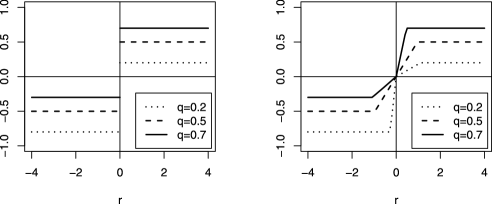
Figure 2: The derivative of the check loss in the left panel, $\psi_{q}$, and that of the modified check loss in the right panel, $\psi_{q}^{\gamma}$, for $q=0.2$, $0.5$ and $0.7$.

Figure 2 compares the derivative of the check loss with that of the effective loss in (6). Through penalization of a case-specific parameter, $\rho_{q}$ is modified to have a continuous derivative at the origin joined by two lines with a different slope that depends on $q$. The effective loss is reminiscent of the asymmetric squared error loss ($q(r_{+})^{2}+(1-q)(r_{-})^{2}$) considered by Newey and Powell (1987) and Efron (1991) for the so-called expectiles. The proposed modification of the check loss produces a hybrid of the check loss and asymmetric squared error loss, however, with different weights than those for expectiles, to estimate quantiles. The effective loss is formally similar to the rounded-corner check loss of Nychka et al. (1995) who used a vanishingly small adjustment to speed computation. Portnoy and Koenker (1997) thoroughly discussed efficient computation for quantile regression.

Redefining $J_{2}(\underline{\gamma})$ as the sum of the asymmetric penalty for the case-specific parameter $\gamma_{i}$, $i=1,\ldots,n$, modified quantile regression is formulated as a procedure that finds $\beta$ and $\underline{\gamma}$ by minimizing

$$\quad L(\beta,\underline{\gamma})=\sum_{i=1}^{n}\rho_{q}(y_{i}-x_{i}^{\top}\beta-\gamma_{i})+\frac{\lambda_{\gamma}}{2}J_{2}(\underline{\gamma}).$$ (8)

In extensive simulation studies (Jung, MacEachern and Lee, 2010), such adjustment of the standard quantile regression procedure generally led to more accurate estimates. See Section 5.1.1 for a summary of the studies. This is confirmed in theNHANES data analysis in Section 6.1.

For large enough samples, with a fixed $\lambda_{\gamma}$, the bias of the enhanced estimator will typically outweigh its benefits. The natural approach is to adjust the penalty attached to the case-specific covariates as the sample size increases. This can be accomplished by increasing the parameter $\lambda_{\gamma}$ as the sample size $n$ grows.

Let $\lambda_{\gamma}:=cn^{\alpha}$ for some constant $c$ and $\alpha>0$. The following theorem shows that if $\alpha$ is sufficiently large, the modified quantile regression estimator $\hat{\beta}_{n}^{\gamma}$, which minimizes $\sum_{i=1}^{n}\rho_{q}^{\gamma}(y_{i}-x_{i}^{\top}\beta)$ or equivalently (8), is asymptotically equivalent to the standard estimator $\hat{\beta}_{n}$. Knight (1998) proved the asymptotic normality of the regression quantile estimator $\hat{\beta}_{n}$ under some mild regularity conditions. Using the arguments in Koenker (2005), we show that $\hat{\beta}_{n}^{\gamma}$ has the same limiting distribution as $\hat{\beta}_{n}$, and thus it is $\sqrt{n}$-consistent if $\alpha$ is sufficiently large.

Allowing a potentially different error distribution for each observation, let $Y_{1},Y_{2},\ldots$ be independent random variables with c.d.f.’s $F_{1},F_{2},\ldots$ and suppose that each $F_{i}$ has continuous p.d.f. $f_{i}$. Assume that the $q$th conditional quantile function of $Y$ given $x$ is linear in $x$ and given by $x^{\top}\beta(q)$, and let $\xi_{i}(q):=x_{i}^{\top}\beta(q)$. Now consider the following regularity conditions:

1. [(C-1)]

2. $f_{i}(\xi)$, $i=1,2,\ldots,$ are uniformly bounded away from 0 and $\infty$ at $\xi_{i}$.

3. $f_{i}(\xi)$, $i=1,2,\ldots,$ admit a first-order Taylor expansion at $\xi_{i}$, and $f^{\prime}_{i}(\xi)$ are uniformly bounded at $\xi_{i}$.

4. There exists a positive definite matrix $D_{0}$ such that $\lim_{n\rightarrow\infty}n^{-1}\sum x_{i}x_{i}^{\top}=D_{0}$.

5. There exists a positive definite matrix $D_{1}$ such that $\lim_{n\rightarrow\infty}n^{-1}\sum f_{i}(\xi_{i})x_{i}x_{i}^{\top}=D_{1}$.

6. $\max_{i=1,\ldots,n}\|x_{i}\|/\sqrt{n}\rightarrow 0$ in probability.

(C-1) and (C-3) through (C-5) are the conditions considered for the limiting distribution of the standard regression quantile estimator $\hat{\beta}_{n}$ in Koenker (2005) while (C-2) is an additional assumption that we make.

Theorem 2

Under the conditions (C-1)–(C-5), if $\alpha>1/3$, then

$$\sqrt{n}\bigl{(}\hat{\beta}^{\gamma}_{n}-\beta(q)\bigr{)}\stackrel{{\scriptstyle d}}{{\rightarrow}}N\bigl{(}0,q(1-q)D_{1}^{-1}D_{0}D_{1}^{-1}\bigr{)}.$$

The proof of the theorem is in the Appendix.

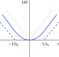
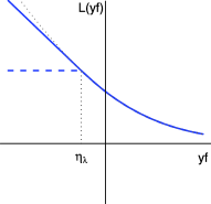
(a)	(b)	(c)

Figure 3: Modification of (a) absolute deviation loss for median regression with $\ell_{2}$ penalty, (b) negative log-likelihood for logistic regression with $\ell_{1}$ penalty, and (c) hinge loss for the support vector machine with $\ell_{2}$ penalty. The solid lines are for the effective loss, the dashed lines are for the $\gamma$-adjusted loss, and the dotted lines are for the original loss in each panel.

4 Classification

Now suppose that $y_{i}$’s indicate binary outcomes. For modeling and prediction of the binary responses, we mainly consider margin-based procedures such as logistic regression, support vector machines ((Vapnik, 1998)), and boosting ((Freund and Schapire, 1997)). These procedures can be modified by the addition of case indicators.

4.1 Logistic Regression

Although it is customary to label a binary outcome as 0 or 1 in logistic regression, we instead adopt the symmetric labels of $\{-1,1\}$ for $y_{i}$’s. The symmetry facilitates comparison of different classification procedures. Logistic regression takes the negative log-likelihood as a loss for estimation of logit $f(x)=\log[p(x)/(1-p(x))]$. The loss, $\mathcal{L}(y,f(x))=\log[1+\exp(-yf(x))]$, can be viewed as a function of the so-called margin, $yf(x)$. This functional margin of $yf(x)$ is a pivotal quantity for defining a family of loss functions in classification similar to the residual in regression.

As in regression with continuous responses, case indicators can be used to modify the logit function $f(x)$ in logistic regression to minimize

$$L(\beta_{0},\beta,\underline{\gamma})$$

$$\quad=\sum_{i=1}^{n}\log\bigl{(}1+\exp\bigl{(}-y_{i}\{f(x_{i};\beta_{0},\beta)+\gamma_{i}\}\bigr{)}\bigr{)}$$ (9)

$$\qquad{}+\lambda_{\gamma}\|\underline{\gamma}\|_{1},$$

where $f(x;\beta_{0},\beta)=\beta_{0}+x^{\top}\beta$. When it is clear in context, $f(x)$ will be used as abbreviated notation for $f(x;\beta_{0},\beta)$, a discriminant function, and the subscript $i$ will be dropped. For fixed $\hat{\beta}_{0}$ and $\hat{\beta}$, the minimization decouples, and $\gamma_{i}$ is determined by minimizing

$$\log\bigl{(}1+\exp\bigl{(}-y_{i}\{f(x_{i};\hat{\beta}_{0},\hat{\beta})+\gamma_{i}\}\bigr{)}\bigr{)}+\lambda_{\gamma}|\gamma_{i}|.$$

First note that the minimizer $\gamma_{i}$ must have the same sign as $y_{i}$. Letting $\tau=yf(x)$ and assuming that $0<\lambda_{\gamma}<1$, we have $\arg\min_{\gamma\geq 0}\log(1+\exp(-\tau-\gamma))+\lambda_{\gamma}|\gamma|=\log\{(1-\lambda_{\gamma})/\lambda_{\gamma}\}-\tau$ if $\tau\leq\log\{(1-\lambda_{\gamma})/\lambda_{\gamma}\}$, and 0 otherwise. This yields a truncated negative log-likelihood given by

$$\mathcal{L}(y,f(x))=\cases{\log\bigl{(}1+\lambda_{\gamma}/(1-\lambda_{\gamma})\bigr{)},\vspace*{2pt}\cr\quad\mbox{if }yf(x)\leq\log\{(1-\lambda_{\gamma})/\lambda_{\gamma}\},\vspace*{2pt}\cr\log\bigl{(}1+\exp(-yf(x))\bigr{)},\vspace*{2pt}\cr\quad\mbox{otherwise,}}$$

as the $\gamma$-adjusted loss. This adjustment is reminiscent of Pregibon’s (1982) proposal tapering the deviance function so as to downweight extreme observations, thereby producing a robust logistic regression. See Figure 3(b) for the $\gamma$-adjusted loss (the dashed line), where $\eta_{\lambda}:=\log\{(1-\lambda_{\gamma})/\lambda_{\gamma}\}$ is a decreasing function of $\lambda_{\gamma}$. $\lambda_{\gamma}$ determines the level of truncation of the loss. As $\lambda_{\gamma}$ tends to $1$, there is no truncation. Figure 3(b) also shows the effective loss (the solid line) for the $\ell_{1}$ adjustment, which linearizes the negative log-likelihood below $\eta_{\lambda}$.

4.2 Large Margin Classifiers

With the symmetric class labels, the foregoing characterization of the case-specific parameter $\gamma$ in logistic regression can be easily generalized to various margin-based classification procedures. In classification, potential outliers are those cases with large negative margins. Let $g(\tau)$ be a loss function of the margin $\tau=yf(x)$. The following proposition, analogous to Proposition 1, holds for a general family of loss functions.

Proposition 3

Suppose that $g$ is convex and monotonically decreasing in $\tau$, and $g^{\prime}$ is continuous. Then, for $\lambda_{\gamma}<-\lim_{\tau\rightarrow-\infty}g^{\prime}(\tau)$,

$$\hat{\gamma} = \arg\min_{\gamma\in\mathbb{R}}~{}g(\tau+\gamma)+\lambda_{\gamma}|\gamma|$$

$$= \cases{g^{\prime-1}(-\lambda_{\gamma})-\tau,&$\mbox{for }\tau\leq g^{\prime-1}(-\lambda_{\gamma}),$\vspace*{2pt}\cr 0,&$\mbox{for }\tau>g^{\prime-1}(-\lambda_{\gamma}).$}$$

The proof is straightforward. Examples of the margin-based loss $g$ satisfying the assumption include the exponential loss $g(\tau)=\exp(-\tau)$ in boosting, the squared hinge loss $g(\tau)=\{(1-\tau)_{+}\}^{2}$ in the support vector machine ((Lee and Mangasarian, 2001)), and the negative log-likelihood $g(\tau)=\log(1+\exp(-\tau))$ in logistic regression. Although their theoretical targets are different, all of these loss functions are truncated above for large negative margins when adjusted by $\gamma$. Thus, the effective loss $\mathcal{L}_{\lambda_{\gamma}}(y,f(x))=g(yf(x)+\hat{\gamma})+\lambda_{\gamma}|\hat{\gamma}|$ is obtained by linearizing $g$ for $yf(x)<g^{\prime-1}(-\lambda_{\gamma})$.

The effect of $\hat{\gamma}$-adjustment depends on the form of $g$, and hence on the classification method. For boosting, $\hat{\gamma}\!=\!-\log\lambda_{\gamma}-yf(x)$ if $yf(x)\!\leq\!-\log\lambda_{\gamma}$, and is 0 otherwise. This gives $L(\beta_{0},\beta,\hat{\underline{\gamma}})\!=\!\sum_{i=1}^{n}\exp(-y_{i}\cdot f(x_{i};\beta_{0},\beta)-\hat{\gamma}_{i})\!=\!\sum_{i=1}^{n}\exp({-}\hat{\gamma}_{i})\exp({-}y_{i}f(x_{i};\beta_{0},\beta)\!)$. So, finding $\beta_{0}$ and $\beta$ given $\hat{\underline{\gamma}}$ amounts to weighted boosting, where the positive case-specific parameters $\hat{\gamma}_{i}$ downweight the corresponding cases by$\exp(-\hat{\gamma}_{i})$. For the squared hinge loss in the support vector machine, $\hat{\gamma}=1-yf(x)-\lambda_{\gamma}/2$ if $yf(x)\leq 1-\lambda_{\gamma}/2$, and is $0$ otherwise. A positive case-specific parameter $\hat{\gamma}_{i}$ has the effect of relaxing the margin requirement, that is, lowering the joint of the hinge for that specific case. This allows the associated slack variable to be smaller in the primal formulation. Accordingly, the adjustment affects the coefficient of the linear term in the dual formulation of the quadratic programming problem.

As a related approach to robust classification, Wu and Liu (2007) proposed truncation of margin-based loss functions and studied theoretical properties that ensure classification consistency. Similarity exists between our proposed adjustment of a loss function with $\gamma$ and truncation of the loss at some point. However, it is the linearization of a margin-based loss function on the negative side that produces its effective loss, and minimization of the effective loss is quite different from minimization of the truncated (i.e., adjusted) loss. Linearization is more conducive to computation than is truncation. Application of the result in Bartlett, Jordan and McAuliffe (2006) shows that the linearized loss functions satisfy sufficient conditions for classification consistency, namely Fisher consistency, which is the main property investigated by Wu and Liu (2007) for truncated loss functions.

Xu, Caramanis and Mannor (2009) showed that regularization in the standard support vector machine is equivalent to a robust formulation under disturbances of $x$ without penalty. In contrast, under our approach, robustness of classification methods is considered through the margin, which is analogous to the residual in regression. This formulation can cover outliers due to perturbation in $x$ as well as mislabeling of $y$.

4.3 Support Vector Machines

As a special case of a large margin classifier, the linear support vector machine (SVM) looks for the optimal hyperplane $f(x;\beta_{0},\beta)=\beta_{0}+x^{\top}\beta=0$ minimizing

$$\hskip 19.0ptL_{\lambda}(\beta_{0},\beta)=\sum_{i=1}^{n}[1-y_{i}f(x_{i};\beta_{0},\beta)]_{+}+\frac{\lambda}{2}\|\beta\|_{2}^{2},$$ (10)

where $[t]_{+}=\max(t,0)$ and $\lambda>0$ is a regularization parameter. Since the hinge loss for the SVM, $g(\tau)=(1-\tau)_{+}$, is piecewise linear, its linearization with $\|\underline{\gamma}\|_{1}$ is void, indicating that it has little need of further robustification. Instead, we consider modification of the hinge loss with $\|\underline{\gamma}\|_{2}^{2}$. This modification is expected to improve efficiency, as in quantile regression.

Using the case indicators $z_{i}$ and their coefficients $\gamma_{i}$, we modify (10), arriving at the problem of minimizing

$$L(\beta_{0},\beta,\underline{\gamma}) = \sum_{i=1}^{n}[1-y_{i}\{f(x_{i};\beta_{0},\beta)+\gamma_{i}\}]_{+}$$

$${}+\frac{\lambda_{\beta}}{2}\|\beta\|_{2}^{2}+\frac{\lambda_{\gamma}}{2}\|\underline{\gamma}\|_{2}^{2}.$$

For fixed $\hat{\beta}_{0}$ and $\hat{\beta}$, the minimizer $\hat{\underline{\gamma}}$ of $L(\hat{\beta}_{0},\hat{\beta},\underline{\gamma})$ is obtained by solving the decoupled optimization problem of

$$\min_{\gamma_{i}\in\mathbb{R}}[1-y_{i}f(x_{i};\hat{\beta}_{0},\hat{\beta})-y_{i}\gamma_{i}]_{+}+\frac{\lambda_{\gamma}}{2}\gamma_{i}^{2}\quad\mbox{for each }\gamma_{i}.$$

With an argument similar to that for logistic regression, the minimizer $\hat{\gamma}_{i}$ should have the same sign as $y_{i}$. Let $\xi\!=\!1-yf$. A simple calculation shows that

$$\arg\min_{\gamma\geq 0}[\xi-\gamma]_{+}+\frac{\lambda_{\gamma}}{2}\gamma^{2}$$

$$\quad=\cases{0,&$\mbox{if }\xi\leq 0,$\vspace*{2pt}\cr\xi,&$\mbox{if }0<\xi<1/\lambda_{\gamma},$\vspace*{2pt}\cr 1/\lambda_{\gamma},&$\mbox{if }\xi\geq 1/\lambda_{\gamma}.$}$$

Hence, the increase in margin $y_{i}\hat{\gamma}_{i}$ due to inclusion of $\gamma$ is given by

$$\{1-y_{i}f(x_{i})\}I\biggl{(}0<1-y_{i}f(x_{i})<\frac{1}{\lambda_{\gamma}}\biggr{)}$$

$$\quad{}+\frac{1}{\lambda_{\gamma}}I\biggl{(}1-y_{i}f(x_{i})\geq\frac{1}{\lambda_{\gamma}}\biggr{)}.$$

The $\gamma$-adjusted hinge loss is $\mathcal{L}(y,f(x))=[1-1/\lambda_{\gamma}-yf(x)]_{+}$ with the hinge lowered by $1/\lambda_{\gamma}$ as shown in Figure 3(c) (the dashed line). The effective loss (the solid line in the figure) is then given by a smooth function with the joint replaced with a quadratic piece between $1-1/\lambda_{\gamma}$ and 1 and linear beyond the interval.

5 Simulation Studies

We present results from various numerical experiments to illustrate the effect of the proposed modification of modeling procedures by regularization of case-specific parameters.

5.1 Regression

5.1.1 $\ell_{2}$-adjusted quantile regression

The effectiveness of the $\ell_{2}$-adjusted quantile regression depends on the penalty parameter $\lambda_{\gamma}$ in (6), which yields $(-q/\lambda_{\gamma},(1-q)/\lambda_{\gamma})$ as the interval of quadratic adjustment.

We undertook extensive simulation studies (available in (Jung, MacEachern and Lee, 2010)) to establish guidelines for selection of the penalty parameter $\lambda_{\gamma}$ in the linear regression model setting. The studies encompassed a range of sample sizes, from $10^{2}$ to $10^{4}$, a variety of quantiles, from $0.1$ to $0.9$, and distributions exhibiting symmetry, varying degrees of asymmetry, and a variety of tail behaviors. The modified quantile regression method was directly implemented by specifying the effective $\psi$-function $\psi_{q}^{\gamma}$, the derivative of the effective loss, in the rlm function in the R package.

An empirical rule was established via a (robust) regression analysis. The analysis considered $\lambda_{\gamma}$ of the form $c_{q}n^{\alpha}/\hat{\sigma}$, where $c_{q}$ is a constant depending on $q$ and $\hat{\sigma}$ is a robust estimate of the scale of the error distribution. The goal of the analysis was to find $\lambda_{\gamma}$ which, across a broad range of conditions, resulted in an MSE near the condition-specific minimum MSE. Here MSE is defined as mean squared error of estimated regression quantiles at a new $X$ integrated over the distribution of the covariates.

After initial examination of the MSE with a range of $\alpha$ values, we made a decision to set $\alpha$ to $0.3$ for good finite sample performance across a wide range of conditions. With fixed $\alpha$, we varied $c_{q}$ to obtain the smallest MSE by grid search for each condition under consideration. For a quick illustration, Figure 4 shows the intervals of adjustment with such optimal $c_{q}$ for various error distributions, $q$ values, and sample sizes. Wider optimal intervals indicate that more quadratic adjustment is preferred to the standard quantile regression for reduction of MSE. Clearly, Figure 4 demonstrates the benefit of the proposed quadratic adjustment of quantile regression in terms of MSE across a broad range of situations, especially when the sample size is small.

In general, MSE values begin to decrease as the size of adjustment increases from zero and increase after hitting the minimum, due to an increase in bias. There is an exception of this typical pattern when estimating the median with normally distributed errors. MSE monotonically decreases in this case as the interval of adjustment widens, confirming the optimality properties of least squares regression for normal theory regression. The comparisons between sample mean and sample median can be explicitly found under the $t$ error distributions using different degrees of freedom. The benefit of the median relative to the mean is greater for thicker tailed distributions. We observe that this qualitative behavior carries over to the optimal intervals. Thicker tails lead to shorter optimal intervals, as shown in Figure 4.

Modeling the optimal condition-specific $c_{q}$ as a function of $q$ through a robust regression analysis led to the rule, with $\alpha=0.30$, of $c_{q}\approx 0.5\exp(-2.118-1.097q)$ for $q<0.5$ and $c_{q}\approx 0.5\exp(-2.118-1.097(1-q))$ for $q\geq 0.5$. The simulation studies show that this choice of penalty parameter results in an accurate estimator of the quantile surface.

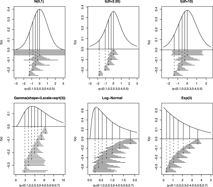
Figure 4: “Optimal” intervals of adjustment for different quantiles ($q$), sample sizes ($n$), and error distributions. The intervals range from the quantile minus $q/\lambda_{\gamma}$ to the quantile plus $(1-q)/\lambda_{\gamma}$, with $\lambda_{\gamma}$ minimizing MSE. The vertical lines in each distribution indicate the true quantiles. The stacked horizontal lines for each quantile are corresponding optimal intervals. Five intervals at each quantile are for $n=10^{2}$, $10^{2.5}$, $10^{3}$, $10^{3.5}$ and $10^{4}$, respectively, from the bottom.

Table 1: Distribution of difference in the number of selected variables for the fitted model to contaminated data from that to clean data

	LARS							Robust LARS
2-8,10-16Scenario	$\bolds{-3}$	$\bolds{-2}$	$\bolds{-1}$	0	1	2	3	$\bolds{-3}$	$\bolds{-2}$	$\bolds{-1}$	0	1	2	3
$\varepsilon$ contamination
Sparse	5*	06	21	48	13	5	02*	1*	4	12	71	07	05	0
Intermediate	5*	10	14	46	21	3	1	1*	3	14	64	14	04	0
Dense	2*	01	16	80	01	0	0	0*	0	08	89	03	00	0
$X$ contamination
Sparse	7*	05	15	34	20	7	12*	5*	3	16	36	22	12	6
Intermediate	1*	05	13	55	21	3	2	1*	3	18	50	23	04	1
Dense	0*	00	05	93	02	0	0	0*	0	04	94	02	00	0

[]Note: The entries with * are the cumulative counts of the specified case and more extreme cases.

5.1.2 Robust LASSO

We investigated the sensitivity of the LASSO (or LARS) and its robust version (obtained by the proposed $\ell_{1}$ modification) to contamination of the data through simulation.

For the robust LASSO, the iterative algorithm in Section 2 was implemented by using LARS (Efron et al., 2004a) as the baseline modeling procedure and winsorizing the residuals with $\lambda_{\gamma}$ as a bending constant. The bending constant was taken to be scale invariant, so that $\lambda_{\gamma}=k\hat{\sigma}$, where $k$ is a constant and $\hat{\sigma}$ is a robust scale estimate. The standard robust statistics literature ((Huber, 1981)) suggests that good choices of $k$ lie in the range from $1$ to $2$.

For brevity, we report only that portion of the results pertaining to accuracy of the fitted regression surface and inclusion of variates in the model when $k=2$. Similar results were obtained for $k$ near $2$. The results differ for extreme values of $k$. Throughout the simulation, the standard linear model $y=x^{\top}\beta+\varepsilon$ was assumed. Following the simulation setting in Tibshirani (1996), we generated $x=(x_{1},\ldots,x_{8})^{\top}$ from a multivariate normal distribution with mean zero and standard deviation 1. The correlation between $x_{i}$ and $x_{j}$ was set to $\rho^{|i-j|}$ with $\rho=0.5$. Three scenarios were considered with a varying degree of sparsity in terms of the number of nonzero true coefficients: (i) sparse: $\beta=(5,0,0,0,0,0,0,0)$, (ii) intermediate: $\beta=(3,1.5,0,0,2,0,0,0)$ and (iii) dense: $\beta_{j}=0.85$ for all $j=1,\ldots,8$. In all cases, the sample size was $100$. For the base case, $\varepsilon_{i}$ was assumed to follow $N(0,\sigma^{2})$ with $\sigma=3$. For potential outliers in $\varepsilon$, the first 5% of the $\varepsilon_{i}$’s were tripled, yielding a data set with more outliers. We also investigated sensitivity to high leverage cases. For this setting, we tripled the first 5% of the values of $x_{1}$. Thus the replicates were blocked across the three settings. The $C_{p}$ criterion was used to select the model.

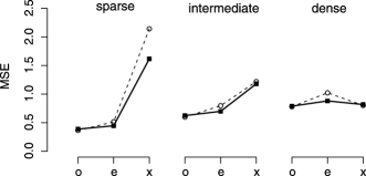
Figure 5: Mean squared error (MSE) of $\hat{\beta}$ for LARS and its robust version under three different scenarios in the simulation study. In each scenario, o, e, and x indicate clean data, data with contaminated measurement errors, and data with mismeasured first covariate. The dotted lines are for LARS while the solid lines are for robust LARS. The points are the average MSE for 100 replicates.

Figure 5 shows mean squared error (MSE) between the fitted and true regression surfaces, omitting intercepts. MSE is integrated across the distribution of a future $X$, taken to be that for the base case of the simulation. Over the $m=100$ replicates in the simulation, $\operatorname{MSE}=m^{-1}\sum_{i=1}^{m}(\hat{\beta}^{i}-\beta)^{\top}\Sigma(\hat{\beta}^{i}-\beta)$, where $\hat{\beta}^{i}$ is the estimate of $\beta$ for the $i$th replicate, and $\Sigma$ is the covariance matrix of $X$. LARS and robust LARS perform comparably in the base case, with the MSE for robust LARS being greater by $1$ to $6$ percent. For both LARS and robust LARS, MSE in the base case increases as one moves from the sparse to the dense scenario. MSE increases noticeably when $\varepsilon$ is contaminated, by a factor of $1.31$ to $1.41$ for LARS. For robust LARS, the factor for increase over the base case with LARS is $1.12$ to $1.22$. For contamination in $X$, results under LARS and robust LARS are similar in the intermediate and dense cases, with increases in MSE over the base case. For the sparse case, the coefficient of the contaminated covariate, $x_{1}$, is large relative to the other covariates. Here, robust LARS performs noticeably better than LARS, with a smaller increase in MSE.

Table 1 presents results on the difference in number of selected variables for pairs of models. In each pair, a contaminated model is contrasted with the corresponding uncontaminated model. The top half of the table presents results for contamination of $\varepsilon$. The distribution of the differences in the number of selected variables for the pairs of fitted models has a mode at $0$ in each scenario for both LARS and robust LARS. There is, however, substantial spread around $0$. The fitted models for the data with contaminated errors tend to have fewer variables than those for the original data, especially in the dense scenario. This may well be attributed to inflated estimates of $\sigma^{2}$ used in $C_{p}$ for the contaminated data, favoring relatively smaller models. The effect is stronger for LARS than for robust LARS, in keeping with the lessened impact of outliers on the robust estimate of $\sigma^{2}$.

The bottom half of Table 1 presents results for contamination of $X$. Again, the distributions of differences in model size have modes at $0$ in all scenarios. The distributions have substantial spread around $0$. Under the sparse scenario in which the contamination has a substantial impact on MSE, the distribution under robust LARS is more concentrated than under LARS.

The simulation demonstrates that the proposed robustification is successful in dealing with both contaminated errors and contaminated covariates. As expected, in contrast to LARS, robust LARS is effective in identifying observations with large measurement errors and lessening their influence. It is also effective at reducing the impact of high leverage cases, especially when the high leverage arises from a covariate with a large regression coefficient. The combined benefits of robustness to outliers and high leverage cases render robust LARS effective at dealing with influential cases in an automated fashion.

5.2 Classification

A three-part simulation study was carried out to examine the effect of the proposed modification of loss functions for classification. The primary focus is on (i) the efficiency of the modified SVM relative to the SVM with hinge loss and its smoothed version with quadratically modified hinge loss, and (ii) the robustness of logistic regression relative to modified logistic regression (via the linearized deviance). The secondary focus is on ensuring that robustness does not significantly degrade as efficiency is improved, and that efficiency does not suffer too much as robustness is improved.

All three parts of the simulation begin with $n=100$ cases generated from a pair of five-dimensional multivariate normal distributions, with identical covariance matrices and equal proportions for two classes ($y=\pm 1$). Without loss of generality, the covariance matrices were taken to be the identity. For the first part of the simulation, the separation between the two classes is fixed. The separation is determined by the difference in means of the multivariate normals, which, in turn, determine the Bayes error rate for the underlying problem. Throughout, once a method was fit to the data (i.e., a discriminant function was obtained), the error rate was calculated analytically. Each part of the simulation consisted of $400$ replicates.

Six methods were considered in this study: LDA (linear discriminant analysis) as a baseline method for the normal setting, the standard SVM, its variant with squared hinge loss (called Smooth SVM in (Lee and Mangasarian, 2001)), another variant with quadratically modified hinge loss (referred to as Huberized SVM in (Rosset and Zhu, 2007)), logistic regression, and the method with linearized binomial deviance (referred to as linearized LR in this study). The Huberized SVM and linearized LR were implemented through the fast Newton–Armijo algorithm proposed for Smooth SVM in Lee and Mangasarian (2001). To focus on the effect of the loss functions on the classification error rate, no penalty was imposed on the parameters of discriminant functions.

For the first part of the study, the mean vectors were set with a difference of 2.7 in the first coordinate and 0 elsewhere, yielding a Bayes error rate of 8.851%. Figure 6 compares the SVM and its variants in terms of the average excess error from the Bayes error rate. The $k$ on the $x$-axis corresponds to the bending constant, $1-1/\lambda_{\gamma}$ in the Huberized SVM. When $k$ is as small as $-1$, we see that quadratic modification in the Huberized SVM effectively yields the same result as Smooth SVM. As $k$ tends to 1, the Huberized SVM becomes the standard SVM. Clearly, there is a range of $k$ values for which the mean error rate of the Huberized SVM is lower than that of the standard SVM, demonstrating improved efficiency in classification. In fact, the improved efficiency of smooth versions of the hinge loss in the normal setting can be verified theoretically for large sample cases, where the relative efficiency is defined as the ratio of mean excess errors. See Lee and Wang (2011) for details.

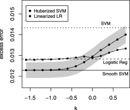
Figure 6: Mean excess error of the SVM variant with quadratically modified hinge loss (Huberized SVM) and the method with linearized deviance loss (linearized LR) as the bending constant $k$ varies. The gray band indicates a one standard error bound around the mean estimate for Huberized SVM from 400 replicates. The standard error for comparison of the Huberized SVM to another method varies, but is considerably smaller, due to the simulation design. The horizontal lines from top to bottom are for SVM, logistic regression and Smooth SVM, respectively.

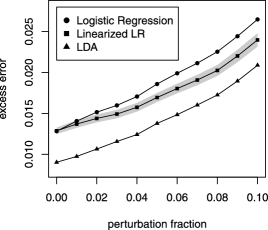
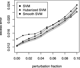
(a)	(b)

Figure 7: Mean excess errors of (a) logistic regression and linearized LR, and (b) SVM and its variants, as the proportion of perturbation varies. The gray band indicates a one standard error bound around the mean estimate for (a) linearized LR and (b) Huberized SVM from 400 replicates. The standard errors for comparisons are considerably smaller than indicated by the bands.

Figure 6 also displays a comparison between logistic regression and the linearized LR of Section 4, with bending constant $k=\log\{(1-\lambda_{\gamma})/\lambda_{\gamma}\}$. There is no appreciable difference in the excess error between logistic regression and its linearized version for negative values of $k$. Enhancing the robustness of logistic regression (shown in part two of the study) sacrifices almost none of its efficiency.

The value of the bending constant $k$ leading to the minimum error rate depends on the underlying problem itself, and the range of best $k$ values may differ for the Huberized SVM and linearized LR. The results in Figure 6 suggest that values of $k$ ranging from $-1$ to $0$ yield excellent performance for both procedures in this setting.

The second part of the study focuses on robustness. To study this, we perturbed each sample by flipping the class labels of a certain proportion of cases selected at random, and applied the six procedures to the perturbed sample. The estimated discriminant rules were evaluated in the same way as in the setting without perturbation.

Figure 7(a) highlights increased robustness of linearized LR (with $k=-0.5$) compared to logistic regression when some fraction of labels are flipped. As the proportion of mislabeled data increases, excess error rises for all of the procedures, including the baseline method of LDA. However, the rate of increase in error is slower for the modified logistic regression, as the linearized deviance dampens the influence of mislabeled cases on the discriminant rule.

Comparison of the SVM and its variants in the same setting reveals a trade-off between efficiency and robustness. Figure 7(b) shows that the squared hinge loss yields a lower error rate than hinge loss when the perturbation fraction is less than 6%. The trend is reversed when the fraction is higher than 6%. This trade-off is reminiscent of that between the sample mean and median as location parameter estimators. The Huberized SVM (with $k=-0.5$) as a hybrid method strikes a balance between the two. We note that the robustness of the SVM, compared with its variants, is more visible when two classes have less overlap (not shown here).

Table 2: Mean error rates of classification methods under various settings of mean difference and perturbation fraction. The lowest error rates are in bold when compared among the methods of the same type (either SVM or LR) for each scenario

		Huberized SVM			Linearized LR
3-4,6-7 Scenario	SVM	$\bolds{k=-0.5}$	$\bolds{k=-1}$	Smooth SVM	$\bolds{k=-0.5}$	$\bolds{k=-1}$	LR
Easy	0.0385	0.0376	0.0376	0.0376	0.0362	0.0363	0.0363
Intermediate	0.1028	0.1009	0.1008	0.1008	0.1014	0.1013	0.1013
Hard	0.1753	0.1727	0.1726	0.1726	0.1730	0.1729	0.1728
Easy${}+{}$5% flip	0.0348	0.0362	0.0371	0.0372	0.0383	0.0395	0.0411
Intermediate${}+{}$5% flip	0.1063	0.1050	0.1057	0.1059	0.1054	0.1061	0.1071
Hard${}+{}$5% flip	0.1790	0.1769	0.1773	0.1774	0.1772	0.1773	0.1778
Easy${}+{}$10% flip	0.0370	0.0415	0.0423	0.0421	0.0445	0.0465	0.0481
Intermediate${}+{}$10% flip	0.1107	0.1117	0.1127	0.1127	0.1125	0.1136	0.1150
Hard${}+{}$10% flip	0.1846	0.1833	0.1839	0.1840	0.1836	0.1841	0.1848

The third part of the study provides a comprehensive comparison of the methods. Three scenarios with differing degree of difficulty were considered; “easy,” “intermediate” and “hard” settings refer to the multivariate normal setting with the Bayes error rates of 2.275%, 8.851% and 15.866%, respectively. In addition, for scenarios with mislabeled cases, 5% and 10% of labels were flipped under each of the three settings. Two values of the bending constant ($k=-0.5$ and $-1$) were used for the Huberized SVM and the linearized LR. The results of comparison under nine scenarios are summarized in Table 2. The tabulated values are the mean error rates of the discriminant rules under each method.

When there are no mislabeled cases, the smooth variants of the SVM improve upon the performance of the standard SVM. As the separation between classes increases, the reduction in error due to modification of the hinge loss with fixed $k$ diminishes. Linearization of deviance in logistic regression does not appear to affect the error rate. In contrast, when there are mislabeled cases, linearization of the deviance renders logistic regression more robust across all the scenarios with differing class separations. Similarly, the standard SVM is less sensitive to mislabeling than its smooth variants. This makes the SVM more preferable as the proportion of mislabeled cases increases. However, in the difficult problem of little class separation, the quadratic modification in the Huberized SVM performs better than the SVM.

6 Applications

6.1 Analysis of the NHANES Data

We numerically compare standard quantile regression with modified quantile regression for analysis of real data. The Centers for Disease Control and Prevention conduct the National Health and Nutrition Examination Survey (NHANES), a large-scale survey designed to monitor the health and nutrition of residents of the United States. Many are concerned about the record levels of obesity in the population, and the survey contains information on height and weight of individuals, in addition to a variety of dietary and health-related questions. Obesity is defined through body mass index (BMI) in $\mathrm{kg}/\mathrm{m}^{2}$, a measure which adjusts weight for height. In this analysis, we describe the relationship between height and BMI among the $5938$ males over the age of $18$ in the aggregated NHANES data sets from 1999, 2001, 2003 and 2005. Our analyses do not adjust for NHANES’ complex survey design. In particular, no adjustment has been made for oversampling of selected groups or nonresponse. Since BMI is weight adjusted for height, the null expectation is that BMI and height are unrelated.

We fit a nonparametric quantile regression model to the data. The model is a six-knot regression spline using the natural basis expansion. The knots (held constant across quantiles) were chosen by eye. The rule for selection of the penalty parameter $\lambda_{\gamma}$ described in Section 5.1.1 was used for the NHANES data analysis.

Figure 8 displays the fits from standard (QR) and modified (QR.M) quantile regressions for the quantiles between $0.1$ and $0.9$ in steps of $0.05$. The fitted curves show a slight upward trend, some curvature overall, and mildly increasing spread as height increases. There is a noticeable bump upward in the distribution of BMI for heights near $1.73$ meters. The differences between the two methods of fitting the quantile regressions are most apparent in the tails, for example the $0.6$th and $0.85$th quantiles for large heights.

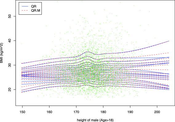
Figure 8: Regression spline estimates of conditional BMI quantiles in steps of $0.05$, from $0.1$ to $0.9$ for the NHANES data. Natural spline bases and six knots are used in each fitted curve.

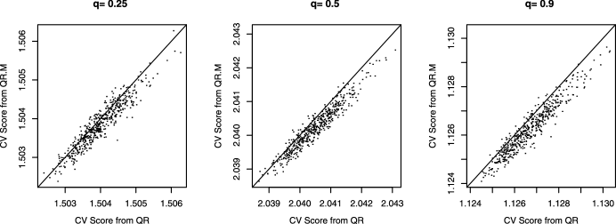
Figure 9: Scatterplots of 10-fold CV scores from standard quantile regression (QR) and modified quantile regression (QR.M) at $0.25$th, $0.5$th and $0.9$th quantiles. Regression splines with natural spline bases and six knots are fitted to the NHANES data. Each of 500 points represents a pair of CV scores as in (12).

The predictive performances of the standard and modified quantile regressions are compared in Figure 9. To compare the methods, $10$-fold cross-validation was repeated $500$ times for different splits of the data. Each time, a cross-validation score was computed as

$$\mathrm{CV}=\frac{1}{n}\sum_{i=1}^{n}\rho_{q}(y_{i}-\hat{y_{i}}),$$ (12)

where $y_{i}$ is the observed BMI for an individual in the hold-out sample, $\hat{y}_{i}$ is the fitted value under QR or QR.M, and the sum runs over the hold-out sample. The figure contains plots of the $500$ $\mathrm{CV}$ scores. The great majority of $\mathrm{CV}$ scores are to the lower right side of the 45 degree line, indicating that the modified quantile regression outperforms the standard method—even when the QR empirical risk function is used to evaluate performance. Mean and 1000 times standard deviation of the $\mathrm{CV}$ scores for the methods are summarized in Table 3.

The pattern shown in these panels is consistent across other quantiles (not shown here). The pattern becomes a bit stronger when the QR.M empirical risk function is used to evaluate performance.

Quantile regression has the property that $100\cdot q$% of the responses fall at or below the fitted $q$th quantile surface. This does not have to hold for the modified quantile regression fit. However, as the cross-validation shows, QR.M does provide a better quantile regression surface than QR.

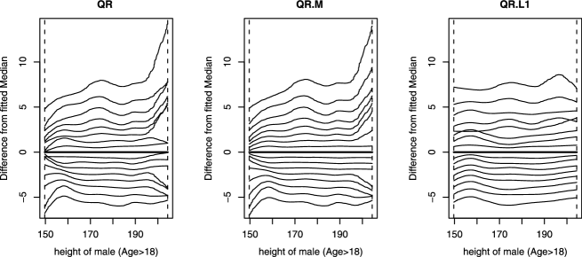
Figure 10: Differences between fitted median line and the other fitted quantiles for standard quantile regression (QR), modified quantile regression (QR.M), and $\ell_{1}$ penalized quantile regression (QR.L1) for the NHANES data. The dashed lines are the minimum and maximum of the observed heights.

Modified quantile regression has an additional advantage which is apparent for small and large heights. The standard quantile regression fits show several crossings of estimated quantiles, while crossing behavior is reduced considerably with modified quantile regression. Crossed quantiles correspond toa claim that a lower quantile lies above a higher quantile, contradicting the laws of probability. Figure 10 shows this behavior. Fixes for this behavior have been proposed (e.g., (He, 1997)), but we consider it desirable to lessen crossing without any explicit fix. The reduction in crossing holds up across other data sets that we have examined and with regression models that differ in their details.

Table 3: Mean and (1000 times standard deviation) of CV scores at selected quantiles based on 500 replicates from NHANES data

Method	$\bolds{q=0.25}$	$\bolds{q=0.5}$	$\bolds{q=0.9}$
QR	1.5040 (0.6105)	2.0405 (0.7272)	1.1267 (1.0714)
QR.M	1.5039 (0.5855)	2.0402 (0.6576)	1.1263 (1.0030)
QR.L1	1.5039 (0.8963)	2.0393 (0.5140)	1.1289 (0.8569)

In addition, we compare both methods with $\ell_{1}$ parameter-penalized quantile regression (QR.L1),where the estimator $\hat{\beta}$ is defined as the minimizer of

$$\sum_{i=1}^{n}\rho_{q}(y_{i}-x_{i}^{\top}\beta)+\lambda_{\beta}\sum_{j=1}^{p}|\beta_{j}|.$$

The rq.fit.lasso function in the quantreg R package was used for QR.L1. Keeping the same split of data into 90% of training and 10% of testing for each replicate, we have chosen $\lambda_{\beta}$ among 100 candidate values by 9-fold cross-validation. The results are in Table 3.

The effect of parameter penalization differs from modification of the loss function. Figure 10 illustrates the difference. The quantiles estimated under QR.L1 (with $\lambda_{\beta}$ chosen by 10-fold cross-validation) show less variation across $x$ relative to the fitted median line, due to the shrinkage of each $\beta_{j}$ toward 0. This effect is more visible for large quantiles. Such nondifferential penalty can degrade performance, unless the parameters are of comparable size. This adverse effect is numerically evidenced in the large $\mathrm{CV}$ score of QR.L1 for $q=0.9$ in Table 3. For $q=0.25$ and $0.5$, QR.L1 yields similar results to the other two methods in terms of the $\mathrm{CV}$ scores.

6.2 Analysis of Language Data

Balota et al. (2004) conducted an extensive lexical decision experiment in which subjects were asked to identify whether a string of letters was an English word or a nonword. The words were monosyllabic, and the nonwords were constructed to closely resemble words on a number of linguistic dimensions. Two groups were studied—college students and older adults. The data consist of response times by word, averaged over the thirty subjects in each group. For each word, a number of covariates was recorded. Goals of the experiment include determining which features of a word (i.e., covariates) affect response time, and whether the active features affect response time in the same fashion for college students and older adults. The authors make a case for the need to conduct and analyze studies with regression techniques in mind, rather than simpler ANOVA techniques.

Baayen (2007) conducted an extensive analysis of a slightly modified data set which is available in his languageR package. In his analysis, he creates and selects variables to include in a regression model, addresses issues of nonlinearity, collinearity and interaction, and removes selected cases as being influential and/or outlying. He trims a total of $87$ of the $4568$ cases. The resulting model, based on “typical” words, is used to address issues of linguistic importance. It includes seventeen basic covariates which enter the model as linear terms, a nonlinear term for the written frequency of a word (fit as a restricted cubic spline with five knots), and an interaction term between the age group and the (nonlinear) written frequency of the word.

We consider two sets of potential covariates for the model. The small set consists of Baayen’s $17$ basic covariates and three additional covariates representing a squared term for written frequency and the interaction between age group and the linear and squared terms for written frequency. Age group has been coded as $\pm 1$ for the interactions. The large set augments these covariates with nine additional covariates that were not included in Baayen’s final model. Baayen excluded some of these covariates for a lack of significance, others because of collinearity.

To investigate the performance of the LASSO and robust LASSO, a simulation study was conducted on the $4568$ cases in the data set. For a single replicate in the simulation, the data were partitioned into a training data set and a test data set. The various methods were fit to the training data, with evaluation conducted on the test data. The criteria for evaluation were sum of squared differences between the fitted and observed responses, either over all cases in the test data or over the test data with the cases identified by Baayen as outliers removed. We refer to these criteria as predictive mean squared error ($\mathrm{PMSE}$).

The simulation investigated several factors, including the amount of training data (10% of the full data, 20%, 30%, etc.), the regularization parameter $\lambda_{\gamma}=k\hat{\sigma}$, and the method used to select the model. Three methods were used to select the model (i.e., the fraction of the distance along the solution path): minimum $C_{p}$, generalized cross-validation, and 10-fold cross-validation on the training data.

The results of a $300$ replicate simulation show a convincing benefit to use of the robust LASSO. The benefit of the robust LASSO is most apparent when $k$ is in the “sweet spot” ranging from $1.4$ or so to well above $2.0$. As expected, for very small $k$ (near 1), the robust LASSO may not perform as well as the LASSO. The reduction in $\mathrm{PMSE}$ for moderate values of $k$, both absolute and percent, is slightly larger when the evaluation is conducted after outliers (as identified by Baayen—not by the fitted model) have been dropped from the test data set. The benefit is largest for small training data sets and decreases as the size of the training data set increases. For large training data sets (e.g., 90% of the data), little test data remains for calculation of $\mathrm{PMSE}$ and the evaluation is less stable. These patterns were apparent over all three methods of model selection. Figure 11 shows the results for a training sample size of $1827$ cases (40% of the data), with model selected by cross-validation, for a variety of values of $k$. The $\mathrm{PMSE}$ for the robust LASSO dips below the mean $\mathrm{PMSE}$ for the LASSO for a wide range of $k$. The figure also presents 95% confidence intervals, based on the $300$ replicates in the simulation, for the difference between mean $\mathrm{PMSE}$ under the robust LASSO and the LASSO. The intervals are indicated by the vertical lines, and statistical significance is indicated where the lines do not overlap the mean $\mathrm{PMSE}$ under the LASSO. The narrowing of the intervals is a consequence of the greater similarity of LASSO and robust LASSO fits as the bending constant increases. The patterns just described hold for both the small set of covariates and the large set of covariates.

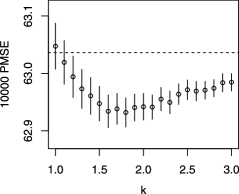
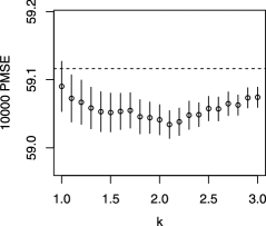
(a)	(b)

Figure 11: Predictive mean squared error (PMSE) for the test data in the simulation study, after removal of cases identified by Baayen as outliers. The horizontal line is the mean PMSE for the LASSO while the points represent the mean of PMSEs for the robust LASSO. The vertical lines have the width of approximate 95% confidence intervals for the difference in mean PMSE under the LASSO and robust LASSO. Panel (a) presents results for the small set of covariates and panel (b) presents results for the large set of covariates.

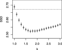
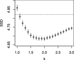
(a)	(b)

Figure 12: Sum of squared deviations (SSD) from Baayen’s fits in the simulation study. The horizontal line is the mean SSD for the LASSO while the points represent the mean of SSDs for the robust LASSO. The vertical lines have the width of approximate 95% confidence intervals for the difference in mean SSD under the LASSO and robust LASSO. Panel (a) presents results for the small set of covariates and panel (b) presents results for the large set of covariates.

In addition to using the test data as a target, we studied how well the two methods could reproduce Baayen’s expert fit. This makes a good target for inference, as there is evidence that humans can produce a better fit than automated methods ((Yu, MacEachern and Peruggia, 2011)). Taking a fitted surface as a target allows us to remove the noise inherent in data-based out-of-sample evaluations.The results from a $5000$ replicate simulation study with a training sample size of $400$ appear in Figure 12. The criterion is sum of squared deviations ($\mathrm{SSD}$) between the (robust) LASSO fit and Baayen’s fit, with the sum taken over only those covariate values contained in the test data set. The results presented here are for models selected with the minimum $C_{p}$ criterion. The robust LASSO outperforms the LASSO over a wide range of values for $k$ for both the small and large sets of covariates.

Figures 11 and 12 reveal an interesting difference across targets in the behavior of the small and large sets of covariates. When the target is an expert fit, as in the second study, adding covariates not present in the expert’s model to the pool of potential covariates allows the LASSO and robust LASSO to produce a near-equivalent fit to the data, but with different coefficients for the regressors. An examination of the variables present in the fitted models and their coefficients uncovers patterns. As an example, the two covariates “WrittenFrequency” and “Familiarity” appear in nearly all of the models for both the LASSO and the robust LASSO, while Baayen includes only “WrittenFrequency” in his model, and these covariate(s) have negative coefficients. Subjects are able to decide that a familiar word is a word more quickly (and more accurately) than an unfamiliar word. Although there seems to be no debate on whether this conceptual effect of similarity exists, there are a variety of viewpoints on how to best capture the effect. Regularization methods allow one to include a suite of covariates to address a single conceptual effect, and this produces a difference between the LASSO and robust LASSO fits on one hand and a least-squares, variable-selection style fit on the other hand. The end result is that the regularized fits with the large set of covariates show greater departures from Baayen’s fit than do regularized fits with the small set of covariates. In contrast, under the data-based target of the first study, the large set of covariates results in a smaller $\mathrm{PMSE}$.

7 Discussion

In the preceding sections, we have laid out an approach to modifying modeling procedures. The approach is based on the creation of case-specific covariates which are then regularized. With appropriate choices of penalty terms, the addition of these covariates allows us to robustify those procedures which lack robustness and also allows us to improve the efficiency of procedures which are very robust, but not particularly efficient. The method is fully compatible with regularized estimation methods. In this case, the case-specific covariates are merely included as part of the regularization. The techniques are easy to implement, as they often require little modification of existing software. In some cases, there is no need for modification of software, as one merely feeds a modified data set into existing routines.

The motivation behind this work is a desire to move relatively automated modeling procedures in the direction of traditional data analysis (e.g., Weisberg, 2004). An important component of this type of analysis is the ability to take different looks at a data set. These different looks may suggest creation of new variates and differential handling of individual cases or groups of cases. Robust methods allow us to take such a look, even when data sets are large. Coupling robust regression techniques with the ability to examine an entire solution path provides a sharper view of the impact of unusual cases on the analysis. A second motivation for the work is the desire to improve robust, relatively nonparametric methods. This is accomplished by introducing case-specific parameters in a controlled fashion whereby the finite sample performance of estimators is improved.

The perspective provided by this work suggests several directions for future research. Adaptive penalties, whether used for robustness or efficiency, can be designed to satisfy specified invariances. The asymmetric $\ell_{2}$ penalty for modified quantile regression was designed to satisfy a specified invariance. For a locally constant residual density, it keeps the $0$ of the $\psi_{q}^{\gamma}$ function invariant as the width of the interval of adjustment varies. Specific, alternative forms of invariance for quantile regression are suggested by consideration of parametric driving forms for the residual distribution. A motivating parametric model, coupled with invariance of the $0$ of the $\psi_{q}^{\gamma}$ function to the size of the penalty term $\lambda_{\gamma}$, yields a path of penalties. Increasing the size of the covariate-specific penalty at an appropriate rate leads to asymptotic equivalence with the quantile regression estimator. This allows one to fit the model nonparametrically while tapping into an approximate parametric form to enhance finite sample performance. Similarly, when case-specific penalties are applied to a model such as the generalized linear model, the asymmetry of the likelihood, coupled with invariance, suggests an asymmetric form for the $\ell_{1}$ penalty used to enhance robustness of inference.

Following development of the technique for quantile regression, one can apply the adaptive loss paradigm for model assessment and selection. For example, in cross-validation, a summary of a model’s fit is computed as an out-of-sample estimate of empirical risk and the evaluation is used for choosing the model (parameter value) with the smallest estimated risk. For model averaging, estimated risks are converted into weights which are then attached to model-specific predictions that are then combined to yield an overall prediction. The use of modified loss functions for estimation of risks is expected to improve stability and efficiency in model evaluation and selection.

Appendix

Proof of Theorem 2. Let $u_{i}:=y_{i}-x_{i}^{\top}\beta(q)$ and consider the objective function

$$\quad Z_{n}^{\gamma}(\delta):=\sum^{n}_{i=1}\bigl{\{}\rho_{q}^{\gamma}\bigl{(}u_{i}-x_{i}^{\top}\delta/\sqrt{n}\bigr{)}-\rho_{q}(u_{i})\bigr{\}}.$$ (13)

Note that $Z_{n}^{\gamma}(\delta)$ is minimized at $\hat{\delta}_{n}:=\sqrt{n}(\hat{\beta}^{\gamma}_{n}-\beta(q))$, and the limiting distribution of $\hat{\delta}_{n}$ is determined by the limiting behavior of $Z_{n}^{\gamma}(\delta)$. To study the limit of $Z_{n}^{\gamma}(\delta)$, decompose $Z_{n}^{\gamma}(\delta)$ as

$$Z_{n}^{\gamma}(\delta) = \sum^{n}_{i=1}\bigl{\{}\rho_{q}^{\gamma}\bigl{(}u_{i}-x_{i}^{\top}\delta/\sqrt{n}\bigr{)}-\rho_{q}\bigl{(}u_{i}-x_{i}^{\top}\delta/\sqrt{n}\bigr{)}\bigr{\}}$$

$${}+\sum^{n}_{i=1}\bigl{\{}\rho_{q}\bigl{(}u_{i}-x_{i}^{\top}\delta/\sqrt{n}\bigr{)}-\rho_{q}(u_{i})\bigr{\}}$$

$$= \sum^{n}_{i=1}\bigl{\{}\rho_{q}^{\gamma}\bigl{(}u_{i}-x_{i}^{\top}\delta/\sqrt{n}\bigr{)}-\rho_{q}\bigl{(}u_{i}-x_{i}^{\top}\delta/\sqrt{n}\bigr{)}\bigr{\}}$$

$${}+Z_{n}(\delta),$$

where $Z_{n}(\delta):=\sum^{n}_{i=1}\{\rho_{q}(u_{i}-x_{i}^{\top}\delta/\sqrt{n})-\rho_{q}(u_{i})\}$. By showing that the first sum converges to zero in probability up to a sequence of constants that do not depend on $\delta$, we will establish the asymptotic equivalence of $\hat{\beta}^{\gamma}_{n}$ to $\hat{\beta}_{n}$.

Given $\lambda_{\gamma}=cn^{\alpha}$, first observe that

$$E\bigl{\{}\rho_{q}^{\gamma}\bigl{(}u_{i}-x_{i}^{\top}\delta/\sqrt{n}\bigr{)}-\rho_{q}\bigl{(}u_{i}-x_{i}^{\top}\delta/\sqrt{n}\bigr{)}\bigr{\}}$$

$$\qquad{}+q(1-q)/2\lambda_{\gamma}$$

$$\quad=\int^{{(1-q)}/{\lambda_{\gamma}}+x_{i}^{\top}\delta/\sqrt{n}}_{x_{i}^{\top}\delta/\sqrt{n}}\biggl{(}\frac{\lambda_{\gamma}}{2}\frac{q}{1-q}\biggl{(}u-\frac{x_{i}^{\top}\delta}{\sqrt{n}}\biggr{)}^{2}$$

$$\hskip 82.0pt\qquad{}-q\biggl{(}u-\frac{x_{i}^{\top}\delta}{\sqrt{n}}\biggr{)}+\frac{q(1-q)}{2\lambda_{\gamma}}\biggr{)}$$

$$\hskip 101.0pt\cdot f_{i}(\xi_{i}+u)\,du$$

$$\qquad{}+\int^{x_{i}^{\top}\delta/\sqrt{n}}_{-q/{\lambda_{\gamma}}+x_{i}^{\top}\delta/\sqrt{n}}\biggl{(}\frac{\lambda_{\gamma}}{2}\frac{1-q}{q}\biggl{(}u-\frac{x_{i}^{\top}\delta}{\sqrt{n}}\biggr{)}^{2}$$

$$\hskip 79.0pt\qquad{}-(q-1)\biggl{(}u-\frac{x_{i}^{\top}\delta}{\sqrt{n}}\biggr{)}$$

$$\hskip 128.0pt\qquad{}+\frac{q(1-q)}{2\lambda_{\gamma}}\biggr{)}$$

$$\hskip 96.0pt{}\cdot f_{i}(\xi_{i}+u)\,du$$

$$\quad=\int^{{(1-q)}/{\lambda_{\gamma}}+x_{i}^{\top}\delta/\sqrt{n}}_{x_{i}^{\top}\delta/\sqrt{n}}\frac{\lambda_{\gamma}}{2}\frac{q}{1-q}$$

$$\hskip 79.0pt\qquad{}\cdot\biggl{(}u-\frac{x_{i}^{\top}\delta}{\sqrt{n}}-\frac{1-q}{\lambda_{\gamma}}\biggr{)}^{2}$$

$$\hskip 79.0pt\qquad{}\cdot f_{i}(\xi_{i}+u)\,du$$

$$\qquad{}+\int^{x_{i}^{\top}\delta/\sqrt{n}}_{-q/{\lambda_{\gamma}}+x_{i}^{\top}\delta/\sqrt{n}}\frac{\lambda_{\gamma}}{2}\frac{1-q}{q}\biggl{(}u-\frac{x_{i}^{\top}\delta}{\sqrt{n}}+\frac{q}{\lambda_{\gamma}}\biggr{)}^{2}$$

$$\hskip 79.0pt\qquad{}\cdot f_{i}(\xi_{i}+u)\,du.$$

Using a first-order Taylor expansion of $f_{i}$ at $\xi_{i}$ from the condition (C-2) and the expression above, we have

$$E\sum^{n}_{i=1}\bigl{\{}\rho_{q}^{\gamma}\bigl{(}u_{i}-x_{i}^{\top}\delta/\sqrt{n}\bigr{)}-\rho_{q}\bigl{(}u_{i}-x_{i}^{\top}\delta/\sqrt{n}\bigr{)}\bigr{\}}$$

$$\qquad{}+nq(1-q)/2\lambda_{\gamma}$$

$$\quad=\frac{q(1-q)}{6c^{2}n^{2\alpha}}\sum^{n}_{i=1}f_{i}(\xi_{i})+\frac{q(1-q)}{6c^{2}n^{2\alpha}}\sum^{n}_{i=1}\frac{f^{\prime}_{i}(\xi_{i})x_{i}^{\top}\delta}{\sqrt{n}}$$

$$\qquad{}+o(n^{-2\alpha+1/2}).$$

Note that $\sum^{n}_{i=1}f^{\prime}_{i}(\xi_{i})x_{i}^{\top}\delta/\sqrt{n}=O(\sqrt{n})$ as $f^{\prime}_{i}(\xi_{i})$, $i=1,\ldots,n$, are uniformly bounded from the condition (C-2), and $|x_{i}^{\top}\delta|\leq\|x_{i}\|_{2}\|\delta\|_{2}\leq(\|x_{i}\|_{2}^{2}+\|\delta\|_{2}^{2})/2$ while $\sum^{n}_{i=1}\|x_{i}\|_{2}^{2}=O(n)$ from the condition (C-3). Taking $C_{n}:=-{q(1-q)}/{(2cn^{\alpha-1})}+{q(1-q)}/\break{(6c^{2}n^{2\alpha})}\sum^{n}_{i=1}f_{i}(\xi_{i})$, we have that

$$E\sum^{n}_{i=1}\bigl{\{}\rho_{q}^{\gamma}\bigl{(}u_{i}-x_{i}^{\top}\delta/\sqrt{n}\bigr{)}-\rho_{q}\bigl{(}u_{i}-x_{i}^{\top}\delta/\sqrt{n}\bigr{)}\bigr{\}}-C_{n}$$

$$\quad{}\rightarrow 0\quad\mbox{if }\alpha>1/4.$$

Similarly, it can be shown that

$$\operatorname{Var}\sum^{n}_{i=1}\bigl{\{}\rho_{q}^{\gamma}\bigl{(}u_{i}-x_{i}^{\top}\delta/\sqrt{n}\bigr{)}-\rho_{q}\bigl{(}u_{i}-x_{i}^{\top}\delta/\sqrt{n}\bigr{)}\bigr{\}}$$

$$\quad=\sum^{n}_{i=1}\frac{q^{2}(1-q)^{2}f_{i}(\xi_{i})}{20c^{3}n^{3\alpha}}+o(n^{-3\alpha+1})$$

$$\qquad\rightarrow 0\quad\mbox{if }\alpha>1/3.$$

Thus, if $\alpha$ $>1/3$,

$$\sum^{n}_{i=1}\rho_{q}^{\gamma}\bigl{(}u_{i}-x_{i}^{\top}\delta/\sqrt{n}\bigr{)}-\rho_{q}\bigl{(}u_{i}-x_{i}^{\top}\delta/\sqrt{n}\bigr{)}-C_{n}$$

$$\quad\rightarrow 0\quad\mbox{in probability}.$$

This implies that the limiting behavior of $Z_{n}^{\gamma}(\delta)$ is the same as that of $Z_{n}(\delta)$. From the proof of Theorem 4.1 in Koenker (2005), $Z_{n}(\delta)\stackrel{{\scriptstyle d}}{{\rightarrow}}-\delta^{\top}W+\frac{1}{2}\delta^{\top}D_{1}\delta$, where $W$ $\sim N(0,q(1-q)D_{0})$. By the convexity argument in Koenker (2005) (see also (Pollard, 1991); (Hjort and Pollard, 1993); (Knight, 1998)), $\hat{\delta}_{n}$, the minimizer of $Z_{n}^{\gamma}(\delta)$, converges to $\hat{\delta}_{0}:=D_{1}^{-1}W$, the unique minimizer of $-\delta^{\top}W+\frac{1}{2}\delta^{\top}D_{1}\delta$ in distribution. This completes the proof.

References

- Baayen (2007) {bbook}[author] \bauthor\bsnmBaayen, \bfnmR. H.\binitsR. H. (\byear2007). \btitleAnalyzing Linguistic Data: A Practical Introduction to Statistics. \bpublisherCambridge Univ. Press, \baddressCambridge, England. \bptokimsref \endbibitem
- Balota et al. (2004) {barticle}[author] \bauthor\bsnmBalota, \bfnmD. A.\binitsD. A., \bauthor\bsnmCortese, \bfnmM. J.\binitsM. J., \bauthor\bsnmSergent-Marshall, \bfnmS. D.\binitsS. D., \bauthor\bsnmSpieler, \bfnmD. H.\binitsD. H. and \bauthor\bsnmYap, \bfnmM. J.\binitsM. J. (\byear2004). \btitleVisual word recognition of single-syllable words. \bjournalJournal of Experimental Psychology \bvolume133 \bpages283–316. \bptokimsref \endbibitem
- Bartlett, Jordan and McAuliffe (2006) {barticle}[mr] \bauthor\bsnmBartlett, \bfnmPeter L.\binitsP. L., \bauthor\bsnmJordan, \bfnmMichael I.\binitsM. I. and \bauthor\bsnmMcAuliffe, \bfnmJon D.\binitsJ. D. (\byear2006). \btitleConvexity, classification, and risk bounds. \bjournalJ. Amer. Statist. Assoc. \bvolume101 \bpages138–156. \biddoi=10.1198/016214505000000907, issn=0162-1459, mr=2268032 \bptokimsref \endbibitem
- Bi et al. (2003) {barticle}[author] \bauthor\bsnmBi, \bfnmJ.\binitsJ., \bauthor\bsnmBennett, \bfnmK.\binitsK., \bauthor\bsnmEmbrechts, \bfnmM.\binitsM., \bauthor\bsnmBreneman, \bfnmC.\binitsC. and \bauthor\bsnmSong, \bfnmM.\binitsM. (\byear2003). \btitleDimensionality reduction via sparse support vector machines. \bjournalJ. Mach. Learn. Res. \bvolume3 \bpages1229–1243. \bptokimsref \endbibitem
- Efron (1991) {barticle}[mr] \bauthor\bsnmEfron, \bfnmB.\binitsB. (\byear1991). \btitleRegression percentiles using asymmetric squared error loss. \bjournalStatist. Sinica \bvolume1 \bpages93–125. \bidissn=1017-0405, mr=1101317 \bptokimsref \endbibitem
- Efron et al. (2004a) {barticle}[mr] \bauthor\bsnmEfron, \bfnmBradley\binitsB., \bauthor\bsnmHastie, \bfnmTrevor\binitsT., \bauthor\bsnmJohnstone, \bfnmIain\binitsI. and \bauthor\bsnmTibshirani, \bfnmRobert\binitsR. (\byear2004a). \btitleLeast angle regression (with discussion, and a rejoinder by the authors). \bjournalAnn. Statist. \bvolume32 \bpages407–499. \biddoi=10.1214/009053604000000067, issn=0090-5364, mr=2060166 \bptnotecheck related\bptokimsref \endbibitem
- Fischler and Bolles (1981) {barticle}[mr] \bauthor\bsnmFischler, \bfnmMartin A.\binitsM. A. and \bauthor\bsnmBolles, \bfnmRobert C.\binitsR. C. (\byear1981). \btitleRandom sample consensus: A paradigm for model fitting with applications to image analysis and automated cartography. \bjournalComm. ACM \bvolume24 \bpages381–395. \biddoi=10.1145/358669.358692, issn=0001-0782, mr=0618158 \bptokimsref \endbibitem
- Freund and Schapire (1997) {barticle}[mr] \bauthor\bsnmFreund, \bfnmYoav\binitsY. and \bauthor\bsnmSchapire, \bfnmRobert E.\binitsR. E. (\byear1997). \btitleA decision-theoretic generalization of on-line learning and an application to boosting. \bjournalJ. Comput. System Sci. \bvolume55 \bpages119–139. \biddoi=10.1006/jcss.1997.1504, issn=0022-0000, mr=1473055 \bptokimsref \endbibitem
- Hastie and Tibshirani (1990) {bbook}[mr] \bauthor\bsnmHastie, \bfnmT. J.\binitsT. J. and \bauthor\bsnmTibshirani, \bfnmR. J.\binitsR. J. (\byear1990). \btitleGeneralized Additive Models. \bseriesMonographs on Statistics and Applied Probability \bvolume43. \bpublisherChapman & Hall, \baddressLondon. \bidmr=1082147 \bptokimsref \endbibitem
- Hastie et al. (2004) {barticle}[mr] \bauthor\bsnmHastie, \bfnmTrevor\binitsT., \bauthor\bsnmRosset, \bfnmSaharon\binitsS., \bauthor\bsnmTibshirani, \bfnmRobert\binitsR. and \bauthor\bsnmZhu, \bfnmJi\binitsJ. (\byear2004). \btitleThe entire regularization path for the support vector machine. \bjournalJ. Mach. Learn. Res. \bvolume5 \bpages1391–1415. \bidissn=1532-4435, mr=2248021 \bptnotecheck year\bptokimsref \endbibitem
- He (1997) {barticle}[author] \bauthor\bsnmHe, \bfnmXuming\binitsX. (\byear1997). \btitleQuantile curves without crossing. \bjournalAmer. Statist. \bvolume51 \bpages186–192. \bptokimsref \endbibitem
- Hjort and Pollard (1993) {bmisc}[author] \bauthor\bsnmHjort, \bfnmNils Lid\binitsN. L. and \bauthor\bsnmPollard, \bfnmDavid\binitsD. (\byear1993). \bhowpublishedAsymptotics for minimisers of convex processes. Technical report, Dept. Statistics, Yale Univ. \bptokimsref \endbibitem
- Hoerl and Kennard (1970) {barticle}[author] \bauthor\bsnmHoerl, \bfnmA. E.\binitsA. E. and \bauthor\bsnmKennard, \bfnmR. W.\binitsR. W. (\byear1970). \btitleRidge regression: Biased estimation for nonorthogonal problems. \bjournalTechnometrics \bvolume12 \bpages55–67. \bptokimsref \endbibitem
- Huber (1981) {bbook}[mr] \bauthor\bsnmHuber, \bfnmPeter J.\binitsP. J. (\byear1981). \btitleRobust Statistics. \bpublisherWiley, \baddressNew York. \bidmr=0606374 \bptokimsref \endbibitem
- Jung, MacEachern and Lee (2010) {bmisc}[author] \bauthor\bsnmJung, \bfnmYoonsuh\binitsY., \bauthor\bsnmMacEachern, \bfnmSteven N.\binitsS. N. and \bauthor\bsnmLee, \bfnmYoonkyung\binitsY. (\byear2010). \bhowpublishedWindow width selection for adjusted quantile regression. Technical Report 835, Dept. Statistics, Ohio State Univ. \bptokimsref \endbibitem
- Knight (1998) {barticle}[mr] \bauthor\bsnmKnight, \bfnmKeith\binitsK. (\byear1998). \btitleLimiting distributions for regression estimators under general conditions. \bjournalAnn. Statist. \bvolume26 \bpages755–770. \biddoi=10.1214/aos/1028144858, issn=0090-5364, mr=1626024 \bptokimsref \endbibitem
- Koenker (2005) {bbook}[mr] \bauthor\bsnmKoenker, \bfnmRoger\binitsR. (\byear2005). \btitleQuantile Regression. \bseriesEconometric Society Monographs \bvolume38. \bpublisherCambridge Univ. Press, \baddressCambridge. \biddoi=10.1017/CBO9780511754098, mr=2268657 \bptokimsref \endbibitem
- Koenker and Bassett (1978) {barticle}[mr] \bauthor\bsnmKoenker, \bfnmRoger\binitsR. and \bauthor\bsnmBassett, \bfnmGilbert\binitsG., \bsuffixJr. (\byear1978). \btitleRegression quantiles. \bjournalEconometrica \bvolume46 \bpages33–50. \bidissn=0012-9682, mr=0474644 \bptokimsref \endbibitem
- Koenker and Hallock (2001) {barticle}[author] \bauthor\bsnmKoenker, \bfnmR.\binitsR. and \bauthor\bsnmHallock, \bfnmK.\binitsK. (\byear2001). \btitleQuantile regression. \bjournalJournal of Economic Perspectives \bvolume15 \bpages143–156. \bptokimsref \endbibitem
- Lee, MacEachern and Jung (2007) {bmisc}[author] \bauthor\bsnmLee, \bfnmYoonkyung\binitsY., \bauthor\bsnmMacEachern, \bfnmSteven N.\binitsS. N. and \bauthor\bsnmJung, \bfnmYoonsuh\binitsY. (\byear2007). \bhowpublishedRegularization of case-specific parameters for robustness and efficiency. Technical Report 799, Dept. Statistics, Ohio State Univ. \bptokimsref \endbibitem
- Lee and Mangasarian (2001) {barticle}[mr] \bauthor\bsnmLee, \bfnmYuh-Jye\binitsY.-J. and \bauthor\bsnmMangasarian, \bfnmO. L.\binitsO. L. (\byear2001). \btitleSSVM: A smooth support vector machine for classification. \bjournalComput. Optim. Appl. \bvolume20 \bpages5–22. \biddoi=10.1023/A:1011215321374, issn=0926-6003, mr=1849977 \bptokimsref \endbibitem
- Lee and Wang (2011) {bmisc}[author] \bauthor\bsnmLee, \bfnmYoonkyung\binitsY. and \bauthor\bsnmWang, \bfnmRui\binitsR. (\byear2011). \bhowpublishedDoes modeling lead to more accurate classification?: A study of relative efficiency. Unpublished manuscript. \bptokimsref \endbibitem
- McCullagh and Nelder (1989) {bbook}[author] \bauthor\bsnmMcCullagh, \bfnmP.\binitsP. and \bauthor\bsnmNelder, \bfnmJ.\binitsJ. (\byear1989). \btitleGeneralized Linear Models, \bedition2nd ed. \bpublisherChapman & Hall/CRC, \baddressBoca Raton, FL. \bptokimsref \endbibitem
- Newey and Powell (1987) {barticle}[mr] \bauthor\bsnmNewey, \bfnmWhitney K.\binitsW. K. and \bauthor\bsnmPowell, \bfnmJames L.\binitsJ. L. (\byear1987). \btitleAsymmetric least squares estimation and testing. \bjournalEconometrica \bvolume55 \bpages819–847. \biddoi=10.2307/1911031, issn=0012-9682, mr=0906565 \bptokimsref \endbibitem
- Nychka et al. (1995) {barticle}[author] \bauthor\bsnmNychka, \bfnmD.\binitsD., \bauthor\bsnmGray, \bfnmG.\binitsG., \bauthor\bsnmHaaland, \bfnmP.\binitsP., \bauthor\bsnmMartin, \bfnmD.\binitsD. and \bauthor\bsnmO’Connell, \bfnmM.\binitsM. (\byear1995). \btitleA nonparametric regression approach to syringe grading for quality improvement. \bjournalJ. Amer. Statist. Assoc. \bvolume90 \bpages1171–1178. \bptokimsref \endbibitem
- Pollard (1991) {barticle}[mr] \bauthor\bsnmPollard, \bfnmDavid\binitsD. (\byear1991). \btitleAsymptotics for least absolute deviation regression estimators. \bjournalEconometric Theory \bvolume7 \bpages186–199. \biddoi=10.1017/S0266466600004394, issn=0266-4666, mr=1128411 \bptokimsref \endbibitem
- Portnoy and Koenker (1997) {barticle}[mr] \bauthor\bsnmPortnoy, \bfnmStephen\binitsS. and \bauthor\bsnmKoenker, \bfnmRoger\binitsR. (\byear1997). \btitleThe Gaussian hare and the Laplacian tortoise: Computability of squared-error versus absolute-error estimators. \bjournalStatist. Sci. \bvolume12 \bpages279–300. \biddoi=10.1214/ss/1030037960, issn=0883-4237, mr=1619189 \bptnotecheck related\bptokimsref \endbibitem
- Pregibon (1982) {barticle}[author] \bauthor\bsnmPregibon, \bfnmDaryl\binitsD. (\byear1982). \btitleResistant fits for some commonly used logistic models with medical applications. \bjournalBiometrics \bvolume38 \bpages485–498. \bptokimsref \endbibitem
- Rockafellar (1997) {bbook}[mr] \bauthor\bsnmRockafellar, \bfnmR. Tyrrell\binitsR. T. (\byear1997). \btitleConvex Analysis. \bpublisherPrinceton Univ. Press, \baddressPrinceton, NJ. \bidmr=1451876 \bptokimsref \endbibitem
- Rosset and Zhu (2004) {barticle}[author] \bauthor\bsnmRosset, \bfnmSaharon\binitsS. and \bauthor\bsnmZhu, \bfnmJi\binitsJ. (\byear2004). \btitleDiscussion of “Least angle regression,” by B. Efron, T. Hastie, I. Johnstone and R. Tibshirani. \bjournalAnn. Statist. \bvolume32 \bpages469–475. \bptokimsref \endbibitem
- Rosset and Zhu (2007) {barticle}[mr] \bauthor\bsnmRosset, \bfnmSaharon\binitsS. and \bauthor\bsnmZhu, \bfnmJi\binitsJ. (\byear2007). \btitlePiecewise linear regularized solution paths. \bjournalAnn. Statist. \bvolume35 \bpages1012–1030. \biddoi=10.1214/009053606000001370, issn=0090-5364, mr=2341696 \bptokimsref \endbibitem
- Shen et al. (2003) {barticle}[mr] \bauthor\bsnmShen, \bfnmXiaotong\binitsX., \bauthor\bsnmTseng, \bfnmGeorge C.\binitsG. C., \bauthor\bsnmZhang, \bfnmXuegong\binitsX. and \bauthor\bsnmWong, \bfnmWing Hung\binitsW. H. (\byear2003). \btitleOn -learning. \bjournalJ. Amer. Statist. Assoc. \bvolume98 \bpages724–734. \biddoi=10.1198/016214503000000639, issn=0162-1459, mr=2011686 \bptokimsref \endbibitem
- Tibshirani (1996) {barticle}[mr] \bauthor\bsnmTibshirani, \bfnmRobert\binitsR. (\byear1996). \btitleRegression shrinkage and selection via the lasso. \bjournalJ. Roy. Statist. Soc. Ser. B \bvolume58 \bpages267–288. \bidissn=0035-9246, mr=1379242 \bptokimsref \endbibitem
- Vapnik (1998) {bbook}[mr] \bauthor\bsnmVapnik, \bfnmVladimir N.\binitsV. N. (\byear1998). \btitleStatistical Learning Theory. \bpublisherWiley, \baddressNew York. \bidmr=1641250 \bptokimsref \endbibitem
- Wahba (1990) {bbook}[mr] \bauthor\bsnmWahba, \bfnmGrace\binitsG. (\byear1990). \btitleSpline Models for Observational Data. \bseriesCBMS-NSF Regional Conference Series in Applied Mathematics \bvolume59. \bpublisherSIAM, \baddressPhiladelphia, PA. \bidmr=1045442 \bptokimsref \endbibitem
- Weisberg (2004) {barticle}[author] \bauthor\bsnmWeisberg, \bfnmSanford\binitsS. (\byear2004). \btitleDiscussion of “Least angle regression,” by B. Efron, T. Hastie, I. Johnstone and R. Tibshirani. \bjournalAnn. Statist. \bvolume32 \bpages490–494. \bptokimsref \endbibitem
- Weisberg (2005) {bbook}[mr] \bauthor\bsnmWeisberg, \bfnmSanford\binitsS. (\byear2005). \btitleApplied Linear Regression, \bedition3rd ed. \bpublisherWiley-Interscience, \baddressHoboken, NJ. \biddoi=10.1002/0471704091, mr=2112740 \bptokimsref \endbibitem
- Wu and Liu (2007) {barticle}[mr] \bauthor\bsnmWu, \bfnmYichao\binitsY. and \bauthor\bsnmLiu, \bfnmYufeng\binitsY. (\byear2007). \btitleRobust truncated hinge loss support vector machines. \bjournalJ. Amer. Statist. Assoc. \bvolume102 \bpages974–983. \biddoi=10.1198/016214507000000617, issn=0162-1459, mr=2411659 \bptokimsref \endbibitem