Freezing of a two dimensional fluid into a crystalline phase : Density functional approach

Abstract

A free-energy functional for a crystal proposed by Singh and Singh (Europhys. Lett. 88, 16005 (2009)) and which contains both the symmetry conserved and symmetry broken parts of the direct pair correlation function has been used to investigate the crystallization of a two-dimensional fluid. The results found for fluids interacting via the inverse power potential $u(r)=\epsilon\left({\sigma}/{r}\right)^{n}$ for n= 3, 6 and 12 are in good agreement with experimental and simulation results. The contribution made by the symmetry broken part to the grand thermodynamic potential at the freezing point is found to increase with the softness of the potential. Our results explain why the Ramakrishnan-Yussouff (Phys. Rev. B 19, 2775 (1979)) free-energy functional gave good account of freezing transitions of hard-core potentials but failed for potentials that have soft core and/or attractive tail.

I Introduction

Freezing is a basic phenomenon, the most inevitable of all phase changes. When a liquid freezes into a crystalline solid its continuous symmetry of translation and rotation is broken into one of the Bravais lattices. A crystalline solid has a discrete set of vectors $\bf{R}_{i}$ such that any function of position such as one particle density $\rho(\bf{r})$ satisfies $\rho(\bf{r}+\bf{R}_{i})=\rho(\bf{r})$ for all $\bf{R}_{i}$ [1]. Because of localization of particles on lattice sites, a crystal is a system of extreme inhomogeneities where values of $\rho(\bf{r})$ show extreme differences between its values on the lattice sites and in the interstitial regions. The density functional formalism of classical statistical mechanics has been used to develop theories for liquid- solid transitions [2, 3]. This kind of approach was initiated in 1979 by Ramakrishnan and Yussouff [4].

The central quantity in this formulation is the excess reduced Helmholtz free energy due to interparticle interactions of both the crystal $A_{ex}[\rho]$ and the liquid $A_{ex}[\rho_{l}]$ [4,5]. For the crystal $A_{ex}[\rho]$ is a unique functional of $\rho{({\bf r})}$ whereas for the liquid $A_{ex}(\rho_{l})$ is simply a function of liquid density $\rho_{l}$. The density functional formalism is used to write an expression for $A_{ex}[\rho]$ in terms of one and two-particle distribution functions of the solid [2-5]. The direct pair correlation function (DPCF) that appears in this expression is a functional of $\rho({\bf r})$ [2]. When this functional dependence is ignored and the DPCF is replaced by that of the coexisting uniform liquid [4,5] or by that of an “ effective uniform fluid ” [6,7] the free energy functional becomes approximate and fails to provide an accurate description of freezing transitions for a large class of intermolecular potentials. Attempts to include a term involving the three - body direct correlation function of the coexisting liquid in the free energy functional failed to improve the situation [8, 9].

It has recently been emphasized [10-12] that at the freezing point a qualitatively new contribution to the correlations in distribution of particles emerges due to spontaneous symmetry breaking. This fact has been used to write the DPCF of a frozen phase as a sum of two qualitatively different contributions; one that preserves the continuous symmetry of uniform liquid and the other that breaks it and vanishes in the liquid. The double functional integration in density space of a relation that connects $A_{ex}[\rho]$ to the DPCF led to an exact expression for $A_{ex}[\rho]$. The freezing transitions in three-dimensions have been investigated using this new free energy functional. The results found for the isotropic-nematic transition [10], crystallization of power-law fluids [11] and the freezing of fluids of hard spheres into crystalline and glassy phases [12] are very encouraging.

In this paper we apply the free energy functional to investigate the liquid-solid transition in two-dimensions. It may, however, be noted that in contrast to three-dimensional solid, a two-dimensional solid melts in two-steps; the intermediate phase known as hexatic has a very narrow stability region in between liquid and crystal [13-15]. Since inclusion of the hexatic phase in the density functional formalism has not so for been possible, we neglect its presence and focus on the freezing of a fluid into the crystalline phase. Similar approach has been taken by others [16-21]. Here our motivation is to examine how well this new free energy functional (described briefly in the following section) compares with other free energy functionals in describing the crystallization of two-dimensional fluids.

The paper is organized as follow : In Sec. II we give a brief description of the free-energy functional for a symmetry broken phase that contains both the symmetry-conserving and symmetry-broken parts of the DPCF. In Sec. III we describe methods to calculate these correlation functions for a two-dimensional system. The theory is applied in Sec. IV to investigate the freezing of power-law fluids into a crystalline solid of hexagonal lattice. The paper ends with a brief summary and perspectives in Sec. V.

II Free Energy Functional

The reduced free energy functional $A[\rho]$ of an inhomogeneous system is functional of $\rho({\bf r})$ and is written as [2]

$$A[\rho]=A_{id}[\rho]+A_{ex}[\rho].\hskip 156.49014pt(2.1)$$

The ideal gas part $A_{id}$ is exactly known and is written in terms of $\rho({\bf r})$ as

$$A_{id}[\rho]=\int{d{\bf r}\rho({\bf r})[ln(\rho({\bf r})\Lambda)-1]},\hskip 113.81102pt(2.2)$$

where $\Lambda$ is a cube of the thermal wavelength associated with a molecule. The second functional derivative of the excess part $A_{ex}[\rho]$ with respect to $\rho({\bf r})$ defines the DPCF $c({\bf r}_{1},{\bf r}_{2})$ of the system [2],

$$\frac{\delta^{2}A_{ex}[\rho]}{\delta\rho({\bf r}_{1})\delta\rho({\bf r}_{2})}=-c({\bf r}_{1},{\bf r}_{2},[\rho]).\hskip 142.26378pt(2.3)$$

The function $c$ that appears in this equation is related to the total correlation function $h({\bf r}_{1},{\bf r}_{2})$ through the Ornstein -Zernike(OZ) equation,

$$h({\bf r}_{1},{\bf r}_{2})=c({\bf r}_{1},{\bf r}_{2})+\int d{\bf r}_{3}c({\bf r}_{1},{\bf r}_{3})\rho({\bf r}_{3})h({\bf r}_{2},{\bf r}_{3}).\hskip 56.9055pt(2.4)$$

Both functions h and c are functional of $\rho({\bf r})$

Since breaking of continuous symmetry of a uniform liquid at the freezing point gives rise to a qualitatively new contribution to correlations in the distribution of particles [10-12], the DPCF of the frozen phase is written as a sum of two contributions;

$$c({\bf r}_{1},{\bf r}_{2};[\rho])=c^{(0)}(|{\bf r}_{2}-{\bf r}_{1}|,\rho_{0})+c^{(b)}({\bf r}_{1},{\bf r}_{2};[\rho]),\hskip 85.35826pt(2.5)$$

where $c^{(0)}$ is symmetry-conserving and $c^{(b)}$ symmetry-broken parts of the DPCF. While $c^{(0)}$ depends on magnitude of interparticle separation r and is function of average density $\rho_{0}=\left\langle\rho({\bf r})\right\rangle$, $c^{(b)}$ is invariant only under discrete set of translations and rotations and is functional of $\rho({\bf r})$.
          Using Eq. $(2.5)$ we rewrite Eq. $(2.3)$ as

$$\frac{\delta^{2}{A^{(0)}}_{ex}[\rho]}{\delta\rho({\bf r}_{1})\delta\rho({\bf r}_{2})}=-c^{(0)}(|{\bf r}_{2}-{\bf r}_{1}|,\rho_{0}),\hskip 156.49014pt(2.6)$$

$$\frac{\delta^{2}{A^{(b)}}_{ex}[\rho]}{\delta\rho({\bf r}_{1})\delta\rho({\bf r}_{2})}=-c^{(b)}({\bf r}_{1},{\bf r}_{2},[\rho]),\hskip 170.71652pt(2.7)$$

where ${A^{(0)}}_{ex}[\rho]+{A^{(b)}}_{ex}[\rho]={A}_{ex}[\rho]$, The expressions for ${A^{(0)}}_{ex}[\rho]$ and ${A^{(b)}}_{ex}[\rho]$ are found from functional integrations of Eqs. $(2.6)$ and $(2.7)$, respectively. In this integration, as described elsewhere [10-12], the system is taken from some initial density to the final density along a path in the density space; the result is independent of the path of integration. These integrations give,

$${A^{(0)}}_{ex}[\rho]={A}_{ex}(\rho_{l})+\beta\mu-\ln{(\rho_{l}\Lambda)}-{\frac{1}{2}}\int{d{\bf r}_{1}\int d{\bf r}_{2}(\rho({\bf r}_{1})-\rho_{l})(\rho({\bf r}_{2})-\rho_{l})\overline{c}^{(0)}(|{\bf r}_{2}-{\bf r}_{1}|)},\hskip 14.22636pt(2.8)$$

and

$${A^{(b)}}_{ex}[\rho]=-\frac{1}{2}\int d{\bf r}_{1}\int d{\bf r}_{2}(\rho({\bf r}_{1})-\rho_{0})(\rho({\bf r}_{2})-\rho_{0})\overline{c}^{(b)}({\bf r}_{1},{\bf r}_{2}),\hskip 113.81102pt(2.9)$$

where

$$\overline{c}^{(0)}(|{\bf r}_{2}-{\bf r}_{1}|)=2{{\int}_{0}}^{1}d\lambda\lambda{{\int}_{0}}^{1}d{\lambda}^{{}^{\prime}}c^{(0)}(|{\bf r}_{2}-{\bf r}_{1}|,\rho_{l}+\lambda\lambda^{{}^{\prime}}(\rho_{0}-\rho_{l})),\hskip 99.58464pt(2.10)$$

$$\overline{c}^{(b)}({\bf r}_{1},{\bf r}_{2})=4{{\int}_{0}}^{1}d\xi\xi{{\int}_{0}}^{1}d\xi^{{}^{\prime}}{{\int}_{0}}^{1}d\lambda\lambda{{\int}_{0}}^{1}d{\lambda}^{{}^{\prime}}c^{(b)}({\bf r}_{1},{\bf r}_{2};\lambda\lambda^{{}^{\prime}}\rho_{0};\xi\xi^{{}^{\prime}}\rho_{G}).\hskip 85.35826pt(2.11)$$

Here $A_{ex}(\rho_{l})$ is excess reduced free energy of the coexisting uniform liquid of density $\rho_{l}$ and chemical potential $\mu$ , $\rho_{0}=\rho_{l}(1+\Delta\rho^{*})$ is average density of the solid and $\beta=k_{B}T$, $k_{B}$ being the Boltzmann constant and T is the temperature and $\rho_{G}$ is an order parameter arising due to breaking of symmetry.

The expression for ${A_{ex}}^{(0)}[\rho]$ given by Eq. $(2.8)$ is found from functional integrations when density $\rho_{l}$ of the coexisting fluid is taken as a reference. The expression for ${A_{ex}}^{(b)}[\rho]$ given by Eq. $(2.9)$ is found by performing double functional integrations in the density space corresponding to the symmetry broken phase. The path of integration in this space is characterised by two parameters $\lambda$ and $\xi$. These parameters vary from $0$ to $1$. The parameter $\lambda$ raises the density from zero to final value $\rho_{{}_{0}}$ as it varies from $0$ to $1$, whereas the parameter $\xi$ raises the order parameters from zero to their final values $\rho_{G}$. The result is independent of the order of integration.
          The free energy functional for the symmetry broken phase is sum of $A_{id}[\rho]$, ${A_{ex}}^{(0)}[\rho]$ and ${A_{ex}}^{(b)}[\rho]$ Thus

$$A[\rho]=\int d{\bf r}\rho({\bf r})[ln(\rho({\bf r})\Lambda)-1]+{A_{ex}}(\rho_{l})+\beta(\mu-ln(\rho_{l}\Lambda))\int d{\bf r}(\rho({\bf r})-\rho_{l})$$

$$-\frac{1}{2}\int d{\bf r}_{1}\int d{\bf r}_{2}(\rho({\bf r}_{1})-\rho_{l})(\rho({\bf r}_{2})-\rho_{l})\overline{c}^{(0)}(|{\bf r}_{2}-{\bf r}_{1}|)\hskip 85.35826pt$$

$$-\frac{1}{2}\int d{\bf r}_{1}\int d{\bf r}_{2}(\rho({\bf r}_{1})-\rho_{0})(\rho({\bf r}_{2})-\rho_{0})\overline{c}^{(b)}(|{\bf r}_{1},{\bf r}_{2}|)\hskip 56.9055pt(2.12)$$

where $\overline{c}^{(0)}$ and $\overline{c}^{(b)}$ are given, respectively by $(2.10)$ and $(2.11)$. In deriving Eq. $(2.12)$ no approximation has been introduced. In the Ramakrishnan-Yussouff free energy functional $\overline{c}^{(b)}$ is neglected and $\overline{c}^{(0)}$ is replaced by $c^{(0)}$.
In locating transition the grand thermodynamic potential defied as

$$-W=A-\beta\mu\int d{\bf r}\rho({\bf r}),\hskip 227.62204pt(2.13)$$

is generally used as it ensures that the pressure and the chemical potential of the two phases remain equal at the transition. The transition point is determined by the condition $\Delta W=W_{l}-W=0$, where $W_{l}$ is the grand thermodynamic potential of the coexisting liquid. From above expressions one gets the following expression for $\Delta W$;

$$\Delta W=\int d{\bf r}[\rho({\bf r})\ln\frac{\rho({\bf r})}{\rho_{l}}-(\rho({\bf r})-\rho_{l})]-\frac{1}{2}\int d{\bf r}_{1}d{\bf r}_{2}(\rho({\bf r}_{1})-\rho_{l})(\rho({\bf r}_{2})-\rho_{l}){\bf\overline{c}^{(0)}}(|{\bf r}_{2}-{\bf r}_{1}|)$$

$$-\frac{1}{2}\int d{\bf r}_{1}d{\bf r}_{2}(\rho({\bf r}_{1})-\rho_{0})(\rho({\bf r}_{2})-\rho_{0}){\bf{\overline{c}}^{(b)}}(|{\bf r}_{1},{\bf r}_{2}|).\hskip 113.81102pt(2.14)$$

Minimization of $\Delta W$ with respect to $\rho({\bf r})$ subjected to the perfect crystal constraint leads to

$$\ln\frac{\rho({\bf r})}{\rho_{l}}=\phi+\int d{\bf r}_{1}(\rho({\bf r}_{2})-\rho_{l})\tilde{c}^{(0)}(|{\bf r}_{2}-{\bf r}_{1}|)+\int d{\bf r}_{2}(\rho({\bf r}_{1})-\rho_{0})\tilde{c}^{(b)}({\bf r}_{1},{\bf r}_{2}),\hskip 28.45274pt(2.15)$$

where

$$\tilde{c}^{(0)}(|{\bf r}_{2}-{\bf r}_{1}|)={\int_{0}}^{1}d\lambda{c}^{(0)}(|{\bf r}_{2}-{\bf r}_{1}|,\rho_{l}+\lambda(\rho_{0}-\rho_{l})),$$

and

$$\tilde{c}^{(b)}({\bf r}_{1},{\bf r}_{2})={\int_{0}}^{1}d\xi{\int_{0}}^{1}d\lambda{c}^{(b)}({\bf r}_{1},{\bf r}_{2},\lambda\rho_{0},\xi\rho_{G}).$$

The value of Lagrange multiplier $\phi$ in Eq. $(2.15)$ is found from the condition

$$\frac{1}{V}\int d{\bf r}\frac{\rho({\bf r})}{\rho_{0}}=1\hskip 170.71652pt(2.16)$$

One needs, in principle, the values of $c^{(0)}$ and $c^{(b)}$ to calculate self consistently the value of $\rho({\bf r})$ that minimizes W. In practice however, one finds it convenient to do minimization with an assumed form of $\rho({\bf r})$. The ideal part is calculated using a form for $\rho({\bf r})$ which is a superposition of normalized Gaussians centred around the lattice sites;

$$\rho({\bf r})=\frac{\alpha}{\pi}\sum_{n}\exp[-\alpha({{\bf r}-\bf{R}_{n}})^{2}],\hskip 99.58464pt(2.17)$$

where $\alpha$ is the localization parameter. For the interaction part it is convenient to use the Fourier expression,

$$\rho({\bf r})=\rho_{0}+\sum_{G\neq 0}\rho_{G}e^{i\bf{G}.{\bf r}}\hskip 142.26378pt(2.18)$$

where $\bf{G}$ are reciprocal lattice vectors (RLV’s) of the lattice and $\rho_{G}=\rho_{0}\mu_{G}$ are order parameters, Taking Fourier transform of Eq. $(2.17)$ one finds $\mu_{G}=e^{(-G^{2}/4\alpha)}$.

III Application to crystallization of power-law fluids

III.1 Potential model

We consider model fluids interacting via inverse power pair potentials $u(r)=\epsilon{(\sigma/r})^{n}$ ; where $\epsilon,\sigma$ and n are potential parameters and r is molecular separation. The parameter n measures softness of the repulsion; $n=\infty$ corresponds to the hard disk and $n=1$ to the one component plasma. Such repulsive potentials can be realised in colloidal suspensions. One such systems in two-dimensions has been provided by paramagnetic colloidal particles in a pendant water droplet, which are confined to the air- water interface [13]. By applying an external magnetic field perpendicular to the interface, a magnetic moment is introduced in the particles resulting into a tunable mutual dipolar repulsion between them. The pair interaction thus created is repulsive and proportional to $r^{-3}$. The crystallization of this system has been investigated by van Teeffelen et.al. [20,21] using several versions of density functional theory (DFT). Other example where short range repulsion between molecules is found is microgel spheres whose diameter could be temperature tuned [15]. Most computer simulation studies on these systems suffer from the finite-size effects. In case of hard disks recently a large scale Monte- Carlo simulation, large enough to access the thermodynamic regime, has been performed [22]. The result confirms two-steps transitions from liquid to solid with the intermediate haxatic phase[23,24]. However, the liquid- hexatic transition, in contrast to the prediction of Kosterlitz-Thouless-Halperin-Nelson-Young(KTHNY) theory [23,24] is found to be first-order while the hexatic-solid transition is second-order. The density functional theory predicts the liquid-solid transition to be first-order.

In addition to being a pair potential that can be realized in a real system, it has a well known scaling property according to which the reduced excess thermodynamic properties depend on a single variable (or coupling constant) which for a two-dimensional system is defined as

$$\gamma={(\rho\sigma^{2})(\beta\epsilon)^{2/n}=\rho^{*}{T^{*}}^{-2/n}}.$$

Using this scaling the potential is written as

$$\beta u(r)={\frac{\Gamma}{{r}^{n}}},$$

where $\Gamma=\gamma^{n/2}$ and r is measured in units of $a_{0}={({1}/{\rho})}^{{1}/{2}}$.

III.2 Calculation of $c^{(0)}({\bf r})$ and its derivatives with respect to $\rho$

The pair correlation functions of a classical system can be found in any spatial dimensions as a simultaneous solution of the OZ equation (Eq.$(2.4)$) and a closure relation that relates functions h, c and the potential u(r). Several closure relations including the Percus- Yevick (PY) relation, the hypernetted chain (HNC) relation, modified hypernetted chain (MHNC) relation etc. have been used to describe structure of a uniform fluid [25]. We may however note that while the OZ equation is general and connects the total and direct pair correlation functions of liquids as well as of symmetry broken phases, the closure relations that exist in the literature have been derived assuming translational invariance [25]. They are therefore valid only for normal fluids. We use the integral equation theory involving suitable closure relations to find symmetry-conserving part of pair correlation functions $h^{(0)}(r)$ and $c^{(0)}(r)$ and their derivatives with respect to density, The symmetry-broken part of the DPCF is calculated using a method described in ref.[11].
          The OZ equation for a uniform system of density $\rho$ reduces to

$$h^{(0)}(r)=c^{(0)}(r)+\rho\int d{\bf r}^{{}^{\prime}}c^{(0)}(r^{{}^{\prime}})h^{(0)}(|{\bf r}^{{}^{\prime}}-{\bf r}|).\hskip 156.49014pt(3.1)$$

The HNC closure relation and a closure relation proposed by Roger and Young [26] by mixing the PY and the HNC relations in such a way that at $r=0$ it reduces to the PY and for $r\rightarrow\infty$ it reduces to the HNC relation, can be written together as

$$h^{(0)}(r)=\exp(-\beta u(r))\left[1+\frac{\exp\left\{\chi(r)f(r)\right\}-1}{f(r)}\ \right]-1,\hskip 85.35826pt(3.2)$$

where $\chi(r)=h^{(0)}(r)-c^{(0)}(r)$ and $f(r)=1-e^{-\psi r}$ is a mixing function with an adjustable parameter $0\leq\psi\leq\infty$. For $\psi=\infty$ or, f(r)= $1$, Eq. $(3.2)$ reduces to the HNC closure relation. In the Roger- Young relation, $\psi$ is chosen to guarantee thermodynamic consistency between the virial and compressibility routes to the equation of state.
          The differentiation of Eqs. $(3.1)$ and $(3.2)$ with respect to density $\rho$ yields following two relations

$$\frac{\partial h^{(0)}(r)}{\partial\rho}=\frac{\partial c^{(0)}(r)}{\partial\rho}+\int d{\bf r}^{{}^{\prime}}c^{(0)}({\bf r}^{{}^{\prime}})h^{(0)}(|{\bf r}^{{}^{\prime}}-{\bf r}|)+\rho\int d{\bf r}^{{}^{\prime}}\frac{\partial c^{(0)}({\bf r})}{\partial\rho}h^{(0)}(|{\bf r}^{{}^{\prime}}-{\bf r}|)$$

$$+\rho\int d{\bf r}^{{}^{\prime}}c^{(0)}({\bf r})\frac{\partial h^{(0)}(|{\bf r}^{{}^{\prime}}-{\bf r}|)}{\partial\rho}\hskip 170.71652pt(3.3)$$

and

$$\frac{\partial h^{(0)}(r)}{\partial\rho}=\exp{(-\beta u(r))}\exp[\chi(r)f(r)]\frac{\partial\chi(r)}{\partial\rho}{f^{-1}(r)}\hskip 113.81102pt(3.4)$$

The closed set of coupled equations $(3.1)-(3.4)$ have been solved for four unknowns $h^{(0)}$, $c^{(0)}$ , $\frac{\partial h^{(0)}(r)}{\partial\rho}$ and $\frac{\partial c^{(0)}(r)}{\partial\rho}$. The method can be extended to include higher order derivatives. In Fig. 1 we plot the Fourier transform of $c^{(0)}({\bf r})$ defied as

$$\hat{c}^{(0)}({\bf{q}})=\rho\int d{\bf r}c^{(0)}({\bf r})e^{i\bf{q}.{\bf r}},\hskip 199.16928pt(3.5)$$

for $\left({n},{\gamma}\right)$= $\left(3,4.30\right)$, $\left(6,1.30\right)$ and $\left(12,0.90\right)$. The values given in Fig. $3.1$ (a) for n=3 are in good agreement with values found by van Teeffelen et.al [20,21] (see Fig.1 of their paper). As has been reported in ref. [21] the HNC closure underestimates values of $\hat{c}^{(0)}(q)$ whereas the Roger-Young (RY) closure gives relatively better but not very accurate values. In Fig. 1 we also give values found from an approach proposed by Kang and Ree (KR) [27].
      The exact closure relation which one finds from the liquid state theory [25] can be written as

$$1+h^{(0)}(r)=g^{(0)}(r)=\exp[-\beta u(r)+\chi(r)+B(r)],\hskip 85.35826pt(3.6)$$

where $B(r)$ is the bridge function. In the HNC closure relation $B(r)$ is taken equal to zero. In the KR approach the bridge function calculated for a reference potential and denoted as $B_{0}(r)$ is used for $B(r)$ in Eq. $(3.6)$. The evaluation of $B_{0}(r)$ is done prior to and separated from the main integral equation by solving the Martynov-Sarkisov [28] integral equation. We briefly summarise here the way this is done for soft repulsive potentials in two-dimensions.
The potential $u(r)$ is first divided into a reference $u_{0}(r)$ and a perturbation part $u_{p}(r)$.

$$\hskip 85.35826ptu(r)=u_{0}(r)+u_{p}(r),\hskip 142.26378pt(3.7)$$

where

$$u_{0}(r)=u(r)-F(r)\hskip 28.45274ptif\hskip 28.45274ptr\leq a\hskip 113.81102pt$$

$$\hskip 68.28644pt=0\hskip 73.97733ptif\hskip 36.98866ptr>a\hskip 91.04872pt(3.8)$$

$$u_{p}(r)=F(r)\hskip 42.67912ptif\hskip 28.45274ptr\leq a\hskip 128.0374pt$$

$$\hskip 71.13188pt=u(r)\hskip 42.67912ptif\hskip 28.45274ptr>a\hskip 108.12054pt(3.9)$$

Here $F(r)=u(a)-u^{{}^{\prime}}(a)(a-r)$ and $a$ is nearest neighbour distance for hexagonal lattice at given density $\rho$. The $B_{0}(r)$ for the reference potential is evaluated using the OZ equation

$${h_{0}}^{(0)}(r)-{c_{0}}^{(0)}(r)={\chi_{0}}^{(0)}(r)=\rho\int d{\bf r}^{{}^{\prime}}{c_{0}}^{(0)}(r^{{}^{\prime}}){h_{0}}^{(0)}(|{\bf r}-{\bf r}^{{}^{\prime}}|)\hskip 56.9055pt(3.10)$$

and closure relation

$$1+{h_{0}}^{(0)}(r)=\exp[-\beta u_{0}(r)+\chi_{0}(r)+B_{0}(r)].\hskip 85.35826pt(3.11)$$

For $B_{0}(r)$ the Mortynov- Sarkisov [28] relation

$$B_{0}(r)=[1+s\chi_{0}(r)]^{{1}/{s}}-1-\chi_{0}(r),\hskip 113.81102pt(3.12)$$

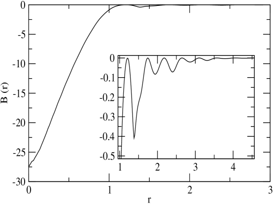
Figure 2: Bridge function $B_{0}(r)$ for n=3 at $\gamma=4.30$. The distance $r$ is in units of $a_{0}={(1/\rho)}^{1/2}$. Inset magnifies the values of $B_{0}(r)$ for $r\geq 1$.

with $s$=2 is used. The values of $B_{0}(r)$ are found by solving Eqs.(3.10)-(3.12) self-consistently. The value of $B_{0}(r)$ as a function of r for n= 3 is plotted in Fig. 2. The nature of $B_{0}(r)$ is same as was found in case of three-dimensions [27]. This value of $B_{0}(r)$ found for the reference potentials is used in relation (3.6) which is used to solve the OZ equation self-consistently to get values of ${h^{(0)}}(r)$ and ${c^{(0)}}(r)$. The values of ${\widehat{c}^{(0)}}(q)$ found by this method are shown in Fig. 1 by full lines. These values are close to the simulation values given by van Teeffelen et.al [20,21] for n=3. For n=6 and 12 values found from the RY closure and values found from the KR method are close showing that for short-range repulsive potentials the RY closure yields good values of pair correlation functions.

III.3 Calculation of $c^{(b)}({\bf r}_{1},{\bf r}_{2})$

For a crystal $c^{(b)}({\bf r}_{1},{\bf r}_{2})$ is invariant only under discrete set of translations corresponding to lattice vectors $\{\bf{R_{n}}\}$. If one chooses a center of mass variable ${\bf r}_{c}=\frac{({\bf r}_{1}+{\bf r}_{2})}{2}$ and difference variable ${\bf r}={\bf r}_{2}-{\bf r}_{1}$, the $c^{(b)}$ can be written as [11,12]

$$c^{(b)}({\bf r}_{1},{\bf r}_{2})=\sum_{G}\exp(i{\bf{G}}.{\bf r}_{c})c^{(G)}({\bf r};[\rho]),\hskip 113.81102pt(3.13)$$

where G are RLV’s. Since $c^{(b)}$ is real and symmetric with respect to interchange of ${\bf r}_{1}$ and ${\bf r}_{2}$ , $c^{(G)}({\bf r})=c^{(-G)}({\bf r})$ and $c^{(G)}({\bf r})=c^{(G)}(-{\bf r})$. The function $c^{(b)}({\bf r}_{1},{\bf r}_{2})$ can be expanded in terms of higher body direct correlation functions of uniform liquid [2];

$$c^{(b)}({\bf r}_{1},{\bf r}_{2};[\rho])=\int d{\bf r}_{3}{c_{3}}^{(0)}({\bf r}_{1},{\bf r}_{2},{\bf r}_{3};\rho_{0})(\rho({\bf r}_{3})-\rho_{0})\hskip 184.9429pt$$

$$+{\frac{1}{2}}\int d{\bf r}_{3}d{\bf r}_{4}{c_{4}}^{(0)}({\bf r}_{1},{\bf r}_{2},{\bf r}_{3},{\bf r}_{4};\rho_{0})(\rho({\bf r}_{3})-\rho_{0})(\rho({\bf r}_{4})-\rho_{0})+\cdots,\hskip 28.45274pt(3.14)$$

where $\rho({\bf r}_{n})-\rho_{0}=\sum_{G}\rho_{G}e^{i\bf{G}.{\bf r}_{n}}$, and ${c_{n}}^{(0)}$ are the n-body direct correlation functions of a uniform liquid of density $\rho_{0}$. These correlation functions are related to derivatives of $c^{(0)}(r,\rho_{0})$ with respect to density $\rho_{0}$ as follows [2] ;

$$\frac{\partial c^{(0)}(r)}{\partial\rho_{0}}=\int d{\bf r}_{3}{c_{3}}^{(0)}({\bf r}_{1},{\bf r}_{2},{\bf r}_{3}),\hskip 99.58464pt$$

$$\frac{\partial^{2}c^{(0)}(r)}{\partial{\rho_{0}}^{2}}=\int d{\bf r}_{3}\int d{\bf r}_{4}{c_{4}}^{(0)}({\bf r}_{1},{\bf r}_{2},{\bf r}_{3},{\bf r}_{4}),\hskip 28.45274pt(3.15)$$

etc.
The values of derivatives of $c^{(0)}(r)$ appearing on the left hand side of above equations can be found using the integral equation theory described above. The usefulness of this method to find $c^{(b)}({\bf r}_{1},{\bf r}_{2})$ depends on convergence of series Eq. $(3.14)$ which is a series in ascending powers of order parameters, and our ability of finding values of n-body $(n\geq 3)$ direct correlation functions from Eq. $(3.15)$. Barrat et.al [8] have shown that ${c_{3}}^{(0)}$ can be factored as ${c_{3}}^{(0)}({\bf r}_{1},{\bf r}_{2},{\bf r}_{3})=t(r_{12})t(r_{13})t(r_{23})$ and the function t(r) can be determined from relation (see Eq. $(3.15)$)

$$\frac{\partial c^{(0)}(r)}{\partial\rho_{0}}=t(r)\int d{\bf r}^{{}^{\prime}}t(r^{{}^{\prime}})t(|{\bf r}^{{}^{\prime}}-{\bf r}|).\hskip 56.9055pt(3.16)$$

This method can be extended for higher ${c_{n}}^{(0)}$ [29]. Since $\overline{c}^{(b)}({\bf r}_{1},{\bf r}_{2})$ is averaged over density $\rho$ and over order parameters $\rho_{G}$ the contributions made by successive terms of Eq. $(3.14)$ in ${A_{ex}}^{(b)}[\rho]$ is expected to decrease rapidly [11]. In the case of three dimensions it was found that it is only first term of the series $(3.14)$ which needs to be considered to describe accurately the fluid -solid transition [11, 29]. In two-dimensions the convergence is expected to be faster as number of nearest neighbours is less compared to the three-dimensions and therefore the higher body correlation functions expected to be less important. In view of this, we consider here the first term of the series $(3.14)$ only and examine its contribution in stabilizing the hexagonal lattice at the transition point.

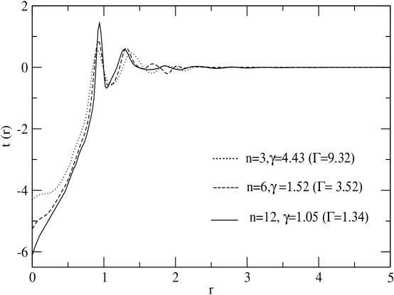
Figure 3: Function t(r) vs r for n=3, 6 and 12 at the values of $\gamma$ above the fluid-solid transition point, r is in units of $a_{0}=\left({1}/{\rho}\right)^{1/2}$.

From known values of $\frac{\partial c^{{}^{(0)}(r)}}{\partial\rho}$ we solved numerically Eq. $(3.16)$ to find values of t(r) for different values of $\gamma$. In Fig. 3, we plot values of t(r) for n = $3,6$ and $12$ at values of $\gamma$ close to the freezing point.
Taking only the first term of Eq. $(3.14)$ the expression for $c^{(b)}({\bf r}_{1},{\bf r}_{2})$ in terms of t(r) can be written as

$$c^{(b)}({\bf r}_{1},{\bf r}_{2})=\rho_{0}\sum_{G}\int d{\bf r}_{3}t(|{\bf r}_{3}-{\bf r}_{1}|){e^{i\bf{G}.{\bf r}_{3}}}t(|{\bf r}_{3}-{\bf r}_{2}|).\hskip 56.9055pt(3.17)$$

Using the relation

$${\bf r}_{3}=\frac{1}{2}{({\bf r}_{1}+{\bf r}_{2})}+({\bf r}_{3}-{\bf r}_{1})-\frac{1}{2}({\bf r}_{2}-{\bf r}_{1})$$

$$={\bf r}_{c}+{\bf r}^{{}^{\prime}}-\frac{1}{2}({\bf r}_{2}-{\bf r}),\hskip 73.97733pt$$

Eq. $(3.17)$ reduces to Eq. $(3.13)$, i.e.

$$c^{(b)}({\bf r}_{1},{\bf r}_{2})=\sum_{G}e^{i\bf{G}.{\bf r}_{c}}c^{(G)}({\bf r}),$$

where

$$c^{(G)}({\bf r})=\rho_{0}\mu_{G}t(r)e^{-\frac{1}{2}i\bf{G}.{\bf r}}\int d{\bf r}^{{}^{\prime}}t(r^{{}^{\prime}})e^{i\bf{G}.{\bf r}^{{}^{\prime}}}t(|{\bf r}^{{}^{\prime}}-{\bf r}|).\hskip 56.9055pt(3.18)$$

Using the relation $e^{i\bf{G}.{\bf r}}=\sum_{m}(i)^{m}J_{m}(Gr)e^{im(\phi_{G}-\phi_{r})}$ where $J_{m}(Gr)$ is the Bessel function of the first kind of integral order m we find following expression for $c^{(G)}(r)$;

$$c^{(G)}(r)=\sum_{M}(i)^{M}{c_{M}}^{(G)}(r)e^{-iM\phi_{r}},\hskip 142.26378pt(3.19)$$

where

$${c_{M}}^{(G)}(r)=\rho_{0}\mu_{G}t(r)\sum_{m}B_{m}(r,G)J_{m+M}{\left(\frac{1}{2}Gr\right)}e^{iM\phi_{G}}\hskip 56.9055pt(3.20)$$

and

$$B_{m}(r,G)=\int dkkt(k)J_{m}(kr)e^{im\phi_{r}}\int dr^{{}^{\prime}}r^{{}^{\prime}}J_{m}(kr^{{}^{\prime}})J_{m}(Gr^{{}^{\prime}})\hskip 42.67912pt(3.21)$$

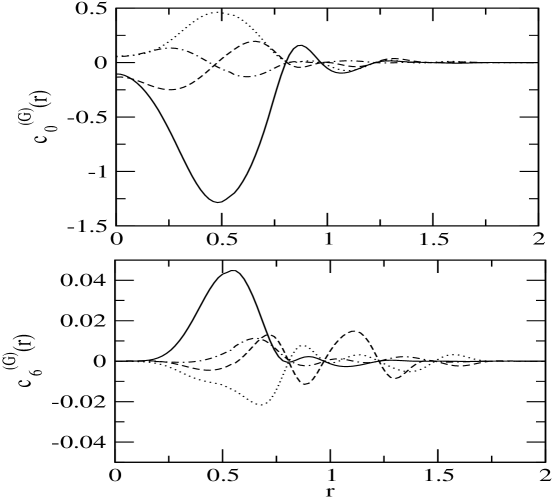
Figure 4: Harmonic coefficients ${c_{M}}^{(G)}(r)$ for RLV’s of first four sets for n=3, $\gamma=4.42(\Gamma=9.32)$. Notations are as follow: Full line represents values of the first set, the dotted line of the second set , dashed line of the third set and dashed-dotted line of the fourth set. The distance r is expressed in unit $a_{0}$, where $a_{0}(={{1}/{\rho}})^{{1}/{2}}$.

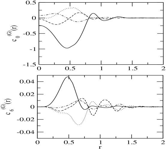
Figure 5: Harmonic coefficients ${c_{M}}^{(G)}(r)$ for RLV’s of first four sets for n=6, $\gamma=1.52(\Gamma=3.52)$. Notations are same as in Fig 4.

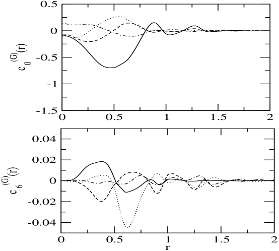
Figure 6: Harmonic coefficients ${c_{M}}^{(G)}(r)$ for RLV’s of first four sets for n=12, $\gamma=1.05(\Gamma=1.34)$. Notations are same as in Fig 4.

For hexagonal lattice $M=0,\pm 6$. The value of ${c_{M}}^{(G)}(r)$ depends on values of order parameters $\mu_{G}$ and on the values of RLV’s. In Figs. 4-6, we plot harmonic coefficients ${c_{0}}^{(G)}(r)$ and ${c_{6}}^{(G)}(r)$ for $n=3,6$ and $12$ for RLV’s of first four sets, respectively. For different set of RLV’s ${c_{M}}^{(G)}(r)$ varies with r in different way; the values in all cases become negligible for r ( measured in units of $a_{0}={(1/\rho)}^{1/2}$)$>1.5$ . For any given value of G, the values of ${c_{0}}^{(G)}(r)$ is about an order of magnitude larger than ${c_{6}}^{(G)}(r)$ at their maxima and minima. As magnitude of G increases value of ${c_{M}}^{(G)}(r)$ decreases and after the sixth set of RLV’s values of ${c_{M}}^{(G)}(r)$ become negligible for all values of n.

IV Liquid- Solid transition

Substituting expressions of $\rho(r)$ given by Eqs. $(2.17)$ and $(2.18)$ and of $\overline{c}^{(b)}({\bf r}_{1},{\bf r}_{2})$ given by Eq. $(3.19)$ in Eq. $(2.14)$ we find.

$$\frac{\Delta W}{N}=\frac{\Delta W_{id}}{N}+\frac{\Delta W_{0}}{N}+\frac{\Delta W_{b}}{N},\hskip 85.35826pt(4.1)$$

where

$$\frac{\Delta W_{id}}{N}=(1+\Delta\gamma)[1+\ln\left(\frac{\alpha}{\pi}\right)-2-\ln\rho_{0}]+1,\hskip 28.45274pt(4.2)$$

$$\frac{\Delta W_{0}}{N}=-\frac{1}{2}\Delta{\gamma}c^{(0)}(0)-\frac{1}{2}\sum_{G\neq 0}{|\mu_{G}|}^{2}\widehat{c}^{(0)}(G),\hskip 42.67912pt(4.3)$$

$$\frac{\Delta W_{b}}{N}=-\frac{1}{2}\sum_{G}{\sum_{G_{1}}}^{{}^{\prime}}\mu_{G_{1}}\mu_{-G-G_{1}}\hat{\overline{c}}({\bf{G}_{1}+\frac{1}{2}\bf{G}}).\hskip 42.67912pt(4.4)$$

where $\Delta\gamma=\left(\frac{\gamma_{s}-\gamma_{l}}{\gamma_{l}}\right)$ ; the subscripts s and l represent solid and liquid respectively.

Hear $\Delta W_{id},\Delta W_{0}$ and $\Delta W_{b}$ are respectively, the ideal, symmetry-conserving and symmetry-broken contributions to $\Delta W$. The prime on a summation in Eq $(4.4)$ indicates the condition ${\bf{G}}\neq 0,{\bf{G}}_{1}\neq 0$ and ${\bf{G}}+{\bf{G}}_{1}\neq 0$, and

$$\hat{c}^{(0)}(G)=\int c^{(0)}(r)e^{i\bf{G}.{\bf r}}d{\bf r}\hskip 56.9055pt$$

$$\hat{\overline{c}}({\bf{G}_{1}+\frac{1}{2}\bf{G}})=\int\overline{c}^{(G)}(r;\rho_{0})e^{-i({\bf{G}_{1}+\frac{1}{2}\bf{G})}.{{\bf r}}}d{\bf r}$$

We used above expressions to locate the liquid-crystal (hexagonal lattice) transition by varying values of $\gamma,\Delta\gamma$ and $\alpha$. The results given in Table 1 for n= $3,6$ and $12$ correspond to the RY closure relation. We note that the contribution arising due to symmetry broken part of the DPCF is far from negligible and its importance increases with the softness of potential. While it is about 7.3 $\%$ to the symmetry conserving term for n=12, it increases about 44 $\%$ for n=3. This explains why the Ramakrishnan-Yussouff theory gives good results for hard core potentials but fails for potentials that have soft core and/or attractive tail. As the contribution of $\frac{\Delta W_{b}}{N}$ is negative, it stabilizes the solid phase. Without it the theory strongly overestimates the stability of fluid phase specially for softer potentials [20,21]. The contribution made by the symmetry broken part of the DPCF is, as expected, small compered to that in three-dimensions (3D) at the freezing point for the same potential. For example, the contribution in 3D [11] for n=12 is 22.2 $\%$ compared to 7.3 $\%$ in 2D whereas for n=6 the contribution is 37 $\%$ in 3D and 18 $\%$ in 2D .

In Table 2 we compare results of the present calculation using both the RY closure and the KR procedure to calculate pair correlation functions for n=3 with the results found from other free-energy functionals as reported in ref $[21]$. The experimental results obtained from real-space microscopy measurements of magnetic colloids confined to an air-water interface [13] and values found from numerical simulations [30,31] are also given in the table. While the RY closure gives slightly higher values of $\Gamma_{f}$ and $\Gamma_{s}$ compared to experimental values, the KR closure gives slightly lower values. But these values along with the values of other parameters, particularly the values of $\Delta\Gamma=\Gamma_{s}-\Gamma_{f}$, are in better agreement with the experimental values compared to any other versions of the DFT. Although the extended modified weighted-density approximation (EMA) [32] with Verlet closure [33] gives values of $\Gamma_{f}$ which is close to the one found by us using the KR closure, but the values of $\Delta\Gamma$ is significantly lower; $\Delta{\Gamma}_{EMA}=0.16$ compared to the values found by us $\Delta\Gamma=0.41$, and the experimental value, $0.75$ .

The real-space experimental data are not available for other systems. The computer simulation results [34, 35] show the liquid-solid transition at $\gamma_{l}=1.51$ and $0.986$ respectively for $n=6$ and $12$. These values are close to the one given in Table 1.

V Summery and Perspectives

We used a free energy functional that contains both the symmetry-conserving part of the DPCF $c^{(0)}(r)$ and the symmetry-broken part $c^{(b)}({\bf r}_{1},{\bf r}_{2})$ to investigate the freezing of a two-dimensional fluid into a two-dimensional crystal of hexagonal lattice. The values of $c^{(0)}(r)$ and its derivatives with respect to density $\rho$ as a function of interparticle separation r have been determined using an integral equation theory comprising the OZ equation and the closure relations of Roger and Young [26] and of Kang and Ree [27]. For soft potential (n=3) the two results are found to differ; the KR closure seems to give better result. For more repulsive potentials the two results are close as shown in Fig. 1. For $c^{(b)}({\bf r}_{1},{\bf r}_{2})$ which is functional of $\rho({\bf r})$ and is invariant only under discrete set of translations and rotations, we used an expansion in ascending powers of order parameters. This expansion involves higher body direct correlation functions of isotropic phase, which in turn were found from the density derivatives of $c^{(0)}(r)$ using a method proposed by Barrat et.al [8].

The contribution of symmetry-broken part of DPCF to the free energy is found to depend on nature of pair potentials; the contribution increases with softness of potentials. This result is in agreement with that found in three-dimensions and explains why the Ramakrishnan-Yussouff free-energy functional was found to give a reasonably good description of the freezing transition of hard core potentials but failed for potentials that have soft core and/or attractive tail. The results found here and the results reported for 3D indicate that the theory described here can be used to investigate the freezing transitions of all kinds of fluids.

Since our free energy functional takes into account the spontaneous symmetry breaking it can be used to study various phenomena of ordered phases. The results indicate that the density-functional approach provides an effective frame work for theoretical study of a large variety of problems involving inhomogeneities. However, the question not adequately addressed yet is the size of fluctuations effect which play important role in two-dimensional systems. The other important question is the inclusion of hexatic phase in the theory.

Acknowledgments: We are thankful to J. Ram for computational help. One of us (Anubha) is thankful to the University Grants Commission for research fellowship.

Table 1. Freezing parameters $\alpha,\gamma_{l},\Delta\gamma$ and the pressure P at coexistence along with the contributions of ideal, symmetry-conserving and symmetry-broken parts of $\frac{\Delta W}{N}$. These results correspond to the Roger-Young closure [26].

n	$\alpha$	$\gamma_{l}$	$\Delta\gamma$	$\frac{\Delta W_{id}}{N}$	$\frac{\Delta W_{0}}{N}$	$\frac{\Delta W_{b}}{N}$	$\frac{\beta P}{\rho}$
3	100	4.96	0.025	2.50	-1.74	- 0.76	75
6	100	1.55	0.040	2.50	-2.10	- 0.40	31
12	96	1.00	0.050	2.49	-2.32	- 0.17	22

Table 2. Freezing parameters $\Gamma_{f}(={\gamma_{f}}^{n/2})$, $\Gamma_{s}(={\gamma_{s}}^{n/2})$ and the width of coexistence region $\Delta\Gamma=\Gamma_{s}-\Gamma_{f}$, and the relative displacement parameter $\xi(\simeq 2/\alpha)$ at the coexistence obtained from various density functional schemes. The MWDA stands for modified weighted density approximation, EMA for extended modified weighted density approximation, RY and KR refer to, respectively, the Roger-Young closure [26] and the Kang and Ree [27] closure.

	$\Gamma_{l}$	$\Gamma_{s}$	$\Delta\Gamma$	$\xi$
Present result with RY	11.04	11.46	0.42	0.020
Present result with KR	9.20	9.61	0.41	0.022
MWDA with RY [21]	41.07	41.13	0.06	0.017
EMA with RY [21]	23.00	23.08	0.09	0.020
EMA with Verlet [21]	9.33	9.49	0.16	0.020
Simulation [31]	12.0	12.25	0.025	-
Experiment [13]	10.0	10.75	0.75	0.038

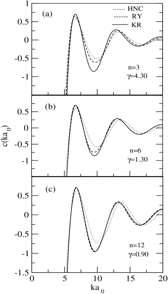
Figure 1: The dimensionless Fourier transform $\hat{c}^{(0)}(q)$ of the direct pair correlation function of ${c}^{(0)}(r)$ plotted against $ka_{0}\left(a_{0}=\left(1/\rho\right)^{1/2}\right)$ shown are data found from the integral equation theory using the RY closure (dashed line), HNC closure (dotted line) and KR closure (full line) at values of $\gamma$ shown in figure (a), (b) and (c) for n=3, 6 and 12, respectively.

.

References

- (1) P. M. Chaikin and T. C. Lubensky, Principles of Condensed Matter Physics (Cambridge University Press, 1995)
- (2) Y. Singh, Phys. Rep. 207, 351 (1991)
- (3) H. Lowen, Phys. Rep. 237, 249 (1994)
- (4) T. V. Ramakrishnan and M. Yussouff, Phys. Rev. B 19, 2775 (1979)
- (5) A. D. J. Haymet and D. W. Oxtoby, J. Chem. Phys. 74, 2559 (1981)
- (6) A. R. Denton and N. W. Ashcroft, Phys. Rev. A 39, 4701 (1989)
- (7) A. Khein and N. W. Ashcroft, Phys. Rev. Lett. 78, 3346 (1997)
- (8) J. L. Barrat, J. P. Hansen and G. Pastore, Mol. Phys. 63, 747 (1988)
- (9) W. A. Curtin, J. Chem. Phys. 88, 7050 (1988)
-
(10)
P. Mishra and Y. Singh, Phys. Rev. Lett. 97, 177801 (2006);
P. Mishra, S. L. Singh, J. Ram and Y. Singh, J. Chem. Phys. 127, 044905 (2007) - (11) S. L. Singh and Y. Singh, Europhys. Lett. 88, 16005 (2009)
- (12) S. L. Singh, A. S. Bharadwaj and Y. Singh, Phys. Rev. E 83, 051506 (2011)
-
(13)
K. Zahn, R. Lenke and G. Maret, Phys. Rev. Lett. 82, 2721 (1999) ;
H. H. von Grunberg, P. Keim, K. Zahn and G. Maret, Phys. Rev. Lett. 93, 255703 (2004) - (14) S. Z. Lin, B. Zheng and S. Trimper, Phys. Rev. E 73, 066106 (2006)
- (15) Y. Han, N. Y. Ha, A. M. Alsayed and A. G. Yodh, Phys. Rev. E 77, 041406 (2008)
- (16) T. V. Ramakrishnan, Phys. Rev. Lett. 48, 541 (1982)
- (17) X. C. Zeng and D. W. Oxtoby, J. Chem. Phys. 93, 2692 (1990)
- (18) J. C. Barrat, H. Xu, J. P. Hansen and M. Baus, J. Phys. C. 21, 3165 (1988)
- (19) V. N. Ryzhov and E. E. Tareyeva, Phys. Rev. B 51, 8789 (1995)
- (20) S. van Teeffelen, C. N. Likos, N. Hoffmann and H. Lowen Europhys. Lett. 75, 583 (2006)
- (21) S. van Teeffelen, H. Lowen and C. N. Likos, J. Phys. Condens. Matter 20, 404217 (2008)
- (22) E. P. Bernard and W. Krauth, Phys. Rev. Lett. 107, 155704 (2011).
-
(23)
B. I. Halperin and D. R. Nelson, Phys. Rev. Lett. 41,121 (1978);
D. R. Nelson and B. I. Halperin, Phys. Rev. B 19, 2457 (1979) - (24) A. P. Young, Phys. Rev. B 19, 1855 (1979).
- (25) J. P. Hansen and I. R. McDonald, Theory of Simple Liquids, 3rd ed (Academic press, Boston, 2006).
- (26) F. J. Rogers and D. A. Young, Phys. Rev. A 30, 999 (1984).
- (27) H. S. Kang and F. H. Ree, J. Chem. Phys. 103, 3629 (1995)
- (28) G. A. Martynov and G. Sarkisov, Mol. Phys. 49, 1495 (1983)
- (29) A. S. Bharadwaj and Y. Singh, unpublised
- (30) H Lowen, Phys. Rev. E 53, R29 (1996)
- (31) R. Haghgooie and P. S. Doyle, Phys. Rev. E 72, 011405 (2005)
- (32) C. N. Likos and N. W. Ashcroft, Phys. Rev. Lett. 69, 316 (1992); J. Chem. Phys. 99, 9090 (1993)
- (33) L. Verlet, Phys. Rev. 165, 201 (1968)
- (34) J. Q. Broughton, G. H. Gilmer and J. D. Weeks, Phys. Rev. B 25, 4651 (1982)
- (35) M. P. Allen, D. Frenkel, W. Gignac and J. P. McTague, J. Chem. Phys. 78, 4206 (1983)