Abstract

We present a new volatility model, simple to implement, that includes a leverage effect whose return-volatility correlation function fits to empirical observations. This model is able to capture both the “retarded effect” induced by the specific risk, and the “panic effect”, which occurs whenever systematic risk becomes the dominant factor. Consequently, in contrast to a GARCH model and a standard volatility estimate from the squared returns, this new model is as reactive as the implied volatility: the model adjusts itself in an instantaneous way to each variation of the single stock price or the stock index price and the adjustment is highly correlated to implied volatility changes. We also test the reactivity of our model using extreme events taken from the 470 most liquid European stocks over the last decade. We show that the reactive volatility model is more robust to extreme events, and it allows for the identification of precursors and replicas of extreme events.
Key Words: Volatility, tail event, risk management, asset pricing
JEL Classification: C5, G01, G1, G32

1 Introduction

Stylized facts from the financial markets include heavy tails, extreme correlation and leverage effect (Bouchaud and Potters, 2000, 2001; Cont, 2001). Various studies suggest that the power law nature of financial returns, ${\mathbb{P}}\{|r|>x\}\propto x^{-\alpha}$ (at large $x$) with a quasi-universal exponent $\alpha$ close to $3$, explains most extreme events, including crashes (Gabaix, Gopikrishnan, Plerou and Stanley, 2003). All these extreme events in the time series affect the estimation of the tail dependence measure (Davis and Mikosch, 2009). In particular, when the market is facing extreme negative returns, the level of correlation is significantly higher than during extreme positive returns (Longin and Solnik, 2001; Ang and Bekaert, 2002). This pattern can be explained by the asymmetry of volatility that is partly due to the so-called “leverage effect”. The leverage effect is characterized by a surge in volatility and a subsequent drop in the stock price (Black, 1976; Christie, 1982; Campbell and Hentchel, 1992; Bekaert and Wu, 2000).

The leverage effect puzzle is well documented in recent literature (Perello and Masoliver, 2003; Bollerslev, Litvinova and Tauchen, 2006; Qiu, Zheng, Ren and Trimper, 2006; Cevdet, Gallmeyer and Hollifield, 2007; Aït-Sahalia, Fan and Li, 2013). Various approaches have been suggested to include the leverage effect.

Continuous-time models. The Constant Elasticity of Variance model (CEV) developed by Cox (1975) is the first model that explicitly describes the relation between volatility and price. The elasticity stock price exponent allows the instantaneous variance of the percentage price change to be a direct inverse function of the stock price. Harvey and Shephard (1996) developed a stochastic volatility model with leverage effect to be estimated by a quasi-maximum likelihood procedure. Hagan, Kumar, Lesniewski and Woodward (2000) proposed a generalization of the CEV dynamics known as the SABR model. Carr and Wu (2009) proposed to model the equity-to-asset ratio by a simple CEV process in which large discontinuous shocks are modeled as a jump process to capture a self-exciting behavior. Veraart and Veraart (2009) modeled the leverage effect as a stochastic process by introducing an additional source of randomness into the stochastic volatility model. More recently, Filimonov and Sornette (2011) developed a model describing critical events in the self-organized systems such as financial markets. It relies on a self-excited multifractal process with an explicit dependence of the dynamics of the process on both external events and internal memory. It allows for leverage effect as an intrinsic property.

Discrete-time models. In the ARCH literature, the conditional variance is specified to be a function of the size and the sign of returns. One can mention the Exponential-GARCH (Nelson, 1991), the GJR-GARCH (Glosten, Jagannanthan and Runkle, 1993), the Asymmetric Power-ARCH (Ding, Granger and Engle, 1993), Nonlinear-GARCH (Engle and Ng, 1993) and the Threshold-GARCH (Zakoïan, 1994).

To our knowledge, both the continuous-time and discrete-time approaches remain focused mainly on theoretical issues. Bouchaud, Matacz and Potters (2001) are the first to study in detail the dynamics of the leverage effect adapted to stocks and stock indices. In particular, they introduced and measured the “return-volatility correlation function” for stocks and indices (Fig. 1). They derived two different dynamics for the systematic and specific risk and found a moderate (strong) correlation with a decay period of 50 (10) days for individual stocks (indices). The correlations for indices are therefore stronger than that for stocks, despite the fact that a stock index is merely a portfolio of stocks. They argue that the leverage effect for stocks stems from a simple retarded effect, in which price variations are calibrated not on the instantaneous value of the price but on an exponential moving average of the price. Their retarded volatility model adequately represents the leverage effect for individual stocks, which are mainly characterized by idiosyncratic (or specific) risks. However, they recognize that it is no longer the case for stock indices, which are only characterized by systematic risk, whose leverage is driven by another phenomenon, the so-called “panic effect”. This panic effect is partly explained by an increase of correlation between single stocks (Reigneron, Allez and Bouchaud, 2011). In fact, a fast decline of the market leads to the panic of investors and to an increase of the systematic risk of each single stock which may become the dominant factor when the panic is extreme. As emphasized by Allez and Bouchaud (2011), “during large swings of the index, the market exposure of stocks becomes the dominant factor”.

Relying on the retarded volatility model by Bouchaud, Matacz and Potters (2001), we develop a new volatility model, simple to implement, that (i) conserves the retarded effect property and (ii) adequately extends the leverage effect from the specific single stock case to the systematic case of stock indices, taking into account the panic effect. This model is well suited not only for stock indices but also for single stocks, particularly in times of distress during which stocks are mainly affected by the systematic risk. This advantage enables the model to be as reactive as the implied volatilities, i.e. there is no delay between the implied volatility changes and our model: they remain highly correlated. This important property makes it different from most previously published theoretical models.

The reactivity of the model is first tested against the European volatility index V2X and is also compared with two classical models selected as benchmarks: the GARCH model and the standard volatility estimate based on the square root of the exponential moving average of squared returns. The comparison to the volatility index is chosen because volatility is not directly observable and market participants prefer using implied volatility indices as market volatility proxies. Thus, how well the model captures the dynamics of such a proxy may be an adequate gauge of quality.

The robustness of the model is then tested using extreme events. An empirical study is performed on the 470 most liquid European stocks over the last decade. We investigate extreme systematic and specific risks, which could be responsible for massive losses and are therefore important for investors. Our results suggest that the market shocks are better assimilated into the reactive volatility model.

The article is organized as follows. Section 2 describes the reactive volatility model. Section 3 analyzes the empirical robustness of the model near extreme events. Section 4 summarizes the main findings and provides some concluding remarks.

2 The reactive volatility model

The reactive volatility model takes into account two different dynamic features of the leverage effect: it models the panic effect related to the systematic risk and combines it with the retarded volatility model of Bouchaud, Matacz and Potters (2001) that accurately describes the slow dynamics of the leverage effect for the specific risk. We focus first on the stock index case since it allows us to introduce the model of the panic effect that governs the systematic risk. Second we treat the single stock case that combines both the specific and systematic risks. We show how the retarded volatility model is combined with the panic effect in order to model at the same time the leverage effect of the specific and systematic risks.

2.1 Model of the panic effect describing the systematic risk: the case of stock index

Let $I(t)$ be a stock index at equally spaced, discrete times $t$. It is well known that arithmetic returns, $\Delta I(t)/I(t)$, are heteroscedastic, partly due to price-volatility correlations. The goal is to define a convenient estimator, a level $L(t)$, of the stock index $I(t)$ such that the renormalized arithmetic returns, $\Delta I(t)/L(t)$, become more homoscedastic.

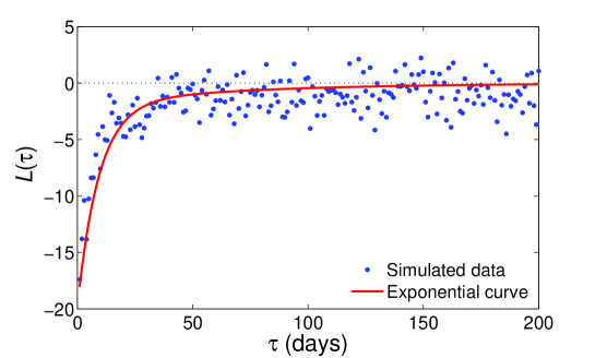
Figure 1: The return-volatility correlation function (leverage effect), ${\mathcal{L}}(\tau)\equiv\langle[\delta x(t+\tau)]^{2}\delta x(t)\rangle/\langle[\delta x(t)]^{2}\rangle^{2}$, with $\delta x(t)=\Delta I(t)/I(t)$, for simulated data (symbols), and the exponential curve ${\mathcal{L}}(\tau)\approx-A_{I}\exp(-\tau/T_{I})$, with $A_{I}=18$ and $T_{I}=9.3$ (days), as introduced and calibrated by Bouchaud, Matacz and Potters (2001). The simulated data are obtained from a Monte Carlo generated price series of 10,000 points, with $I(t+1)=I(t)(1+\sigma_{I}(t)\varepsilon_{t})$, in which i.i.d. $\varepsilon_{t}\sim{\mathcal{N}}(0,1)$, and $\sigma_{I}(t)$ is given by Eq. (7) with a constant $\tilde{\sigma}_{I}(t)=0.01$. This figure supports the claim that the reactive volatility model captures the leverage effect, using the correct parameters $A_{I}$ and $T_{I}$ calibrated from the empirical stock indices.

Let us introduce two stock index levels as exponential moving averages (EMAs) with two characteristic time scales: a slow level $L_{s}(t)$ and a fast level $L_{f}(t)$. These EMAs can be computed using standard linear relations:

$$L_{s}(t+1) = (1-\lambda_{s})L_{s}(t)+\lambda_{s}I(t+1)$$ (1)

$$L_{f}(t+1) = (1-\lambda_{f})L_{f}(t)+\lambda_{f}I(t+1)$$ (2)

where $\lambda_{s}$ and $\lambda_{f}$ are the weighting parameters of the EMAs. The appropriate values of $\lambda_{s}=0.0241$ and $\lambda_{f}=0.1484$ are extracted from the measurement of the return-volatility correlation function in Bouchaud, Matacz and Potters (2001), see the caption of Fig. 1 for details. The slow parameter corresponds to the relaxation time of the retarded effect for the specific risk whereas the fast one corresponds to the relaxation time of the panic effect for the systematic risk. These two relaxing times are found rather universal as they are stable in time and remain close to each other for different mature stock markets.

For practical purposes, a filter is introduced to make the estimator more robust against outliers or extreme instantaneous variations of the stock index. We set:

$$\hat{L}_{s}(t+1)=I(t+1)\left(1+F_{\phi}\left(\frac{L_{s}(t+1)-I(t+1)}{I(t+1)}\right)\right)$$ (3)

where a filter function $F_{\phi}(z)$ is proportional to $z$ for small $z$ and saturated to a constant for large $|z|$. We expect that the leverage effect is linear up to a certain point. We choose $\displaystyle F_{\phi}(z)=\frac{\tanh(\phi z)}{\phi}$, where $\phi$ is a parameter that determines the region of linearity of the filter, i.e., smaller $\phi$ correspond to wider linearity regions. At $\phi=0$, there is no filter, $F_{0}(z)=z$ and $\hat{L}_{s}(t+1)=L_{s}(t+1)$. This filter has only a very minor impact on the results and is useful in practice to level off a couple of very extreme events. One could use any other S-shaped function which is expected to give similar results. Finally, the main equation for the stock index level $L(t)$, in which the fast level is modulated by the filtered slow level, is defined as:

$$L(t+1)=\hat{L}_{s}(t+1)\left(1+F_{\phi}\left(\left(\frac{L_{f}(t+1)}{I(t+1)}\right)^{\ell}-1\right)\right)$$ (4)

where $\ell$ is the leverage parameter that describes the amplitude of the leverage effect between stock returns and volatility.

The leverage parameter $\ell$ is set to $8$ to reproduce the double exponential fit of the return-volatility correlation function in the stock index case (see the caption of Fig. 1 for details). For instance, the value of $\ell=8$ means that if the index varies by $1\%$, the volatility is expected to vary by $-\ell\cdot 1\%=-8\%$. That can be seen by using a Taylor expansion: if there is no filter ($\phi=0$) and $L_{f}(t+1)$ is close to $I(t+1)$, a Taylor expansion of Eq. (4) yields a simpler form:

$$L(t+1)\simeq\hat{L}_{s}(t+1)\left(1+\ell\leavevmode\nobreak\ \frac{L_{f}(t+1)-I(t+1)}{L_{f}(t+1)}\right)$$ (5)

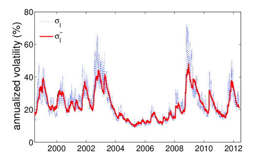
Figure 2: The measures of index volatility, $\sigma_{I}(t)$, from the reactive volatility model (dashed blue line) and the renormalized volatility $\tilde{\sigma}_{I}(t)$ (solid red line), for the period from 22/06/1998 to 18/05/2012. The renormalized volatility is less volatile in the short term but is able to capture all the long-term moves.

The Taylor expansion shows that the panic effect could be modeled in a simple way with two exponential moving averages whereas the retarded volatility model needs only one. The level $L(t)$ is the slow moving average of the retarded volatility model which is modulated by the relative excess of the systematic risk $I(t+1)$ as compared to its fast moving average $L_{f}(t+1)$. This modulation is amplified by the $\ell$ parameter which describes the “capacity” of the market to panic: $\ell=0$ corresponds to a market that never panics. It seems that the $\ell$ parameter is also universal as it is stable in time and is approximately the same for different mature stock markets.

The introduction of the leverage effect into Eq. (4) allows one to use the “corrected” level $L(t)$ instead of $I(t)$, which leads to more homoscedastic stock index returns $\Delta I(t)/L(t)$ than $\Delta I(t)/I(t)$, as tested below.

An estimator of the renormalized variance $\tilde{\sigma}_{I}^{2}$ is obtained through an EMA based on $L(t)$:

$$\tilde{\sigma}_{I}^{2}(t+1)=(1-\lambda_{\sigma})\tilde{\sigma}_{I}^{2}(t)+\lambda_{\sigma}\left(\frac{\Delta I(t+1)}{L(t+1)}\right)^{2}$$ (6)

where $\lambda_{\sigma}$ is a weighting parameter. $\lambda_{\sigma}$ has to be chosen as a compromise between the estimation accuracy of the standard deviation of the renormalized returns and the reactivity of that estimation. Indeed the renormalized returns are rather homoscedastic by construction in the short time scale only (in fact, the renormalization based on the leverage effect with short relaxation times ($\lambda_{s}$, $\lambda_{f}$) cannot account for long time scale changes of volatility related to economic cycles). Since economic uncertainty does not change significantly in a period of 2 months (40 trading days), we set $\lambda_{\sigma}$ to $1/40=0.025$. The related sample length leads to a noise of 4% in the annualized volatility which is in the order of 20%.

Figure 2 shows that $\tilde{\sigma}_{I}^{2}$ yields a stable output in the short time scale since the variation of the index $\Delta I(t+1)$ normalized by the index level $L(t+1)$ is rather homoscedastic by construction. The reactive volatility model is then obtained through this stable output but using a reactive renormalization factor. The reactivity of the model therefore comes from the renormalization factor $L(t+1)/I(t+1)$ that will adjust to every price move in an instantaneous way. The reactive volatility model $\sigma_{I}(t)$ for the systematic risk which is governed by the panic effect (the stock index case) is defined as:

$$\sigma_{I}(t+1)=\tilde{\sigma}_{I}(t+1)\frac{L(t+1)}{I(t+1)}$$ (7)

Using the Taylor expansion (5), we show that the normalization factor depends mainly on the slow and fast EMAs of the stock index price. The reactive volatility is therefore obtained by the following approximation:

$$\sigma_{I}(t+1)\approx\tilde{\sigma}_{I}(t+1)\frac{L_{s}(t+1)}{I(t+1)}\left(1+\ell\frac{L_{f}(t+1)-I(t+1)}{L_{f}(t+1)}\right)$$ (8)

2.2 Volatility term structure and the empirical test against the V2X index

We test the reactivity of Eq. (7) against the V2X implied volatility. Because the V2X index represents the implied volatilities of the Eurostoxx 50 index with a maturity $T$ of one month, one also needs to consider the volatility term structure of Eq. (7) which is defined as:

$$\sigma_{T}^{2}(t)=\frac{1}{T}\langle\left(\int_{t}^{T+t}\sigma_{I}^{2}(t^{\prime})dt^{\prime}\right)\rangle$$ (9)

where $\langle\ldots\rangle$ is the expectation (average) over all possible trajectories of $\sigma_{I}(t^{\prime})$ between $t$ and $t+T$.

In order to approximate $\sigma_{T}^{2}(t)$, one could have implemented a numerical solution based on Monte Carlo simulation (as described in the caption of Fig. 1). An alternative is to introduce an empirical recipe based on a two-factor model with the following two “long-term” volatilities, $\sigma_{Is}(t)$ (the slow factor) and $\sigma_{If}(t)$ (the fast factor). In this approximation, we assume the instantaneous volatility $\sigma_{I}(t)$ to mean-revert toward the fast “long-term” volatility $\sigma_{If}(t)$, which in turn mean-reverts toward the slow “long-term” volatility $\sigma_{Is}(t)$. The fast and slow “long-term” volatilities are defined as:

$$\sigma_{Is}(t)={\sigma}_{I}(t)\frac{I(t)}{L_{s}(t)}\qquad\sigma_{If}(t)={\sigma}_{I}(t)\frac{I(t)}{L_{f}(t)}$$ (10)

We split the squared volatility $\sigma_{I}^{2}(t)$ into three “components”:

$$\sigma_{I}^{2}(t)=({\sigma}_{I}^{2}(t)-{\sigma}_{If}^{2}(t))+({\sigma}_{If}^{2}(t)-{\sigma}_{Is}^{2}(t))+{\sigma}_{Is}^{2}(t)$$ (11)

The empirical observation from Fig. 3 confirms, without pretending to any rigor, that $(\sigma_{I}^{2}(t)-\sigma_{If}^{2}(t))$ and $(\sigma_{If}^{2}(t)-\sigma_{Is}^{2}(t))$ can be seen as two mean-reverting processes with two relaxation rates $\lambda_{s}$ and $\lambda_{f}$, while ${\sigma}_{Is}^{2}(t)$ varies much slower than the other processes. We therefore assume that $(\sigma_{I}^{2}(t)-\sigma_{If}^{2}(t))$ and $(\sigma_{If}^{2}(t)-\sigma_{Is}^{2}(t))$ can be approximated by Ornstein-Uhlenbeck processes with two relaxation rates $\lambda_{s}$ and $\lambda_{f}$, while ${\sigma}_{Is}^{2}(t)$ follows Brownian motion. These last assumptions (current in the literature, e.g., Hull and White (1987); Heston (1993)) enable the reactive volatility estimator with the term structure, $\sigma_{T}$, to be estimated as:

$$\sigma_{T}^{2}(t)\approx(\sigma_{I}^{2}(t)-\sigma_{If}^{2}(t))\frac{(1-e^{-\lambda_{f}T})}{\lambda_{f}T}+(\sigma_{If}^{2}(t)-{\sigma}_{Is}^{2}(t))\frac{(1-e^{-\lambda_{s}T})}{\lambda_{s}T}+\sigma_{Is}^{2}(t)$$ (12)

This relation can be seen alternatively as an empirical definition of $\sigma_{T}(t)$ or as a practical recipe for its computation.

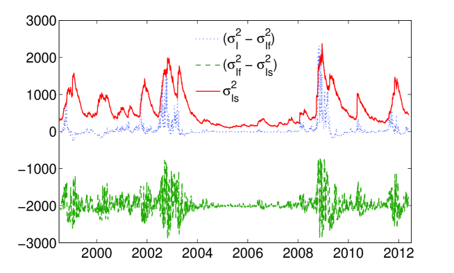
Figure 3: Empirical behavior of three “components” in Eq. (11): $(\sigma_{I}^{2}(t)-\sigma_{If}^{2}(t))$ (dotted blue line), $(\sigma_{If}^{2}(t)-\sigma_{Is}^{2}(t))$ (dashed green line, which is shifted by $-2000$ along the vertical axis), and ${\sigma}_{Is}^{2}(t)$ (solid red line). The first two components can be seen as mean-reverting processes with different relaxation rates, while the last varies much slower than the others.

Figure 4 compares the implied volatility V2X for Eurostoxx 50 to four different volatility estimators: (i) a standard estimator with an exponential moving average of squared returns:

$$\sigma_{I,SD}^{2}(t+1)=(1-\lambda_{\sigma})\sigma_{I,SD}^{2}(t)+\lambda_{\sigma}\left(\frac{\Delta I(t+1)}{I(t)}\right)^{2}$$ (13)

with the same value of the weighted parameter $\lambda_{\sigma}=1/40$; (ii) a GARCH estimator, $\sigma_{GARCH}(t)$, which is often considered to be the gold standard; (iii) the reactive volatility estimator $\sigma_{I}(t)$ from Eq. (7) without a term structure; and (iv) the reactive volatility estimator $\sigma_{T}(t)$ from Eq. (12) with the term structure. One can see that both the standard and GARCH estimators have much lower correlations with V2X than both reactive estimators. Additionally, the term structure model for the reactive volatility estimator, as expected, improves the slope of the linear regression. Indeed, the slope becomes much closer to $1$. The $R^{2}$ from the linear regression is relatively high (around $0.45$). We can therefore consider the model to be nearly as reactive as the volatility index.

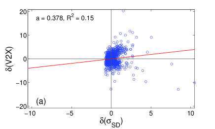
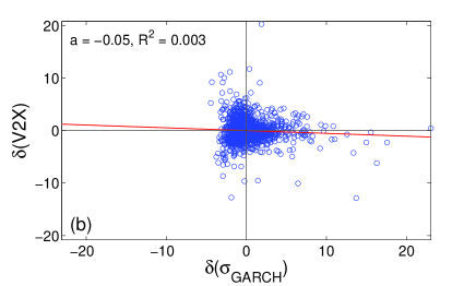
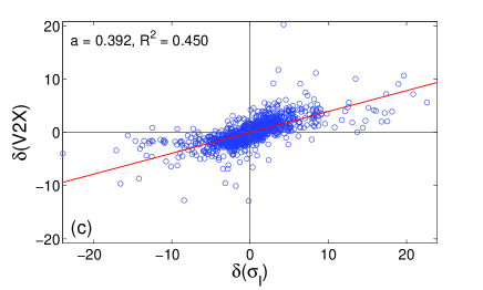
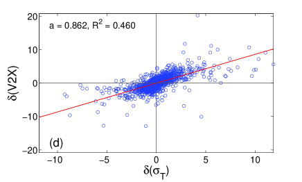
Figure 4: Correlations between increments $\delta(\rm{V2X})$ of the Eurostoxx 50 implied volatility index V2X (vertical axis) and increments of four different volatility estimators (horizontal axis): (a) a standard estimator based on the exponential moving average of the squared returns ($\lambda_{\sigma}=1/40$); (b) a standard GARCH estimator ($\omega=0.0000014$, $\alpha=0.1064523$, $\beta=0.8966662$); (c) the reactive volatility estimator without a term structure; and (d) the reactive volatility estimator with a term structure. First, the increments in volatility for both the standard volatility and GARCH estimators are much more strongly skewed towards positive values. Second, the correlations between the V2X and both reactive volatility estimators are much higher. Finally, accounting for the term volatility structure increases the slope of a linear regression from $0.392$ to $0.862$, with the latter value being close to $1$.

2.3 Model for combining panic and retarded effects: the case of single stock

For a single stock, the reactive volatility model relies on an equation similar to Eq. (7) used for the stock index:

$$\sigma_{i}(t+1)=\tilde{\sigma}_{i}(t+1)\frac{L_{i}(t+1)}{P_{i}(t+1)}$$ (14)

with $L_{i}(t+1)$ and $\tilde{\sigma}_{i}(t+1)$ obtained through equations similar to Eqs. (4, 6), respectively. The only difference comes from $\hat{L}_{s}(t+1)$ in Eq. (4), which applies now to the single stock price $P_{i}(t)$ instead of the index price $I(t)$. Using the Taylor expansion (5), we obtain:

$$\sigma_{i}(t+1)\approx\tilde{\sigma}_{i}(t+1)\frac{L_{i,s}(t+1)}{P_{i}(t+1)}\left(1+\ell\frac{L_{f}(t+1)-I(t+1)}{L_{f}(t+1)}\right)$$ (15)

This formula combines the slow EMA of the single stock price on one hand, and the fast EMA and the current price of the stock index, on the other hand. As a consequence, it adequately extends the leverage effect from the specific risk case (already accounted in the retarded volatility model), to the systematic case, which captures the panic effect. In what follows, the reactive volatility estimator $\sigma_{i}(t)$ from Eq. (14) is tested and used to identify precursors and replicas around extreme events.

Finally although the formula used to determine the level $L_{i}(t)$ for the single stock case looks similar to that used to determine the level $L(t)$ of the stock index, the leverage effect is different from a practical point of view. Indeed the leverage effect for the stock index depends only on the historical stock index price and is dominated by the fast panic effect; in turn, the leverage effect for a single stock depends on both the single stock price and the stock index price, and it is dominated by the slow retarded effect. However as soon as the systematic risk becomes dominant as compared to the specific risk (that happens when the market is highly stressed), the leverage effect in the single stock starts to be also dominated by the panic effect.

Our approach manages to combine the panic effect model introduced in Sect. 2.1 with the retarded volatility model by Bouchaud, Matacz and Potters (2001). This combination allows us to model the leverage effect for both the systematic and specific risks that occur in the single stock case. In that case the level $L(t)$ is that of the specific risk obtained with the retarded volatility model modulated by the panic effect in Eq. (5). The panic effect is correlated to the relative excess of the systematic risk with as compared to fast moving average.

The model manages to adjust its estimation of the volatility in a instantaneous way at each single stock or index price variation. Moreover, the adjustment is highly correlated to variations of the volatility index. One can expect that the model will manage to capture, in a reactive way, not only the risk of the stock index but also the systematic risk of any stock.

3 Empirical test of the reactive volatility model around extreme events

3.1 Data analysis

The database consists of daily price series for the 470 most liquid European stocks from January 1st 2000 to April 4th 2012. Let $P_{i}(t)$ denote the closing price of $i$-th stock at day $t$. From each price series, an array of arithmetic returns, $R_{i}(t)=\frac{P_{i}(t)-P_{i}(t-1)}{P_{i}(t-1)}$, is constructed. An extreme event is said to occur when the absolute arithmetic return $|R_{i}(t)|$ is three times larger than the reactive volatility estimator $\sigma_{i}(t-1)$:

$$|R_{i}(t)|>3\sigma_{i}(t-1)$$ (16)

For each stock, we search for extreme events in the array $\{R_{i}(t)\}$. At each occurrence of an extreme event, we record the subsequence $\{r(-\Delta),r(-\Delta+1),...,r(0),r(1),...,r(\Delta)\}$ of normalized returns before and after the extreme event (at day $t$),

$$r(k)=\frac{R_{i}(t+k)}{\sigma_{i}(t+k-1)}\qquad(k=-\Delta...\Delta)$$ (17)

where $\Delta$ is a fixed subsequence length with $\Delta=9$ trading days. The subsequence $\{r(k)\}$ characterizes the behavior of a stock before and after an extreme event, which is identified by the magnitude of $r(0)$ (we drop the index $i$ because the extreme events will be analyzed for all stocks together). Repeating this procedure for each stock generates a database of 10,213 extreme events. Note that if two (or more) extreme events occurred within $\Delta$ days, only the first one is retained, while any later events are ignored. It is worth emphasizing that the above definition of an extreme event is purely conventional, as is the choice for the threshold $3\sigma_{i}(t-1)$. Note also that if stock returns were Gaussian, the number of extreme events would be much smaller than what we observe because the probability of a Gaussian return larger than $3\sigma$ is $0.0027$.

A closer look into the statistical properties of stock returns around extreme events requires distinguishing the systematic risk from the specific risk. The systematic risk mainly affects the stock indices (or even every stock during stress conditions), while the specific risk mainly affect single stocks. More precisely, the database records are split into four groups that are denoted “systematic positive” (SyP), “systematic negative” (SyN), “specific positive” (SpP) and “specific negative” (SpN). The division into positive and negative groups is determined by the sign of the extreme normalized return $r(0)$. The division into systematic and specific groups is decided by the condition on the Eurostoxx index $I(t)$ at the day $t$ of an extreme return: if $|\Delta I(t)|$ exceeds $3\%$, the extreme event is categorized as systematic, otherwise as specific. Both systematic groups (SyP & SyN) contain the records of extreme returns from individual stocks that are affected by large stock index returns, representing extreme events for the entire market. The specific groups (SpS & SpN) contain the records of extreme returns that are specific to individual stocks. The database of extreme events contains 903 systematic positive records, 1,046 systematic negative records, 5,135 specific positive records and 3,129 specific negative records.

To qualitatively separate the possible sources of deviations (accuracy of the reactive volatility estimator and return correlations), a second database of “non-extreme” events is constructed with the same structure, in which dates $t$ are chosen randomly (without the selective condition (16)). In this case, no strong correlations between successive returns are expected, and the reactive volatility estimator is expected to accurately capture the fluctuations of the stock price.

3.2 Empirical results

The behavior of the reactive volatility model around extreme events is characterized by the following function:

$$q_{k}=\sqrt{\langle r^{2}(k)\rangle}-1\qquad(k=-\Delta\ldots\Delta)$$ (18)

where the arithmetic average $\langle...\rangle$ is taken over all records in the chosen group (SyP, SyN, SpP, SpN). For the idealized case in which the returns are uncorrelated and the reactive volatility estimator $\sigma_{i}(t)$ is exact, the average $\langle r^{2}(k)\rangle$ of normalized returns should be equal to $1$, so that $q_{k}$ would be $0$, except for $k=0$. In other words, the smallness of deviations of $q_{k}$ from $0$ characterizes the accuracy of the volatility estimator.

Group	Before		After
	Standard	Reactive	Standard	Reactive
Systematic positive	0.76	0.34	0.52	0.35
Systematic negative	0.55	0.21	1.02	0.54
Specific positive	0.54	0.11	0.90	0.31
Specific negative	0.54	0.22	1.13	0.45

Table 1: The level of deviations $q_{k}$ is averaged over 9 days before and after an extreme event. For all groups of extreme events, this level is significantly higher for a standard volatility estimator than for the reactive volatility model because the latter captures the panic effect for the systematic groups and the retarded effect for the specific groups. Note also that the recovery after an extreme event takes, on average, $2.95$ days for the reactive volatility model, as opposed to $5.29$ days for a standard estimator (both times are estimated from an exponential fit of $q_{k}$ after an extreme event; see Fig. 5). As a consequence, the reactive volatility model is qualified as more robust in response to extreme events.

Table 1 summarizes the average characteristics obtained for both estimators. The level of deviations $q_{k}$ is averaged over 9 days before and after an extreme event, as illustrated in Figs. 5, 6. For all groups of extreme events, this level is significantly higher for the standard volatility estimator than for the reactive volatility model because the latter captures the panic effect for the systematic groups and the retarded effect for the specific groups. One can conclude that the reactive volatility model is more robust near extreme events, and its recovery after a shock is faster.

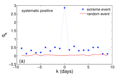
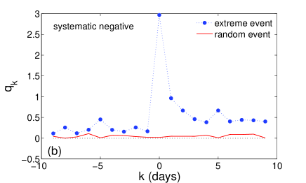
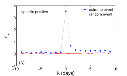
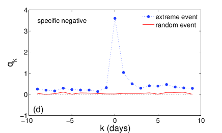
Figure 5: Distribution of $q_{k}$ around an extreme event for the reactive volatility model. Extreme returns are split into four groups: (a) SyP, (b) SyN, (c) SpP and (d) SpP. A stock return is termed extreme when it exceeds threefold the empirical volatility $\sigma_{i}(t-1)$ from the reactive volatility model. The selected interval is $\pm 9$ days.

Figure 5 shows $q_{k}$ for the four groups. Full circles represent $q_{k}$ from the database of extreme events, while the solid line is used as a reference level from the database of random events (extreme or not). The solid line is close to $0$, which indicates that the reactive volatility model is accurate for ordinary days (without extreme events). For comparison, Fig. 6 shows the quantities $q_{k}$ computed in Eq. (18) by replacing $\sigma_{i}(t)$ in Eq. (17) with an empirical measure of volatility, $\sigma_{i,SD}(t)$, which is obtained from a standard volatility estimator with an exponential moving average:

$$\sigma_{i,SD}^{2}(t+1)=(1-\lambda_{\sigma})\sigma_{i,SD}^{2}(t)+\lambda_{\sigma}[R_{i}(t+1)]^{2}$$ (19)

with the same value of the weighting parameter $\lambda_{\sigma}=1/40$.

Let us now take a closer look at the results of Fig. 5. For systematic groups, there are significant deviations of $q_{k}$ from $0$ before and after an extreme event. In other words, the normalized returns before and after an extreme event are significantly larger than typical normalized returns. Prior to an extreme event, the normalized returns increase very slowly and become significantly larger than typical normalized return 30 days before the event. The relaxation time after the extreme event is on contrary much faster.

In the systematic positive group, the observation of relatively strong precursors might be partly explained by political or monetary decisions made in reaction to earlier market instabilities.

For the systematic negative group, the observation of excitements before an extreme event is less intuitive. These variations could come from the possibility that some investors anticipate the release of very bad economic news earlier than others. After an extreme event, large renormalized returns are naturally expected as the market relaxes after this event. It means that investors should be worried about replicas after the initial extreme event and that most models consistently underestimate risk.

Figures 5c, 5d for both specific groups indicate less significant deviations of $q_{k}$ from $0$ before an extreme event.

In the specific positive group, the observation of an extreme positive return can be caused by announcements of corporate decisions (mergers or acquisitions). Because these corporate decisions remain strictly confidential and are difficult to anticipate, one expects to observe very weak precursors and small values of $q_{k}$ for negative $k$. After the day of announcement, the stock returns may experience a rapid relaxation (one or two days) towards the normal level of small $q_{k}$ for positive $k$.

For the specific negative group, the observation of an extreme event can be caused by an announcement of corporate decisions related to bad economic results for the company (profit warning, bankruptcy, or downgrade). This kind of news is partly anticipated by the market through rumors. One therefore can identify stronger precursors of extreme events. Because the situation of the company remains tenuous, stronger replicas are also identified.

The mechanisms of these precursors in every case seem plausible especially since the volatility forecasts are not particularly low when these relatively large events may happen. Indeed we compare the whole sample and the conditional sample defined by the days prior to any extreme event until 9 days. The average of the volatilities forecasted by our volatility model is $31\%$ in the conditional sample and remains close to that estimated for the whole sample ($33\%$). We also find similar results for the standard deviations of returns. We manage to identify statistically the presence of precursors of extreme events in each case, but the precursors remain too weak to be detected one by one to forecast the occurrence of an extreme event. Indeed the predictive power is low and the model cannot be used to forecast any crash or extreme event. For example, if a warning signal emerges each time the realized volatility exceeds twice the level predicted by the reactive volatility model for a period of 9 days, $96.68\%$ of the extreme events will be missed, while $56.8\%$ will be false warning signals.

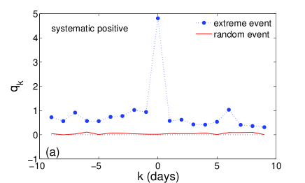
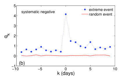
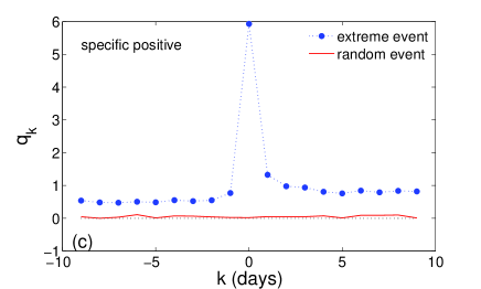
Figure 6: Distribution of $q_{k}$ around an extreme event for a standard volatility estimator. Extreme returns are split into four groups: (a) SyP, (b) SyN, (c) SpP and (d) SpN. A stock return is termed extreme when it exceeds threefold the empirical volatility $\sigma_{i,SD}(t-1)$ from a standard volatility estimator. The selected interval is $\pm 9$ days.

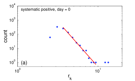
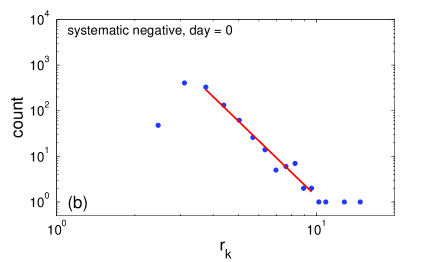
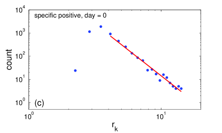
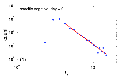
Figure 7: Asymptotic behavior of the probability density $p(z)$ of extreme returns normalized with the reactive volatility model

for the four groups: (a) SyP, (b) SyN, (c) SpP and (d) SpN. In all cases, power law decays $p(z)\propto z^{-1-\alpha}$ are observed, with the exponents $5.5$, $4.5$, $3.5$ and $3.2$ for the systematic positive, systematic negative, specific positive and specific negative groups, respectively. For the systematic groups, the exponent is greater than $4$, indicating the existence of kurtosis, while for the specific groups, the exponent is less than $4$.

Similar plots in Fig. 6 for a standard volatility estimator display a less reactive measure around extreme events.

Figure 7 shows the asymptotic behavior of the probability density $p(z)$ of extreme normalized returns for the four groups. In all cases, power law decays $z^{-1-\alpha}$ are observed, with the exponent $\alpha$ equal to 5.5, 4.5, 3.5 and 3.2 for the SyP, SyN, SpP and SpN groups, respectively. For the systematic groups, the exponent is greater than $4$, indicating the existence of kurtosis. The renormalization of returns with the reactive volatility model, instead of using the standard EMA volatility estimate, has managed to increase the exponent from $3$ to $5$, which means that this model is able to capture most of the extreme events. For the specific groups, the exponent remains around $3$. Most of these extreme risks come from very specific news (for example, a takeover offer), and most of the time, when the price jumps, the volatility does not change.

4 Conclusion

We developed a new volatility model, easy to implement, that includes a leverage effect whose return-volatility correlation function fits to empirical observations. In addition, the model is able to capture both the panic effect induced by the systematic risk and the retarded effect induced by the specific risk. The model is shown to be as reactive as the implied volatility, which is an improvement over other models. To test the robustness of the reactive volatility model near extreme events, an empirical study is performed on 470 the most liquid European stocks from January 1st 2000 to April 4th 2012. The reactive volatility model is used to renormalize daily returns, among which extreme events are identified and split into four groups: systematic positive, systematic negative, specific positive and specific negative. Our results suggest that the market shocks are better assimilated into the reactive volatility model. Moreover, the model identifies statistically the presence of precursors and replicas. The model captures much of the extreme systematic risk and a significant part of the extreme specific risk. Future research will include an application of the reactive volatility model to estimate market beta, the aggregation of risk and VaR of a Long/Short portfolio.

References

- Aït-Sahalia, Fan and Li (2013) Aït-Sahalia Y., J. Fan and Y. Li, The leverage effect puzzle: Disentangling sources of bias at high frequency. Working paper, Princeton University, 2013.
- Allez and Bouchaud (2011) Allez, R. and Bouchaud, J.P., Individual and collective stock dynamics: intra-day seasonalities. New Journal of Physics, 2011, 13, 025010.
- Ang and Bekaert (2002) Ang, A. and Bekaert, G., International asset allocation with regime shifts. Review of Financial Studies, 2002, 11, 1137-1187.
- Bekaert and Wu (2000) Bekaert, G. and Wu, G., Asymmetric volatility and risk in equity markets. Review of Financial Studies, 2000, 13, 1-42.
- Black (1976) Black, F., Studies in stock price volatility changes, American Statistical Association, Proceedings of the Business and Economic Statistics Section, 1976, 177-181.
- Bollerslev, Litvinova and Tauchen (2006) Bollerslev, T., J. Litvinova, and G. Tauchen, Leverage and volatility feedback effects in high-frequency data. Journal of Financial Econometrics, 2006, 4, 353-384.
- Bouchaud and Potters (2000) Bouchaud, J.-P. and Potters M., Theory of Finantial Risks: From Statistical Physics to Risk Management (Cambridge University Press 2000).
- Bouchaud and Potters (2001) Bouchaud, J.-P., and Potters, M., More stylized facts of financial markets: Leverage effect and downside correlations. Physica A, 2001, 299, 60-70.
- Bouchaud, Matacz and Potters (2001) Bouchaud, J.-P., Matacz, A., and Potters, M., Leverage effect in financial markets: The retarded volatility model. Physical Review Letters, 2001, 87, 1-4.
- Campbell and Hentchel (1992) Campbell, J. Y. and Hentchel, L, No news is good news: An asymmetric model of changing volatility in stock returns. Journal of Financial Economics, 1992, 31, 281-318.
- Carr and Wu (2009) Carr P. and L. Wu, Leverage effect, volatility feedback, and self-exciting market disruptions. Working paper, New York University, 2009.
- Cevdet, Gallmeyer and Hollifield (2007) Cevdet A., M. Gallmeyer and B. Hollifield, Financial leverage and the leverage effect - A market and firm analysis. Working paper, Carnegie Mellon University, 2007.
- Christie (1982) Christie, A., 1982, The stochastic behavior of common stock variances - value, leverage, and interest rate effects, Journal of Financial Economic Theory, 1992, 10, 407-432.
- Cont (2001) Cont, R., Empirical properties of asset returns: stylized facts and statistical issues. Quantitative Finance, 2001, 1, 223-236.
- Cox (1975) Cox, J., Notes on Option Pricing I: Constant elasticity of diffusions. Working paper, Stanford University, 1975.
- Davis and Mikosch (2009) Davis, R. and Mikosch, T., Extremogram: A correlogram for extreme events. Bernoulli, 2009, 15, 977-1009.
- Ding, Granger and Engle (1993) Ding, Z., C. Granger and R. Engle, A long memory property of stock market returns and a new model. Journal of Empirical Finance, 1993, 1, 83-106.
- Engle and Ng (1993) Engle, R. and Ng, V., Measuring and testing the impact of news in volatility. Journal of Finance, 1993, 43, 1749-1778.
- Filimonov and Sornette (2011) Filimonov V. and D. Sornette, Self-excited multifractal dynamics. Europhysics Letters, 2011, 94, 46003.
- Gabaix, Gopikrishnan, Plerou and Stanley (2003) Gabaix, X., Gopikrishnan, P., Plerou, V. and Stanley, E.H., A theory of power law distributions in financial market fluctuations. Nature, 2003, 423, 267-270.
- Glosten, Jagannanthan and Runkle (1993) Glosten, L.R., Jagannanthan, R., and Runkle, D., Relationship between the expected value and the volatility of the nominal excess return on stocks. Journal of Finance, 1993, 48, 1779-1802.
- Hagan, Kumar, Lesniewski and Woodward (2000) Hagan P., Kumar D., Lesniewski A.S. and Woodward D.E., Managing smile risk. Working paper, Bear Stearns, 2000.
- Harvey and Shephard (1996) Harvey, A. C. and N. Shephard, The estimation of an asymmetric stochastic volatility model for asset returns. Journal of Business and Economic Statistics, 1996, 14, 429-434.
- Heston (1993) Heston, S., A Closed-Form Solution for Options with Stochastic Volatility with Applications to Bond and Currency Options, Review of Financial Studies, 1993, 6, 327-343.
- Hull and White (1987) Hull, J., and A. White, The Pricing of Options On Assets With Stochastic Volatilities, Journal of Finance, 1987, 42, 281-300.
- Longin and Solnik (2001) Longin, F., and Solnik, B., Extreme correlation of international equity markets. Journal of Finance, 2001, 56, 649-676.
- Nelson (1991) Nelson, D., Conditional heteroskedasticity in asset pricing: a new approach. Econometrica, 1991, 59, 347-370.
- Perello and Masoliver (2003) Perello J. and J. Masoliver, Random diffusion and leverage effect in financial markets. Physical Review E, 2003, 67, 037102.
- Reigneron, Allez and Bouchaud (2011) Reigneron, P.A., Allez, R. and Bouchaud, J-P., Principal regression analysis and the index leverage effect. Physica A, 2011, 390, 3026-3035.
- Qiu, Zheng, Ren and Trimper (2006) Qiu T., B. Zheng, F. Ren and S. Trimper, Return-volatility correlation in financial dynamics. Physical Review E, 2006, 73, 0651031(4).
- Shen and Zheng (2009) Shen J. and B. Zheng, On return-volatility correlation in financial dynamics. Europhysics Letters, 2009, 88, 28003.
- Veraart and Veraart (2009) Veraart A.E.D. and A.M. Veraart, Stochastic volatility and stochastic leverage. Working paper, Aarhus University, 2009.
- Zakoïan (1994) Zakoïan, J.M., Threshold heteroskedastic models. Journal of Economic Dynamics and Control, 1994, 18, 931-955.