Eigenwaves in Waveguides with Dielectric Inclusions:

Spectrum

Y. Smirnov^a and Y. Shestopalov^b

^a Penza State University, Penza, 440017 Russia (smirnov@penzadom.ru)

^b Karlstad University, SE 65188 Karlstad, Sweden (youri.shestopalov@kau.se)

Abstract. We consider fundamental issues of the mathematical theory of the wave propagation in waveguides with inclusions. Analysis is performed in terms of a boundary eigenvalue problem for the Maxwell equations which is reduced to an eigenvalue problem for an operator pencil. We formulate the definition of eigenwaves and associated waves using the system of eigenvectors and associated vectors of the pencil and prove that the spectrum of normal waves forms a nonempty set of isolated points localized in a strip with at most finitely many real points.

Keywords: eigenwave; waveguide; pencil; spectrum; dielectric; inclusion

AMS Classification: 45E99, 31B20, 83C50, 74S10

1 Introduction

Analysis of the wave propagation in waveguides with nonhomogeneous filling and arbitrary inclusions (perfectly conducting and dielectric) constitutes an important class of vector electromagnetic problems. However, many urgent tasks here remain unsolved that have been known for empty waveguides since the late 1940s; namely: existence of normal waves and their basic properties including the discreteness and localization the spectrum of normal waves on the complex plane, completeness and basis property in terms of both longitudinal and transversal field components, and so on.

The theory of electromagnetic wave propagation in waveguides with homogeneous filling were elaborated in classical works of A.N. Tikhonov and A.A. Samarskii [40]–[42]. The analysis in this case is reduced to two scalar selfadjoint problems which are studied using standard methods. List the most important results obtained for homogeneous waveguides: there exists a (countable) set of eigenvalues (spectrum of normal waves of a waveguide) consisting of real isolated points with the only accumulation point at infinity and the system of normal waves is complete and forms a basis. For nonhomogeneous waveguides with given cross-sectional geometry, in particular, rectangular [52, 7] and circular [29], the results concerning existence and distribution of the normal wave spectra on the complex plane are obtained by reducing to explicit dispersion relations and analysis of the corresponding complex-valued functions of one or several complex variables.

To the best of our knowledge, the existence of eigenvalues and their distribution on the complex plane remain an open issue as well as the completeness and basis property for the system of normal waves in nonhomogeneously filled waveguides with arbitrary inclusions. This fact has become a main reason for us to complete in this paper the mathematical theory of wave propagation in waveguides by filling these gaps.

Let us briefly summarize the new fundamental results obtained in this study for an arbitrary waveguide with nonhomogeneous filling and arbitrary inclusions (that belongs to the considered family):

(i) the spectrum of normal waves is nonempty and forms a countable set of isolated points on the complex plane (cut along two intervals on the real axis) without finite accumulation points;

(ii) the spectrum is symmetric with respect to the axes on the complex plane, is localized in a strip, and contains not more than a finite number of real points.

During the last two decades an increasing interest has been reported to the study of electromagnetic wave propagation in guiding systems with nonhomogeneous filling. Different types of them have been created and found various practical applications and many their physical properties have been established. Simultaneously, the interest in developing rigorous mathematical techniques has never vanished. A driving force here is the necessity of designing new guiding systems such as complicated volume and planar microstrip and slot transmission lines where nonhomogeneous structure of the guide plays the crucial role. Note also that the study of the wave propagation in waveguides with inhomogeneous filling requires (and leads to) elaboration of special methods of the spectral theory of operator-valued functions (OVFs) and operator pencils.

The typical settings that arise in mathematical models of the wave propagation in nonhomogeneous waveguides are nonselfadjoint boundary eigenvalue problems for the system of Helmholtz equations with piecewise constant coefficients. On the medium discontinuity lines (or surfaces) the transmission conditions are added. An important feature is that the spectral parameter enters both the equations and transmission conditions in a nonlinear manner. A huge amount of publications is devoted to investigations of these problems. However, the main attention was paid to numerical determination of dominant modes propagating in waveguides of various structure; many references can be found in [5, 7, 54, 14, 29, 43].

Analysis of the propagation of normal waves in waveguides with nonhomogeneous filling is reduced to a vector nonselfadjoint boundary value problem. Complex waves may exist in such waveguides that correspond to eigenvalues which are neither purely real nor purely imaginary. This phenomenon was discovered and studied in [3, 51]. The existence of eigenvalues of multiplicity greater than 1 was discussed in [15, 26].

Important contribution to the mathematical theory of electromagnetic wave propagation in waveguides of complicated structure was made by A.S. Ilinski and Yu.V. Shestopalov in [12]–[14] and [43]–[45]. They propose the reduction of the problem on normal waves in a waveguide to a problem on characteristic numbers for a meromorphic OVF nonlinear with respect to the spectral parameter; in the majority of cases OVF is an operator of a system of integral equations with logarithmic singularity of the kernel. This approach was developed also by E.V. Chernokozhin [11] and in [16]-[20]. Using this technique, the discreteness of the spectrum of normal waves was proved for a wide family of waveguides with nonhomogeneous filling. For slot transmission lines the existence of eigenvalues was established in [14] . Localization of eigenvalues on the complex plane were studied in [18, 11, 13, 14]. Note however that it is hardly possible to prove the existence and determine the spectrum location on the complex plane by these methods for a wide family of nonhomogeneously filled waveguides considered in this study.

An approach based on the reduction to eigenvalue problems for operator pencils considered in Sobolev spaces was proposed by Yu.G. Smirnov in [47, 48, 49]. General theory of polynomial operator-functions called operator pencils is sufficiently well elaborated in [2, 9, 8, 10, 25, 30] and [33]-[35]. A fundamental work by Keldysh [22] pioneered investigation of nonselfadjoint polynomial pencils. Note that the theory of operator pencils is very close to the theory of nonselfadjoint operators [2, 9] and allows one to apply powerful methods of the latter. Operator pencils were applied to the analysis of electromagnetic problems in [6, 55, 27].

We see that the method of operator pencils has proved to be a natural and efficient approach for investigation of the wave propagation in waveguides. The reduction of boundary eigenvalue problems to eigenvalue problems for operator pencils allows one to apply various well-developed methods of functional analysis [39] in order to study spectral properties of the pencil. This method is applied in the present study.

Let us give a brief insight into the contents of this work. In Section 2 we describe a class of waveguides under consideration and formulate the problem on normal waves for homogeneous Maxwell equations stated in terms of longitudinal components of electromagnetic field. We perform the reduction to a boundary eigenvalue problem for the system of Helmholtz equations and introduce the notion of (weak) solution using variational relations in Sobolev spaces. Among characteristic features of the problem note that the spectral parameter enters the transmission conditions in nonlinear manner, waveguides are filled with nonhomogeneous media, and the boundary has ‘edges’. Therefore, a special definition of the solution is required. We formulate this definition using variational relations.

In Sections 3 and 4 the problem is reduced to the study of an operator pencil $L\left(\gamma\right)$ of the fourth order. We investigate the properties of the operators of the pencil and establish basic properties of its spectrum showing among all that the pencil does not belong to the families of Keldysh pencils or hyperbolic pencils. Finally we prove fundamental theorems concerning the discreteness and localization of the spectrum on the complex plane.

The techniques used in this study are mainly based on the approaches and results employing the methods of nonselfadjoint OVFs and operator pencils published in [46, 49, 48].

2 Statement of the problem on normal waves in a waveguide

Let $Q\subset R^{2}=\left\{{x_{3}=0}\right\}$ be a bounded domain on the plane $Ox_{1}x_{2}$ with boundary $\partial Q$. Let ${\rm l}\subset Q$ be a simple closed or unclosed $C^{\infty}$-smooth curve without points of intersection, dividing $Q$ into domains $\Omega_{1}$ and $\Omega_{2}$; $Q=\Omega_{1}\cup\Omega_{2}\cup{\rm l}$. If ${\rm l}$ is an unclosed curve, then the points $\partial{\rm l}$ do not coincide and belong to $\partial Q$: $\partial{\rm l}\subset\partial Q$. We will assume also that boundaries $\partial Q$, $\partial\Omega_{1}$, and $\partial\Omega_{2}$ of domains $Q$, $\Omega_{1}$, and $\Omega_{2}$ are simple closed piecewise smooth curves formed by a finite number of $C^{\infty}$-smooth arcs intersecting at nonvanishing angles.

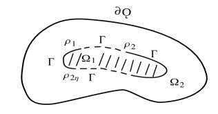
Figure 1: Geometry of the waveguide cross section of the first type. $\Gamma_{0}={\Gamma}^{\prime}\cup\partial Q$. $\Gamma\cup{\Gamma}^{\prime}\mathop{\cup}\limits_{i}\rho_{i}={\rm l}$ $\left({{\Gamma}^{\prime}\cap\Gamma=\emptyset}\right)$, $\Omega=\Omega_{1}\cup\Omega_{2}\cup\Gamma$.

Let $\rho_{i}\in{\rm l}$ be arbitrary $2N$ points $\rho_{i}\neq\rho_{j}$ dividing ${\rm l}$ into parts $\Gamma$ and $\Gamma^{\prime}$ such that $\Gamma={\rm l}\backslash\overline{\Gamma^{\prime}}$, $\Gamma^{\prime}={\rm l}\backslash\overline{\Gamma}$, $\Gamma\cup\Gamma^{\prime}\mathop{\cup}\limits_{i}\rho_{i}={\rm l}$ ($\Gamma\cap\Gamma^{\prime}=\emptyset)$. If $N=0$ then $\Gamma={\rm l}$, $\Gamma^{\prime}=\emptyset$. We will also use the notation $\Omega=\Omega_{1}\cup\Omega_{2}\cup\Gamma$ and $\Gamma_{0}=\partial Q\cup\Gamma^{\prime}$.

In the general case boundary $\partial\Omega$ of domain $\Omega$ contains the points with inner angles $0<\alpha\leq 2\pi$. If $\alpha=2\pi$, such a point is called edge. Domain $\Omega$ satisfies the cone property which allows us to apply the embedding and trace theorems in Sobolev spaces [1, 37].

Figure 2: Geometry of the waveguide cross section of the second type.

We will consider the problem on normal waves in a cylindrical shielded waveguide whose transversal (with respect to $Ox_{3})$ cross-section is formed by domain $Q$. We will assume also that waveguide’s filling contains two isotropic media with relative permittivity $\varepsilon_{j}$ in domain $\Omega_{j}$; $\varepsilon_{j}\geq 1$, $Im\,\varepsilon_{j}=0$, and $\mu_{j}=1$ ($j=1,2)$. Here $\Gamma_{0}$ is the projection of the surface of the infinitely thin and perfectly conducting shields and $\Gamma$ is the projection of the dielectric surfaces.

This family of waveguides contains in particular all types of shielded transmission lines: cylindrical and rectangular waveguides with partial filling, slot lines and strip lines with several slots or strips placed on a curved interface etc. [54].

Propagation of electromagnetic waves in a guiding system is described by the homogeneous system of Maxwell equations with dependence $e^{i\gamma x_{3}}$ on longitudinal coordinate $x_{3}$ [14]:

$$\begin{array}[]{l}rot\,{\rm{\bf E}}=-i{\rm{\bf H}},\;X=\left({x_{1},\;x_{2},\;x_{3}}\right)\in\Sigma,\\ rot\,{\rm{\bf H}}=i\varepsilon{\rm{\bf E}},\;x=\left({x_{1},\;x_{2}}\right),\\ {\rm{\bf E}}\left(X\right)=\left({E_{1}\left(x\right){\rm{\bf e}}_{1}+E_{2}\left(x\right){\rm{\bf e}}_{2}+E_{3}\left(x\right){\rm{\bf e}}_{3}}\right)e^{i\gamma x_{3}},\\ {\rm{\bf H}}\left(X\right)=\left({H_{1}\left(x\right){\rm{\bf e}}_{1}+H_{2}\left(x\right){\rm{\bf e}}_{2}+H_{3}\left(x\right){\rm{\bf e}}_{3}}\right)e^{i\gamma x_{3}},\\ \end{array}$$ (1)

with the boundary conditions for the tangential electric field components on the perfectly conducting surfaces

$$\left.{{\rm{\bf E}}_{t}}\right|_{M}=0,$$ (2)

the transmission conditions for the tangential electric and magnetic field components on the interface (surfaces where the permittivity is discontinuous)

$$\left[{{\rm{\bf E}}_{t}}\right]_{L}=0,\qquad\left[{{\rm{\bf H}}_{t}}\right]_{L}=0,$$ (3)

and the condition that provides finiteness of energy

$$\int\limits_{V}{\left({\varepsilon\left|{\rm{\bf E}}\right|^{2}+\left|{\rm{\bf H}}\right|^{2}}\right)dX}<\infty.$$ (4)

Here $M=\left\{{X:x\in\Gamma_{0}}\right\}$ is the shielded part of the boundary, $L=\left\{{X:\,x\in\Gamma}\right\}$ is the boundary where the permittivity undergoes breaks, and $V\subset\Sigma=\left\{{X:x\in\Omega}\right\}$ is an arbitrary bounded domain. System of Maxwell equations (1) is written in the normalized form and we use the following dimensionless variables and parameters [53, 20]: $k_{0}x\to x$, $\sqrt{\mu_{0}/\varepsilon_{0}}{\rm{\bf H}}\to{\rm{\bf H}}$, ${\rm{\bf E}}\to{\rm{\bf E}}$; $k_{0}^{2}=\varepsilon_{0}\mu_{0}\omega^{2}$, where $\varepsilon_{0}$ and $\mu_{0}$ are permittivity and permeability of vacuum (the time factor $e^{i\omega t}$ is omitted).

The problem on normal waves is an eigenvalue problem for the system of Maxwell equations with respect to spectral parameter $\gamma$. Eigenfunctions corresponding to certain complex values of a longitudinal wave number $\gamma$ are usually called the normal waves of the waveguide.

Write system of Maxwell equations (1) in the form

$$\frac{\partial H_{3}}{\partial x_{2}}-i\gamma H_{2}=i\varepsilon E_{1},\quad\frac{\partial E_{3}}{\partial x_{2}}-i\gamma E_{2}=-iH_{1},\quad i\gamma H_{1}-\frac{\partial H_{3}}{\partial x_{1}}=i\varepsilon E_{2},$$

$$i\gamma E_{1}-\frac{\partial E_{3}}{\partial x_{1}}=-iH_{2},\quad\frac{\partial H_{2}}{\partial x_{1}}-\frac{\partial H_{1}}{\partial x_{2}}=i\varepsilon E_{3},\quad\frac{\partial E_{2}}{\partial x_{1}}-\frac{\partial E_{1}}{\partial x_{2}}=-iH_{3},$$

and express functions $E_{1}$, $H_{1}$, $E_{2}$, and $H_{2}$ via $E_{3}$ and $H_{3}$ from the first, second, fourth, and fifth equalities

$$E_{1}=\frac{i}{\tilde{k}^{2}}\left({\gamma\frac{\partial E_{3}}{\partial x_{1}}-\frac{\partial H_{3}}{\partial x_{2}}}\right),\quad E_{2}=\frac{i}{\tilde{k}^{2}}\left({\gamma\frac{\partial E_{3}}{\partial x_{2}}+\frac{\partial H_{3}}{\partial x_{1}}}\right),$$ (5)

$$H_{1}=\frac{i}{\tilde{k}^{2}}\left({\varepsilon\frac{\partial E_{3}}{\partial x_{2}}+\gamma\frac{\partial H_{3}}{\partial x_{1}}}\right),\quad H_{2}=\frac{i}{\tilde{k}^{2}}\left({-\varepsilon\frac{\partial E_{3}}{\partial x_{1}}+\gamma\frac{\partial H_{3}}{\partial x_{2}}}\right);\tilde{k}^{2}=\varepsilon-\gamma^{2}.$$

Note that this representation is possible if $\gamma^{2}\neq\varepsilon_{1}$ and $\gamma^{2}\neq\varepsilon_{2}$.

It follows from (5) that the field of a normal wave can be expressed via two scalar functions

$$\Pi\left({x_{1},x_{2}}\right)=E_{3}\left({x_{1},x_{2}}\right),\quad\Psi\left({x_{1},x_{2}}\right)=H_{3}\left({x_{1},x_{2}}\right).$$

Thus the problem on normal waves is reduced to a boundary eigenvalue problem for functions $\Pi$ and $\Psi$. Let us write down this problem. From (1) and (2) we have the following eigenvalue problem: to find $\gamma\in C$ called eigenvalues such that there exist nontrivial solutions of the Helmholtz equations

$$\Delta\Pi+\tilde{k}^{2}\Pi=0,\quad x=\left({x_{1},x_{2}}\right)\in\Omega_{1}\cup\Omega_{2},$$

$$\Delta\Psi+\tilde{k}^{2}\Psi=0,\quad\tilde{k}^{2}=\tilde{k}_{j}^{2}=\varepsilon_{j}-\gamma^{2},$$ (6)

satisfying the boundary conditions on $\Gamma_{0}$

$$\left.\Pi\right|_{\Gamma_{0}}=0,\quad\left.{\frac{\partial\Psi}{\partial n}}\right|_{\Gamma_{0}}=0,$$ (7)

the transmission conditions on $\Gamma$

$$\left[\Pi\right]_{\Gamma}=0,\,\,\left[\Psi\right]_{\Gamma}=0,\quad\gamma\left[{\frac{1}{\tilde{k}^{2}}\frac{\partial\Psi}{\partial\tau}}\right]_{\Gamma}+\left[{\frac{\varepsilon}{\tilde{k}^{2}}\frac{\partial\Pi}{\partial n}}\right]_{\Gamma}=0,\,\,\gamma\left[{\frac{1}{\tilde{k}^{2}}\frac{\partial\Pi}{\partial\tau}}\right]_{\Gamma}-\left[{\frac{1}{\tilde{k}^{2}}\frac{\partial\Psi}{\partial n}}\right]_{\Gamma}=0,$$ (8)

and the energy (‘edge’) condition

$$\int\limits_{\Omega}{(\left|{\nabla\Pi}\right|^{2}+\left|{\nabla\Psi}\right|^{2}+\left|\Pi\right|^{2}+\left|\Psi\right|^{2})dx}<\infty.$$ (9)

Here $n$ and $\tau$ denote the (exterior to $\Omega_{2}$) normal and tangential unit vectors such that $x_{1}\times x_{2}=\tau\times n$. Square brackets $\left[f\right]_{\Gamma}=\left.{f_{2}}\right|_{\Gamma}-\left.{f_{1}}\right|_{\Gamma}$ denote the difference of limiting values of a function on $\Gamma$ in domains $\Omega_{2}$ and $\Omega_{1}$. Conditions (7) are to be satisfied on both sides of the part of boundary $\Gamma^{\prime}$.

In order to obtain (6)–(9) we used formulas (5). Conditions (7)–(9) are another form of conditions (2)–(4). Thus the longitudinal components of a normal wave satisfy (6)–(9). The inverse assertion is true. If $\Pi$ and $\Psi$ is a solution of problem (6)–(9) then the transversal components can be determined by (5). The field $E$, $H$ will satisfy all conditions (1) and (2)–(4). The equivalence of the reduction to problem (6)–(9) is not valid only for $\gamma^{2}=\varepsilon_{1}$ or $\gamma^{2}=\varepsilon_{2}$; in this case it is necessary to study system (1) directly.

System of equations (6) with boundary conditions (7), transmission conditions (8), and condition (9) constitutes a boundary eigenvalue problem that will be a subject of our study. Note that coefficient $\varepsilon$ is not continuous and the transmission conditions contain spectral parameter $\gamma$. Moreover, boundary $\Gamma$ may have ‘edges’.

Let us formulate a definition of the solution to problem (6)–(9) that will be used in the further analysis.

We will look for solutions to problem (6)–(9) in the Sobolev spaces [1, 37]

$$H_{0}^{1}\left(\Omega\right)=\left\{{f:f\in H^{1}\left(\Omega\right),\,\,\,\left.f\right|_{\Gamma_{0}}=0}\right\},\quad\mathord{\buildrel\lower 3.0pt\hbox{$\scriptscriptstyle\frown$}\over{H}}^{1}\left(\Omega\right)=\left\{{f:f\in H^{1}\left(\Omega\right),\,\,\,\int\limits_{\Omega}{fdx}=0}\right\}$$

with the inner product and the norm

$$\left({f,g}\right)_{1}=\int\limits_{\Omega}{\nabla f\nabla\bar{g}dx},\quad\left\|f\right\|_{1}^{2}=\left({f,f}\right)_{1}.$$

The seminorm $\left\|{\,\cdot\,}\right\|_{1}$ in $H^{1}\left(\Omega\right)$ is a norm in $H_{0}^{1}\left(\Omega\right)$ and $\mathord{\buildrel\lower 3.0pt\hbox{$\scriptscriptstyle\frown$}\over{H}}^{1}\left(\Omega\right)$ because sesquilinear form $\left({f,g}\right)_{1}$ in these spaces is coercive [1]. Note that it is sufficient to use the boundedness of $\Omega$ in order to prove that the form is coercive in $H_{0}^{1}\left(\Omega\right)$; however it is necessary to use the cone property for the proof of the coercive property of the form in $\mathord{\buildrel\lower 3.0pt\hbox{$\scriptscriptstyle\frown$}\over{H}}^{1}\left(\Omega\right))$. Spaces $H_{0}^{1}\left(\Omega\right)$ and $\mathord{\buildrel\lower 3.0pt\hbox{$\scriptscriptstyle\frown$}\over{H}}^{1}\left(\Omega\right)$ can be defined as a supplement of spaces of infinitely smooth functions $C_{0}^{\infty}\left(\Omega\right)$ and $C^{\infty}\left(\Omega\right)$ with respect to the norm $\left\|{\,\cdot\,}\right\|_{1}$ (under the condition $\left\|f\right\|_{1}<\infty)$; $\mathord{\buildrel\lower 3.0pt\hbox{$\scriptscriptstyle\frown$}\over{H}}^{1}\left(\Omega\right)$ is a subspace of functions from $H^{1}\left(\Omega\right)$ which are orthogonal to the unit function.

Under the above assumptions the domain $\Omega$ satisfies cone property: there is a cone

$$K_{0}=\left\{{x:0\leq x_{1}\leq b,\,\,x_{2}^{2}\leq ax_{1}^{2};\,\,a>0,\,\,b>0}\right\}$$

such that any point $P\in\Omega$ can be a vertex of cone $K_{p}$ which is equal to $K_{0}$, and the cone belongs to $\Omega$, $K_{p}\subset\Omega$. This property allows us to apply the Sobolev trace theorem [1] and consider the trace of function $f\in H^{1}\left(\Omega\right)$ on $\Gamma$ as an element of space $H^{1/2}\left(\Gamma\right)$. Due to the trace theorem, the relation $\left.f\right|_{\Gamma_{0}}=0$ means that the function is equal to zero in $H^{1/2}\left({\Gamma_{0}}\right)$. For any function $f\in H^{1}\left(\Omega\right)$ we have $\left[f\right]_{\Gamma}=0$ in the sense of space $H^{1/2}\left(\Gamma\right)$; and vice versa, if $\left[f\right]_{\Gamma}=0$, $\left.f\right|_{\Omega_{1}}\in H^{1}\left({\Omega_{1}}\right)$, $\left.f\right|_{\Omega_{2}}\in H^{1}\left({\Omega_{2}}\right)$, then $f\in H^{1}\left(\Omega\right)$. On the part of the boundary $\Gamma^{\prime}\subset\Gamma_{0}$ the trace theorem should be applied on both sides of $\Gamma^{\prime}$; in this case functions $f\in H^{1}\left(\Omega\right)$ have in general different traces on different sides of $\Gamma^{\prime}$. Note also that the following embeddings

$$H_{0}^{1}\left(\Omega\right)\subset H_{0}^{1}\left(Q\right)\subset H^{1}\left(Q\right)\subset H^{1}\left(\Omega\right),$$

hold but all embeddings are not dense if $\Gamma^{\prime}\neq\emptyset$.

Assume that $\Pi\in H_{0}^{1}\left(\Omega\right)$, $\Psi\in\mathord{\buildrel\lower 3.0pt\hbox{$\scriptscriptstyle\frown$}\over{H}}^{1}\left(\Omega\right)$. Condition (6) is fulfilled in $\Omega_{1}$ and $\Omega_{2}$ in terms of distributions [31]. Moreover, we have for the boundary condition on $\Gamma_{0}$

$$\left.{\Pi_{j}}\right|_{\Gamma_{0}\cap\partial\Omega_{j}}\in H^{1/2}\left({\Gamma_{0}\cap\partial\Omega_{j}}\right),\quad\left.{\frac{\partial\Psi_{j}}{\partial n}}\right|_{\Gamma_{0}\cap\partial\Omega_{j}}\in H^{-1/2}\left({\Gamma_{0}\cap\partial\Omega_{j}}\right).$$

For the transmission condition on $\Gamma$, we have

$$\left.\Pi\right|_{\Gamma}\in H^{1/2}\left(\Gamma\right),\quad\left.\Psi\right|_{\Gamma}\in H^{1/2}\left(\Gamma\right),$$

$$\left.{\frac{\partial\Pi_{j}}{\partial n}}\right|_{\Gamma},\,\,\left.{\frac{\partial\Psi_{j}}{\partial n}}\right|_{\Gamma}\in H^{-1/2}\left(\Gamma\right),\quad\left.{\frac{\partial\Pi}{\partial\tau}}\right|_{\Gamma},\,\,\left.{\frac{\partial\Psi}{\partial\tau}}\right|_{\Gamma}\in H^{-1/2}\left(\Gamma\right),$$

where $\Pi_{j}$ and $\Psi_{j}$ are restrictions of $\Pi$ and $\Psi$ on $\Omega_{j}$.

Let us give a variational formulation of problem (3)–(9). Multiply equations (3) and (4) by arbitrary test functions $\bar{u}\in H_{0}^{1}\left(\Omega\right)$ and $\bar{v}\in\mathord{\buildrel\lower 3.0pt\hbox{$\scriptscriptstyle\frown$}\over{H}}^{1}\left(\Omega\right)$ (we may assume that these functions are continuously differentiable in $\bar{\Omega}_{1}$ and $\bar{\Omega}_{2}$ because these spaces form dense sets in $H_{0}^{1}\left(\Omega\right)$ and $\mathord{\buildrel\lower 3.0pt\hbox{$\scriptscriptstyle\frown$}\over{H}}^{1}\left(\Omega\right))$, and apply Green’s formula [31], [4] for each domain $\Omega_{j}$ separately. Note that the possibility of applying Green’s formula for these functions is proved in [31] and [4], p. 618. We have

$$\int\limits_{\Omega_{j}}{\nabla\Pi\nabla\bar{u}dx}-\tilde{k}_{j}^{2}\int\limits_{\Omega_{j}}{\Pi\bar{u}dx}=\left({-1}\right)^{j}\int\limits_{\partial\Omega_{j}}{\left.{\frac{\partial\Pi}{\partial n}}\right|_{\partial\Omega_{j}}\bar{u}d\tau},$$ (10)

$$\int\limits_{\Omega_{j}}{\nabla\Psi\nabla\bar{v}dx}-\tilde{k}_{j}^{2}\int\limits_{\Omega_{j}}{\Psi\bar{v}dx}=\left({-1}\right)^{j}\int\limits_{\partial\Omega_{j}}{\left.{\frac{\partial\Psi}{\partial n}}\right|_{\partial\Omega_{j}}\bar{v}d\tau};\,\,\,j=1,2.$$ (11)

Then, substituting the normal derivatives from (7) and (8) to (10) and (11) we obtain the variational relation

$$\int\limits_{\Omega}{\frac{1}{\tilde{k}^{2}}\left({\varepsilon\nabla\Pi\nabla\bar{u}+\nabla\Psi\nabla\bar{v}}\right)dx}-\int\limits_{\Omega}{\left({\varepsilon\Pi\bar{u}+\Psi\bar{v}}\right)dx}-\gamma\left[{\frac{1}{\tilde{k}^{2}}}\right]\int\limits_{\Gamma}{\left({\frac{\partial\Pi}{\partial\tau}\bar{v}-\frac{\partial\Psi}{\partial\tau}\bar{u}}\right)d\tau}=0,\\$$ (12)

which is derived for smooth functions $u$, $v$. In Section 2.1 we will prove the continuity of the sesquilinear forms defined by the integrals in (12). Hence relation (12) can be extended to arbitrary functions $u\in H_{0}^{1}\left(\Omega\right)$, $v\in\mathord{\buildrel\lower 3.0pt\hbox{$\scriptscriptstyle\frown$}\over{H}}^{1}\left(\Omega\right)$. Here and below, the $f$ under the integral sign in $\int\limits_{\Gamma}{fd\tau}$ is the trace of the function on $\Gamma$.

For $v\equiv 1$, $u\equiv 0$ we obtain in a similar manner

$$\int\limits_{\Omega}{\Psi dx}=-\int\limits_{\Gamma}{\left[{\frac{1}{\tilde{k}^{2}}\frac{\partial\Psi}{\partial n}}\right]_{\Gamma}d\tau}=-\gamma\left[{\frac{1}{\tilde{k}^{2}}}\right]\int\limits_{\Gamma}{\left.{\frac{\partial\Pi}{\partial\tau}}\right|_{\Gamma}d\tau}=0;$$ (13)

consequently, the choice of space $\mathord{\buildrel\lower 3.0pt\hbox{$\scriptscriptstyle\frown$}\over{H}}^{1}\left(\Omega\right)$ does not contradict to the choice of the space of solutions to problem (6)–(9). In (13) we used the condition

$$\left.\Pi\right|_{\rm l}\in\tilde{H}^{1/2}\left(\bar{\Gamma}\right):=\{\varphi:\varphi\in H^{1/2}({\rm l}),\quad\mbox{supp}\quad\varphi\subset\bar{\Gamma}\},$$

since $\Pi\in H_{0}^{1}\left(\Omega\right)$, so that the set of functions $C_{0}^{\infty}\left(\Gamma\right)$ is dense in $\tilde{H}^{1/2}\left(\bar{\Gamma}\right)$.

Definition 1. The pair of functions

$\Pi\in H_{0}^{1}\left(\Omega\right)$, $\Psi\in\mathord{\buildrel\lower 3.0pt\hbox{$\scriptscriptstyle\frown$}\over{H}}^{1}\left(\Omega\right)$ $(\left\|\Pi\right\|_{1}+\left\|\Psi\right\|_{1}\neq 0)$

is called the eigenvector of problem (6)–(9) corresponding to eigenvalue $\gamma_{0}$ if variational relation (12) holds for $u\in H_{0}^{1}(\Omega)$, $v\in\mathord{\buildrel\lower 3.0pt\hbox{$\scriptscriptstyle\frown$}\over{H}}^{1}\left(\Omega\right)$.

Thus, if $\Pi\in H_{0}^{1}\left(\Omega\right)$ and $\Psi\in\mathord{\buildrel\lower 3.0pt\hbox{$\scriptscriptstyle\frown$}\over{H}}^{1}\left(\Omega\right)$ and (6)–(9) are fulfilled, variational relation (12) also holds. The inverse assertion is true. Choosing $u$ and $v$ with a support in $\Omega_{j}$ we have that equations (6) are fulfilled in terms of distributions. The first condition in (7), the first condition in (8), and (9) are fulfilled by the definition of spaces $H_{0}^{1}\left(\Omega\right)$ and $\mathord{\buildrel\lower 3.0pt\hbox{$\scriptscriptstyle\frown$}\over{H}}^{1}\left(\Omega\right)$. If we choose $u\equiv 0$ and assume that the support of $v$ contains the part $\Gamma_{1}$ of boundary $\Gamma_{0}$, then from (12) and Green’s formula we find [4], [31] that the second condition in (7) is also fulfilled in term of distributions. Choosing arbitrary $u$ and $v$ on $\Gamma$ in (12) and applying formulas (10) and (11) we obtain the relation

$$\int\limits_{\Gamma}{\left({\gamma\left[{\frac{1}{\tilde{k}^{2}}\frac{\partial\Psi}{\partial\tau}}\right]_{\Gamma}+\left[{\frac{\varepsilon}{\tilde{k}^{2}}\frac{\partial\Pi}{\partial n}}\right]_{\Gamma}}\right)\bar{u}d\tau}+\int\limits_{\Gamma}{\left({\gamma\left[{\frac{1}{\tilde{k}^{2}}\frac{\partial\Pi}{\partial\tau}}\right]_{\Gamma}-\left[{\frac{1}{\tilde{k}^{2}}\frac{\partial\Psi}{\partial n}}\right]_{\Gamma}}\right)\bar{v}d\tau=0},$$

which yields that the second and third condition in (8) are fulfilled in terms of distributions.

Let us give some remarks concerning the smoothness of eigenvectors of problem (6)–(9). It is well known [28, 38] that solutions $\Pi$ and $\Psi$ of homogeneous Helmholtz equations (6) are infinitely smooth in $\Omega_{1}$ and $\Omega_{2}$: $\Pi,\Psi\in C^{\infty}\left({\Omega_{1}\cup\Omega_{2}}\right)$; consequently, equations (6) are satisfied in the classical sense. In a vicinity of an arbitrary smooth part $\Gamma_{1}$ of boundary $\Gamma_{0}$ conditions (7) are also fulfilled in the classical sense and functions $\Pi$ and $\Psi$ are infinitely smooth up to the boundary. The behavior of $\Pi$ and $\Psi$ close to edge (angle) points was analyzed in [24]. Note that in what follows we will not use the smoothness of functions $\Pi$ and $\Psi$.

3 Eigenvalue problem for operator pencil

Multiplying (12) by $\tilde{k}_{1}^{2}\tilde{k}_{2}^{2}$ we rewrite it in the form

$$\begin{array}[]{l}{\begin{array}[]{*{20}c}\hfill\hfil&\hfill\hfil\\ \end{array}}\gamma^{4}\int\limits_{\Omega}{\left({\varepsilon\Pi\bar{u}+\Psi\bar{v}}\right)dx}+\gamma^{2}\left({\int\limits_{\Omega}{\left({\varepsilon\nabla\Pi\nabla\bar{u}+\nabla\Psi\nabla\bar{v}}\right)dx}-}\right.\\ \left.{-\left({\varepsilon_{1}+\varepsilon_{2}}\right)\int\limits_{\Omega}{\left({\varepsilon\Pi\bar{u}+\Psi\bar{v}}\right)dx}}\right)+\left({\varepsilon_{1}-\varepsilon_{2}}\right)\gamma\int\limits_{\Gamma}{\left({\frac{\partial\Pi}{\partial\tau}\bar{v}-\frac{\partial\Psi}{\partial\tau}\bar{u}}\right)d\tau+}\\ \;\;+\varepsilon_{1}\varepsilon_{2}\left({\int\limits_{\Omega}{\left({\varepsilon\Pi\bar{u}+\Psi\bar{v}}\right)dx}-\int\limits_{\Omega}{\left({\nabla\Pi\nabla\bar{u}+\frac{1}{\varepsilon}\nabla\Psi\nabla\bar{v}}\right)dx}}\right)=0,\\ {\begin{array}[]{*{20}c}{{\begin{array}[]{*{20}c}\hfill}{\hfil&\hfill\hfil&\hfill\hfil\\ \end{array}\hfill}}&\hfill\hfil&\hfill\hfil\\ \end{array}}\forall u\in H_{0}^{1}\left(\Omega\right),\,\,v\in\mathord{\buildrel\lower 3.0pt\hbox{$\scriptscriptstyle\frown$}\over{H}}^{1}\left(\Omega\right).\\ \end{array}$$ (14)

Let $H=H_{0}^{1}\left(\Omega\right)\times\mathord{\buildrel\lower 3.0pt\hbox{$\scriptscriptstyle\frown$}\over{H}}^{1}\left(\Omega\right)$ be the Cartesian product of the Hilbert spaces with the inner product and the norm

$$\left({f,g}\right)=\left({f_{1},g_{1}}\right)_{1}+\left({f_{2},g_{2}}\right)_{1},\quad\left\|f\right\|^{2}=\left\|{f_{1}}\right\|_{1}^{2}+\left\|{f_{2}}\right\|_{1}^{2},$$

where

$$f,g\in H,\quad f=\left({f_{1},f_{2}}\right)^{\rm T},\quad g=\left({g_{1},g_{2}}\right)^{\rm T},\quad f_{1},g_{1}\in H_{0}^{1}\left(\Omega\right),\quad f_{2},g_{2}\in\mathord{\buildrel\lower 3.0pt\hbox{$\scriptscriptstyle\frown$}\over{H}}^{1}\left(\Omega\right).$$

Then the integrals in (14) can be considered as sesquilinear forms on ${\bf C}$ defined in $H$ with respect to vector-functions such that

$$f_{1}=\Pi,\quad f_{2}=\Psi,\quad g_{1}=u,\quad g_{2}=v.$$

These forms (if they are bounded) define, in accordance with the results of [21], linear bounded operators $T:\,H\to H$

$$t\left({f,g}\right)=\left({Tf,g}\right),\quad\forall g\in H.$$ (15)

Linearity follows here from the linearity of the form with respect to the first argument and continuity from the estimates

$$\left\|{Tf}\right\|^{2}=t\left({f,Tf}\right)\leq C\left\|f\right\|\,\left\|{Tf}\right\|.$$

Consider the following quadratic forms and corresponding operators

$$a_{1}\left({f,g}\right):=\int\limits_{\Omega}{\left({\varepsilon\nabla f_{1}\nabla\bar{g}_{1}+\nabla f_{2}\nabla\bar{g}_{2}}\right)dx}=\left({A_{1}f,g}\right),\quad\forall g\in H,$$

$$a_{2}\left({f,g}\right):=\int\limits_{\Omega}{\left({\nabla f_{1}\nabla\bar{g}_{1}+\frac{1}{\varepsilon}\nabla f_{2}\nabla\bar{g}_{2}}\right)dx}=\left({A_{2}f,g}\right),\quad\forall g\in H,$$

$$k\left({f,g}\right):=\int\limits_{\Omega}{\left({\varepsilon f_{1}\bar{g}_{1}+f_{2}\bar{g}_{2}}\right)dx}=\left({Kf,g}\right),\quad\forall g\in H,$$

$$s\left({f,g}\right):=\int\limits_{\Gamma}{\left({\frac{\partial f_{1}}{\partial\tau}\bar{g}_{2}-\frac{\partial f_{2}}{\partial\tau}\bar{g}_{1}}\right)d\tau}=\left({Sf,g}\right),\forall g\in H.$$ (16)

It is easy to see that forms $a_{1}\left({f,g}\right)$ and $a_{2}\left({f,g}\right)$ are bounded. The same property for the form $k\left({f,g}\right)$ follows from Poincare’s inequality [1].

Let us prove that form $s\left({f,g}\right)$ is also bounded. Assume that functions $f_{1},\,f_{2},\,g_{1},\,g_{2}\in C^{1}\left({\bar{\Omega}_{1}}\right)\cap C^{1}\left({\bar{\Omega}_{2}}\right)$. Then

$$\int\limits_{\Gamma}{\left({\frac{\partial f_{1}}{\partial\tau}\bar{g}_{2}-\frac{\partial f_{2}}{\partial\tau}\bar{g}_{1}}\right)d\tau}=\int\limits_{\Omega}{\frac{\xi}{2}\left({\frac{\partial f_{1}}{\partial x_{2}}\frac{\partial\bar{g}_{2}}{\partial x_{1}}-\frac{\partial f_{1}}{\partial x_{1}}\frac{\partial\bar{g}_{2}}{\partial x_{2}}+\frac{\partial f_{2}}{\partial x_{1}}\frac{\partial\bar{g}_{1}}{\partial x_{2}}-\frac{\partial f_{2}}{\partial x_{2}}\frac{\partial\bar{g}_{1}}{\partial x_{1}}}\right)dx},$$

where

$$\xi=\left\{{\begin{array}[]{l}1,\,\,x\in\Omega_{1}\\ -1,\,\,x\in\Omega_{2}\\ \end{array}}\right..$$

Using the Schwartz inequality we finally obtain

$$\left|{s\left({f,g}\right)}\right|\leq\frac{1}{2}\left\|f\right\|\,\left\|g\right\|.$$ (17)

The required property of the form may be easily obtained if to extend the estimate given by (17) for arbitrary functions $f,\,g\in H$ using the continuity.

Remark. In the expression

$$\int\limits_{\Gamma}{\left({\frac{\partial f_{1}}{\partial\tau}\bar{g}_{2}-\frac{\partial f_{2}}{\partial\tau}\bar{g}_{1}}\right)d\tau}$$

$g_{1}$, $g_{2}$, $\frac{\partial f_{1}}{\partial\tau}$, and $\frac{\partial f_{2}}{\partial\tau}$ mean the restriction of elements

$$\left.{g_{1},g_{2}}\right|_{\partial\Omega_{j}}\in H^{1/2}\left({\partial\Omega_{j}}\right),\quad\frac{\partial f_{1}}{\partial\tau},\quad\left.{\frac{\partial f_{2}}{\partial\tau}}\right|_{\partial\Omega_{j}}\in H^{-1/2}\left({\partial\Omega_{j}}\right)$$

on $\Gamma$ [31]. Since on ${\rm l}$

$$\left.{f_{1}}\right|_{\Gamma^{\prime}}=0,\quad\left.{g_{1}}\right|_{\Gamma^{\prime}}=0,\quad\mbox{supp}\;f_{1}\subset\bar{\Gamma},\quad\mbox{supp}\;g_{1}\subset\bar{\Gamma},$$

the following formulas of the integration by parts hold

$$\int\limits_{\Gamma}{\frac{\partial f_{1}}{\partial\tau}\bar{g}_{2}d\tau}=-\int\limits_{\Gamma}{\frac{\partial\bar{g}_{2}}{\partial\tau}f_{1}d\tau},\;\;\int\limits_{\Gamma}{\frac{\partial f_{2}}{\partial\tau}\bar{g}_{1}d\tau}=-\int\limits_{\Gamma}{\frac{\partial\bar{g}_{1}}{\partial\tau}f_{2}d\tau}.$$ (18)

Now the variational problem given by (14) can be written in the operator form

$$\left({L\left(\gamma\right)f,g}\right)=0,\quad\forall g\in H,$$

which is equivalent to the following equation for the operator-valued pencil

$$\begin{array}[]{l}{\begin{array}[]{*{20}c}{{\begin{array}[]{*{20}c}\hfill}{\hfil&\hfill\hfil&\hfill\hfil\\ \end{array}\hfill}}&\hfill\hfil&\hfill\hfil\\ \end{array}}L\left(\gamma\right)f=0,\,\,L\left(\gamma\right):H\to H,\\ L\left(\gamma\right):=\gamma^{4}K+\gamma^{2}\left({A_{1}-\left({\varepsilon_{1}+\varepsilon_{2}}\right)K}\right)+\left({\varepsilon_{1}-\varepsilon_{2}}\right)\gamma S+\varepsilon_{1}\varepsilon_{2}\left({K-A_{2}}\right),\\ \end{array}$$ (19)

where all the operators are bounded.

Equation (19) is another form of variational relation (14). Eigenvalues and eigenvectors of the pencil coincide with eigenvalues and eigenfunctions of problem (6)–(9) for $\gamma^{2}\neq\varepsilon_{1}$, $\gamma^{2}\neq\varepsilon_{2}$ according to the definition.

Thus the problem on normal waves is reduced to an eigenvalue problem for pencil $L\left(\gamma\right)$.

Now we consider the properties of the operators in (16).

Lemma 1. The operators $A_{1}$ and $A_{2}$ are uniformly positive:

$$I\leq A_{1}\leq\varepsilon_{\max}I,\quad\varepsilon_{\max}^{-1}I\leq A_{2}\leq I,$$ (20)

where $\varepsilon_{\max}=\max\left({\varepsilon_{1},\varepsilon_{2}}\right)$ and $I$ is the unit operator in $H$.

The proof of the lemma is reduced to the verification of simple inequalities

$$\left\|f\right\|^{2}\leq\left({A_{1}f,f}\right)\leq\varepsilon_{\max}\left\|f\right\|^{2},\qquad\varepsilon_{\max}^{-1}\left\|f\right\|^{2}\leq\left({A_{2}f,f}\right)\leq\left\|f\right\|^{2}.$$

Lemma 2. The operator $S$ is selfadjoint, $S=S^{\ast}$, and the following inequalities hold

$$-\frac{1}{2}I\leq S\leq\frac{1}{2}I.$$ (21)

The selfadjointness of operator $S$ follows from the equality

$$\int\limits_{\Gamma}{\left({\frac{\partial f_{1}}{\partial\tau}\bar{g}_{2}-\frac{\partial f_{2}}{\partial\tau}\bar{g}_{1}}\right)d\tau}=\int\limits_{\Gamma}{\left({\frac{\partial\bar{g}_{1}}{\partial\tau}f_{2}-\frac{\partial\bar{g}_{2}}{\partial\tau}f_{1}}\right)d\tau},$$

which follows in its turn from the remark above and formulas (18). Inequalities (21) follow from (17).

Lemma 3. Operator $K$ is positive, $K>0$, and compact. The following estimate holds for its eigenvalues

$$\lambda_{n}\left(K\right)=O\left({n^{-1}}\right),\,\,\,n\to\infty.$$ (22)

It is easy to see that $\left({Kf,f}\right)>0$ for $f\neq 0$ since $\int\limits_{\Omega}{\left({\varepsilon\left|{f_{1}}\right|^{2}+\left|{f_{2}}\right|^{2}}\right)dx}=0$ is fulfilled only for $f_{1}=0$ and $f_{2}=0$ (in $H^{1}\left(\Omega\right))$.

The compactness of the operator $K$ follows from formula (22).

The proof of formula (22) is based on the Courant variational principle. From the inequality

$$\int\limits_{\Omega}{\left({\varepsilon\left|{f_{1}}\right|^{2}+\left|{f_{2}}\right|^{2}}\right)dx}\leq\varepsilon_{\max}\int\limits_{\Omega}{\left({\left|{f_{1}}\right|^{2}+\left|{f_{2}}\right|^{2}}\right)dx}$$

we obtain [8] that

$$\lambda_{n}\left(K\right)\leq\varepsilon_{\max}\lambda_{n}\left({K_{H}}\right),\quad n\geq 1,$$

where $\lambda_{n}\left({K_{H}}\right)$ are eigenvalues of the operator specified by the sesquilinear form

$$q\left({f,g}\right):=\int\limits_{\Omega}{\left({f_{1}\overline{g}_{1}+f_{2}\overline{g}_{2}}\right)dx}=\left({K_{H}f,g}\right),\quad\forall g\in H.$$ (23)

Thus it is sufficient to consider operator $K_{H}$. Formula (22) follows from the asymptotic behavior of $s$-numbers [8] of operator $K_{H}$ which can be found in [50] (Theorem 4.10.1). The statement is proved. (The proof in detail one can find in [46])

Thus all operators $A_{1}$, $A_{2}$, $K$, and $S$ are selfadjoint, and $\mbox{Ker}K=\left\{0\right\}$. There exist bounded inverse operators $A_{j}^{-1}:H\to H$ and $A_{j}^{1/2},\,\,A_{j}^{-1/2}:H\to H$; these operators are uniformly positive. Note that in this case the condition $B>0$ leads to $B=B^{\ast}$ since Hilbert space $H$ is considered on complex-valued functions. Using these lemmas we obtain

Corollary 1. Operator pencil $L\left(\gamma\right)$ is self-adjoint:

$$L^{\ast}\left(\gamma\right)=L\left(\bar{\gamma}\right).$$ (24)

From variational relation (14) we obtain

Corollary 2. Let $P$ be an operator such that

$$P\left({f_{1},f_{2}}\right)^{\rm T}=\left({-f_{1},f_{2}}\right)^{\rm T}.$$

Then

$$A_{1}=PA_{1}P,\quad A_{2}=PA_{2}P,\quad K=PKP,\quad S=-PSP,$$

and the following representation holds

$$L\left({-\gamma}\right)=PL\left(\gamma\right)P.$$ (25)

The proof of this statement follows directly from the explicit form of variational relation (14).

Note that operator $S$ does not possess the Fredholm property because $\dim\mbox{Ker}\,S=\infty$. Indeed, all functions $f=\left({f_{1},f_{2}}\right)^{\rm T}$ satisfying the additional conditions $\left.{f_{1}}\right|_{\Gamma}=0$, $\left.{f_{2}}\right|_{\Gamma}=0$ belong to the kernel of operator $S$.

4 Properties of the spectrum of pencil $L\left(\gamma\right)$

We will denote by ${\cal R}\left(L\right)$ the resolvent set of $L\left(\gamma\right)$ (consisting of all complex values of $\gamma$ at which there exists a bounded inverse operator $L^{-1}\left(\gamma\right))$ and by $\sigma\left(L\right)={\bf C}\backslash{\cal R}\left(L\right)$ the spectrum of $L\left(\gamma\right)$.

In what follows we will use the definitions of finite-meromorphic OVFs and canonical system of eigenvectors and associated vectors of an OVF formulated in [8, 10, 23]. We will consider OVFs that have eigenvalues with finite algebraic multiplicity.

Let us study the spectrum of pencil $L\left(\gamma\right)$. It is more convenient to consider a regularized pencil

$$\begin{array}[]{c}\tilde{L}\left(\gamma\right):=A_{1}^{-1/2}L\left(\gamma\right)A_{1}^{-1/2}=\gamma^{4}\tilde{K}+\gamma^{2}\left({I-\left({\varepsilon_{1}+\varepsilon_{2}}\right)\tilde{K}}\right)+\\ +\left({\varepsilon_{1}-\varepsilon_{2}}\right)\gamma\tilde{S}+\varepsilon_{1}\varepsilon_{2}\left({\tilde{K}-\tilde{A}_{2}}\right)\\ \end{array},$$ (26)

where $\tilde{K}=A_{1}^{-1/2}KA_{1}^{-1/2}$, $\tilde{S}=A_{1}^{-1/2}SA_{1}^{-1/2}$, and $\tilde{A}_{2}=A_{1}^{-1/2}A_{2}A_{1}^{-1/2}$.

It is easy to see that $\sigma\left(L\right)=\sigma\left(\tilde{L}\right)$ and the following relations hold for eigenvectors and associated vectors

$$\varphi_{j}\left(L\right)=A_{1}^{-1/2}\varphi_{j}\left(\tilde{L}\right).$$ (27)

Operators $\tilde{K}$, $\tilde{S}$ and $\tilde{A}_{2}$ keep all properties of operators $K$, $S$, and $A_{2}$ given in Lemmas 1–3 with the estimates

$$-\frac{1}{2}I\leq\tilde{S}\leq\frac{1}{2}I,\quad\varepsilon_{\max}^{-2}I\leq\tilde{A}_{2}\leq I.$$ (28)

Properties of the spectrum of pencil $L\left(\gamma\right)$ are summarized in the following theorems.

Theorem 1.

$$\sigma\left(L\right)\subset\Pi_{l}=\left\{{\gamma:\left|{Re\gamma}\right|<l}\right\}$$

i.e. for a certain $l>0$ the spectrum of pencil $L\left(\gamma\right)$ lies in the strip $\Pi_{l}$.

Proof. In order to prove this theorem, assume that $l>\sqrt{\varepsilon_{1}+\varepsilon_{2}}$ and consider the operator-valued function

$$F\left(\gamma\right):=\left({\gamma^{2}-\left({\varepsilon_{1}+\varepsilon_{2}}\right)}\right)^{-1}\tilde{L}\left(\gamma\right)=\gamma^{2}\tilde{K}+I+\gamma^{-1}T\left(\gamma\right),$$ (29)

in the domain $D_{0}=\left\{{\gamma:\left|\gamma\right|>l}\right\}$, where

$$T\left(\gamma\right)=\gamma\left({\gamma^{2}-\left({\varepsilon_{1}+\varepsilon_{2}}\right)}\right)^{-1}\times\left({\left({\varepsilon_{1}+\varepsilon_{2}}\right)I+\left({\varepsilon_{1}-\varepsilon_{2}}\right)\gamma\tilde{S}+\varepsilon_{1}\varepsilon_{2}\left({\tilde{K}-\tilde{A}_{2}}\right)}\right)$$

is a holomorphic and bounded operator-valued function in the domain $D_{0}$: $\left\|{T\left(\gamma\right)}\right\|\leq T_{0}$ for $\gamma\in D_{0}$. One can see that $\sigma\left(\tilde{L}\right)\cap D_{0}=\sigma\left(F\right)\cap D_{0}$. If $\left|{Re\gamma}\right|>l$, there exists a bounded operator

$$R\left(\gamma\right)=\left({\gamma^{2}\tilde{K}+I}\right)^{-1}$$

and its norm can be calculated by the formula (see [9], p. 309)

$$\|R(\gamma)\|=\frac{\gamma^{-2}}{d(-\gamma^{-2})},$$

where $d(\mu)$ is the distance from point $\mu$ to spectrum of operator $\tilde{K}$. Thus we obtain the estimates

$$\left\|{R\left(\gamma\right)}\right\|\leq\frac{\left|{\gamma^{-2}}\right|}{\left|{Im\gamma^{-2}}\right|}=\frac{\left|\gamma\right|^{2}}{2\left|{\gamma}^{\prime}\right|\left|{\gamma}^{\prime\prime}\right|}=\frac{1}{2}\left({\frac{\left|{\gamma}^{\prime}\right|}{\left|{\gamma}^{\prime\prime}\right|}+\frac{\left|{\gamma}^{\prime\prime}\right|}{\left|{\gamma}^{\prime}\right|}}\right)\leq\frac{1}{2}\left({1+\frac{\left|\gamma\right|}{l}}\right)$$

when $\left|{\gamma}^{\prime\prime}\right|>\left|{\gamma}^{\prime}\right|$ and $\left\|{R\left(\gamma\right)}\right\|=1$ for $\left|{\gamma}^{\prime\prime}\right|\leq\left|{\gamma}^{\prime}\right|$ where $\gamma={\gamma}^{\prime}+i{\gamma}^{\prime\prime}$. Choosing the value $l>T_{0}$ we obtain

$$\left\|{\gamma^{-1}T\left(\gamma\right)R\left(\gamma\right)}\right\|\leq\frac{1}{2}\left({1+\frac{\left|\gamma\right|}{l}}\right)\frac{T_{0}}{\left|\gamma\right|}<1.$$

Hence, there exists a bounded operator

$$F^{-1}\left(\gamma\right)=R\left(\gamma\right)\left({I+\gamma^{-1}T\left(\gamma\right)R\left(\gamma\right)}\right)^{-1},$$

which yields the existence of bounded operators $\tilde{L}^{-1}\left(\gamma\right)$ and $L^{-1}\left(\gamma\right)$ for $\gamma\in\Pi_{l}=\left\{{\gamma:\left|{Re\gamma}\right|<l}\right\}$ outside the strip $\Pi_{l}$.

Corollary 3. The resolvent set of pencil $L\left(\gamma\right)$ is not empty,

$${\bf C}\backslash\Pi_{l}\subset{\cal R}\left(L\right).$$

Theorem 2. The spectrum of pencil $L\left(\gamma\right)$ is symmetric with respect to the real and imaginary axes:

$$\sigma\left(L\right)=\overline{\sigma\left(L\right)}=-\sigma\left(L\right).$$

If $\gamma_{0}$ is an eigenvalue of pencil $L\left(\gamma\right)$ corresponding to the eigenvector $\left({\Pi,\Psi}\right)^{\rm T}$ then $-\gamma_{0},\bar{\gamma}_{0}$, and $-\bar{\gamma}_{0}$ are also eigenvalues of pencil $L\left(\gamma\right)$ corresponding to the eigenvectors $\left({-\Pi,\Psi}\right)^{\rm T},$ $\left({\bar{\Pi},\bar{\Psi}}\right)^{\rm T}$, and $\left({-\bar{\Pi},\bar{\Psi}}\right)^{\rm T}$ with the same multiplicity.

Proof. The first assertion of Theorem 4 follows from (24) and (25). Proof of the second assertion is actually a simple verification of variational relation (14). Note that associated vectors at $\bar{\gamma}_{0}$ can be obtained by taking complex conjugation of associated vectors corresponding to $\gamma_{0}$.

Theorem 3. Set $\delta=\left({\varepsilon_{2}-\varepsilon_{1}}\right)/2,$

$$I_{0}=\left\{{\gamma:Im\gamma=0,\frac{\left({\delta^{2}+4\varepsilon_{1}}\right)^{1/2}-\left|\delta\right|}{2}\leq\left|\gamma\right|\leq\frac{\left({\delta^{2}+4\varepsilon_{2}}\right)^{1/2}+\left|\delta\right|}{2}}\right\}.$$

In the domain ${\bf C}\backslash I_{0}$ the spectrum of pencil $\sigma\left(L\right)$ is a set of isolated eigenvalues with finite algebraic multiplicity. The points $\gamma_{j}=\pm\sqrt{\varepsilon_{i}}$ ($i=1,2$) are the degeneration values of pencil $L\left(\gamma\right):\dim\ker L\left({\gamma_{j}}\right)=\infty.$

Proof. Taking $\gamma=\gamma^{\prime}+i\gamma^{\prime\prime}$ with $\gamma^{\prime\prime}\neq 0$ we have

$$Im\left[{\frac{1}{\gamma^{\prime\prime}}\left({\gamma A_{1}-2\delta S-\frac{\varepsilon_{1}\varepsilon_{2}}{\gamma}A_{2}}\right)}\right]=A_{1}+\frac{\varepsilon_{1}\varepsilon_{2}}{\left|\gamma\right|^{2}}A_{2}\geq I;$$

hence, in line with [9], the operator

$$L_{0}\left(\gamma\right):=\gamma^{2}A_{1}-2\gamma\delta S-\varepsilon_{1}\varepsilon_{2}A_{2}$$

has a bounded inverse and $L\left(\gamma\right)$ is a Fredholm pencil with $\mbox{ind }L\left(\gamma\right)=0$.

Introduce the operator $A^{\prime}_{1}:\,H\to H$ defined by the form ($\xi$ was defined before formula (17))

$$a^{\prime}_{1}\left({f,g}\right):=\int\limits_{\Omega}{\xi\left({\varepsilon\nabla f_{1}\nabla\bar{g}_{1}+\nabla f_{2}\nabla\bar{g}_{2}}\right)dx}=\left({A^{\prime}_{1}f,g}\right),\quad\forall g\in H,$$ (30)

and the operator

$$\tilde{A}^{\prime}_{1}=A_{1}^{-1/2}A^{\prime}_{1}A_{1}^{-1/2}.$$

For these operators the following estimates hold

$$-\varepsilon_{\max}I\leq A^{\prime}_{1}\leq\varepsilon_{\max}I,\quad-I\leq\tilde{A}^{\prime}_{1}\leq I.$$ (31)

Set $p=\left({\left({\varepsilon_{2}+\varepsilon_{1}}\right)/2}\right)^{1/2}$. For real $\gamma\notin I_{0}$ the estimate $\left|{\gamma^{2}-p^{2}}\right|>\left|\delta\right|\left({1+\left|\gamma\right|}\right)$ holds; consequently, the operator

$$\tilde{L}_{0}\left(\gamma\right):=A_{1}^{-1/2}L_{0}\left(\gamma\right)A_{1}^{-1/2}=\left({\gamma^{2}-p^{2}}\right)I-2\gamma\delta\tilde{S}+\delta\tilde{A}^{\prime}_{1}$$

has a bounded inverse as well as operator $L_{0}\left(\gamma\right)$ . $L\left(\gamma\right)$ is a Fredholm operator with zero index. Here, we used estimates (28) and (31).

The second assertion of the theorem follows from variational relation (14) for $\gamma=\gamma_{j}$ and

$$\Pi,\Psi\in C_{0}^{\infty}\left({\bar{\Omega}_{0}}\right),\quad\int\limits_{\Omega}{\Psi dx}=0,$$

for $\bar{\Omega}_{0}\subset\Omega_{1}$ and $\bar{\Omega}_{0}\subset\Omega_{2}$.

From the physical viewpoint the real and pure imaginary points of spectrum $\sigma\left(L\right)$ are of interest because they correspond to propagating and decaying waves. It should be noted however that ’complex’ waves may exist [3, 52] for $\gamma_{0}\in\sigma\left(L\right)$ and $\gamma^{\prime}_{0}\cdot\gamma^{\prime\prime}_{0}\neq 0$ ($\gamma_{0}=\gamma^{\prime}_{0}+i\gamma^{\prime\prime}_{0})$. In the general case, strip $\Pi_{l}$ in Theorem 4 cannot be replaced by the set

$$\Pi_{0}=\left\{{\gamma:\left({Re\gamma}\right)\cdot\left({Im\gamma}\right)=0}\right\}.$$

From Theorem 4 it follows that complex waves occur in ‘fours’. Note also that if a waveguide has a homogeneous filling ($\varepsilon_{1}=\varepsilon_{2})$ then there are no complex waves.

The existence of spectral points does not follow from Theorem 4 (except for the points $\gamma_{j}=\pm\sqrt{\varepsilon_{i}})$. The proof of existence of a countable set of eigenvalues of $L\left(\gamma\right)$ with an accumulation point an infinity will be given below. Note that at the points $\gamma_{j}=\pm\sqrt{\varepsilon_{i}}$, the reduction of the boundary value problem on normal waves to the eigenvalue problem for the pencil is not valid (see Section 2.1). Hence one may expect the occurrence of eigenvectors of pencil $L\left(\gamma\right)$ corresponding to eigenvalues $\gamma_{j}$. Using the methods of potential theory [14] we can prove that $L\left(\gamma\right)$ is a Fredholm pencil for all other real points $\gamma$. Note that there are no other degeneration points and finite accumulation points.

Let us prove the existence of discrete spectrum of pencil $L\left(\gamma\right)$. First we prove the following statement.

Lemma 4. If the vector-function $\varphi\left(\gamma\right)=F^{-1}\left(\gamma\right)\left({\gamma^{-1}f_{0}+f_{1}}\right)$, $f_{0},\,f_{1}\in H$, is holomorphic for $\left|\gamma\right|\geq R_{0}$ with a certain $R_{0}>0$ then this vector-function is uniformly bounded (with respect to the norm) on this domain.

Let $\Lambda$ be the angle

$$\Lambda=\left\{{\gamma:\left|{\arg\gamma-\frac{\pi}{2}}\right|<\theta,\left|{\arg\gamma-\frac{3\pi}{2}}\right|<\theta}\right\}.$$

Then for all $\gamma\notin\Lambda$ we have the estimates (see the proof of Theorem 4)

$$\left\|{R\left(\gamma\right)}\right\|\leq\frac{1}{2}\left({\frac{\left|{\gamma}^{\prime}\right|}{\left|{\gamma}^{\prime\prime}\right|}+\frac{\left|{\gamma}^{\prime\prime}\right|}{\left|{\gamma}^{\prime}\right|}}\right)\leq\frac{1}{2}\left({1+\cot\theta}\right),$$

under the condition $\left|{\gamma}^{\prime\prime}\right|>\left|{\gamma}^{\prime}\right|$. We also have $\left\|{R\left(\gamma\right)}\right\|=1$ for $\left|{\gamma}^{\prime}\right|\geq\left|{\gamma}^{\prime\prime}\right|$. Thus

$$\left\|{R\left(\gamma\right)}\right\|\leq 1+\cot\theta,\quad\gamma\notin\Lambda.$$ (32)

Assume that $\left|\gamma\right|>R_{1}>T_{0}\left({1+\cot\theta}\right)$ (value $T_{0}$ was defined in the proof of Theorem 1), $R_{1}>R_{0}$ and $\gamma\notin\Lambda$. Then the inequalities

$$\left\|{F^{-1}\left(\gamma\right)}\right\|\leq\left\|{R\left(\gamma\right)}\right\|\left({1-\frac{T_{0}}{R_{1}}\left\|{R\left(\gamma\right)}\right\|}\right)^{-1}\leq\frac{1+\cot\theta}{1-\frac{T_{0}}{R_{1}}\left({1+\cot\theta}\right)}$$ (33)

follow from (32). Moreover, if the vector-function $\mathord{\buildrel\lower 3.0pt\hbox{$\scriptscriptstyle\frown$}\over{\varphi}}\left(\gamma\right):=\gamma\varphi\left(\gamma\right)=F^{-1}\left(\gamma\right)\left({f_{0}+\gamma f_{1}}\right)$, $f_{0},\,f_{1}\in H$, is holomorphic for $\left|\gamma\right|=r>R_{1}$ then (according to Lemma 1.3 in [34])

$$\ln\left\|{\mathord{\buildrel\lower 3.0pt\hbox{$\scriptscriptstyle\frown$}\over{\varphi}}\left(\gamma\right)}\right\|\leq c_{1}\ln r+c_{2}\int\limits_{0}^{c_{3}r^{2}}{\frac{n\left({t,\tilde{K}}\right)}{t}dt},$$

where $n\left({t,\tilde{K}}\right)$ is the number of $s$-values of operator $\tilde{K}$ on interval $\left({t^{-1},\infty}\right)$. Since $\lambda_{n}\left(K\right)=O\left({n^{-1}}\right)$, we have [9] $\lambda_{n}\left(\tilde{K}\right)=O\left({n^{-1}}\right)$, $n\to\infty$, and $n\left({t,\tilde{K}}\right)=O\left(t\right)$, $t\to\infty$. The following inequality holds

$$\ln\left\|{\mathord{\buildrel\lower 3.0pt\hbox{$\scriptscriptstyle\frown$}\over{\varphi}}\left(\gamma\right)}\right\|\leq c_{4}\left|\gamma\right|^{2}.$$ (34)

Choose $\theta<\frac{\pi}{8}$ and $R_{1}>T_{0}\left({1+\cot\theta}\right)$. Estimates (33) and (34) allow us to apply the Phragmen–Lindeloeff principle [36] according to which the boundedness of functions $\left\|{\varphi\left(\gamma\right)}\right\|$ on the sides of angle $\Lambda$, $\left|\gamma\right|>R_{1}$ and the holomorphic property of $\varphi\left(\gamma\right)$ yield the boundedness of $\varphi\left(\gamma\right)$ for all $\left|\gamma\right|>R_{1}$ (including the points inside angle $\Lambda$); the following inequality holds

$$\left\|{\varphi\left(\gamma\right)}\right\|\leq\max\left({\frac{\left({1+\cot\theta}\right)\left({\left\|{f_{0}}\right\|R_{1}^{-1}+\left\|{f_{1}}\right\|}\right)}{1-\frac{T_{0}}{R_{1}}\left({1+\cot\theta}\right)},\mathop{\max}\limits_{\left|\gamma\right|=R_{1}}\left\|{\varphi\left(\gamma\right)}\right\|}\right).$$ (35)

Thus vector-function $\varphi\left(\gamma\right)$ is uniformly bounded with respect to the norm in domain $\left|\gamma\right|>R_{0}$.

Theorem 4. In domain ${\bf C}\backslash I_{0}$ the spectrum of pencil $L\left(\gamma\right)$ forms a countable set of isolated eigenvalues of finite algebraic multiplicity with an accumulation point at infinity.

Proof. It is sufficient to prove that the spectrum of $L\left(\gamma\right)$ (or $F\left(\gamma\right))$ is not empty in domain $\left|\gamma\right|>R$ for any $R$ (see Theorem 4).

Assume that the statement of the theorem is wrong. Then the vector-function $\varphi\left(\gamma\right)=F^{-1}\left(\gamma\right)f$ is holomorphic in domain $\left|\gamma\right|>R$ for any $f\in H$. Take $R>\sqrt{\varepsilon_{1}+\varepsilon_{2}}$ and assume that operator-function $F\left(\gamma\right)$ has a bounded inverse on circumference $\left|\gamma\right|=R$. From estimate (35) it follows that $\left\|{\varphi\left(\gamma\right)}\right\|\leq c\left\|f\right\|,$ $\left|\gamma\right|\geq R,\quad\forall f\in H,$ and $\left\|{F^{-1}\left(\gamma\right)}\right\|\leq c$, $\left|\gamma\right|\geq R$. Let us integrate the equality

$$\left({\gamma^{2}\tilde{K}+I}\right)^{-1}f-F^{-1}\left(\gamma\right)f=\left({\gamma^{2}\tilde{K}+I}\right)^{-1}\frac{1}{\gamma}T\left(\gamma\right)F^{-1}\left(\gamma\right)f$$

on arbitrary contour $\Gamma_{k}$ which contains inside only one eigenvalue $\gamma_{k}$ of operator-function $\gamma^{2}\tilde{K}+I$ (for example, $\Gamma_{k}:=\{\gamma:|\gamma-\gamma_{k}|=\delta_{k}\}$ for sufficiently small $\delta_{k}>0$). In this case the integral of $F^{-1}\left(\gamma\right)f$ is equal to zero and integrals of other terms are equal to the residuals at point $\gamma_{k}$. Apply the expansion [21] for resolvent $R\left(\gamma\right)$ in the vicinity of $\gamma_{k}$

$$\left({\gamma^{2}\tilde{K}+I}\right)^{-1}=\frac{1}{2\gamma_{k}}\frac{1}{\gamma-\gamma_{k}}P_{k}+S_{k}\left(\gamma\right)$$

(operator-function $S_{k}\left(\gamma\right)$ is holomorphic in the vicinity of $\gamma_{k}$ and $P_{k}$ is an eigenprojector corresponding to eigenvalue $\gamma_{k})$. The expansion yields

$$P_{k}\left({I-\gamma_{k}^{-1}T\left({\gamma_{k}}\right)F^{-1}\left({\gamma_{k}}\right)}\right)f=0.$$

In line with estimates $\left\|{T\left(\gamma\right)F^{-1}\left(\gamma\right)}\right\|\leq T_{0}c$, $\left|\gamma\right|\geq R$, we obtain that for sufficiently large $\gamma_{k}$ (such $\gamma_{k}$ can be always chosen since eigenvalues of a compact operator $\tilde{K}>0$ have an accumulation point at zero) the operator $I-\gamma_{k}^{-1}T\left({\gamma_{k}}\right)F^{-1}\left({\gamma_{k}}\right)$ has a bounded inverse. Since $f$ is arbitrary we have $P_{k}\tilde{f}=0$ for all $\tilde{f}\in H$. However $P_{k}\neq 0$, so that the latter is not possible. This contradiction proves the theorem.

Figure 3: Spectrum of pencil $L\left(\gamma\right)$ on the complex plane. o and x denote, respectively, the degeneration points and eigenvalues of pencil $L\left(\gamma\right)$ which are not equal to $\pm\sqrt{\varepsilon_{i}}$.

Figure 3 shows the distribution of the spectrum of pencil $L\left(\gamma\right)$ on the complex plane.

5 Conclusion

We have reduced the boundary eigenvalue problem for the Maxwell equations describing normal waves in a broad class of nonhomogeneously filled waveguides to an eigenvalue problem for an operator pencil. We have proved fundamental properties of the spectrum of normal waves: the spectrum is nonempty and forms a countable set of isolated points on the complex plane (cut along two intervals on the real axis) without finite accumulation points, is localized symmetrically in a strip, and contains not more than a finite number of real points.

The results obtained in this work are of fundamental character for the mathematical theory of wave propagation in guides and must be used when particular types of nonhomogeneously filled waveguides are considered in various applications.

6 Acknowledgements

This work is supported by the Visby Program of the Swedish Institute.

References

• [1] R. Adams, Sobolev Spaces, Academic Press, New York, 1975.
• [2] T.Ja. Azizov and I.S. Iohvidov, Linear Operators in Hilbert Spaces with G-metric, Nauka, Moscow, 1986.
• [3] A.M. Belyancev and A.V. Gaponov, On the Waves with Complex Propagation Constants in Coupled Transmission Lines without Dissipation, Radiotekhnika i Electronika, 9 (1964), pp. 1188–1197
• [4] M. Costabel, Boundary Integral Operators on Lipschitz Domains: Elementary Results, SIAM J. Math. Anal., 19 (1988), pp. 613–626 .
• [5] R.Z. Dautov and E.M. Karchevskii, Existence and Properties of Solutions to the Spectral Problem of Dielectric Waveguide Theory, Comp. Maths. Math. Phys., 40 (2000), pp. 1200–1213 .
• [6] A.L. Delitsyn, An Approach to the Completeness of Normal Waves in a Waveguide with Magnitodielectric Filling, Differential Equations, 36 (2000), pp. 695–700 .
• [7] Yu.V. Egorov, Partially filled rectangular waveguides, Sov. Radio, Moscow, 1967.
• [8] I. Gokhberg and M. Krein, Basic Results on Defect Numbers, Kernel Numbers and Indexes of Linear Operators, Uspekhi Mat. Nauk, 12 (1957), pp. 43–118.
• [9] I. Gokhberg and M. Krein, Introduction in the Theory of Linear Nonselfadjoint Operators in Hilbert Space, Providence : Amer. Math. Soc., RI, 1969.
• [10] I. Gokhberg and E. Sigal, An Operator Generalization of the Logarithmic Residue Theorem and the Theorem of Rouché, Mathematics of the USSR-Sbornik, 13 (1971), pp. 603–625.
• [11] A.S. Ilinski, E.V. Chernokozhin, and Yu.V. Shestopalov, Method of Operator Equations for Solving Problem of Normal Waves of Coupled Microstrip Transmission Lines with Layered Dielectric Substrate, in Mathematical models of applied electrodynamics, Moscow State Univ., Moscow, 1984, pp. 116-136
• [12] A.S. Ilinski and Yu.V. Shestopalov, Mathematical Models for Problem of Propagation of Waves in Micro-Strip Transmission Lines, in Vych. Meth. And Programming, Moscow State Univ., Moscow, vol. 32, 1980, pp. 85–103.
• [13] A.S. Ilinski and Yu.V. Shestopalov, On the Spectrum of Normal Waves of Slot Transmission Line, Radiotekhnika i Electronika, 26 (1981), pp. 2064–2073.
• [14] A.S. Ilinski and Yu.V. Shestopalov, Applications of the Methods of Spectral Theory in the Problems of Wave Propagation, Moscow State Univ., Moscow, 1989.
• [15] A.S. Ilyinski, G.Ya. Slepyan and A.Ya. Slepyan, Propagation, Scattering and Diffraction of Electromagnetic Waves (IEE Electromagnetic Waves Series), P. Peregrinus, London, 1993.
• [16] A.S. Ilinski and Yu.G. Smirnov, Variational Method in the Eigenvalue problem for Partially Filled Waveguide with Nonregular Boundary, in Computational Methods in the Inverse Problems in Mathematical Physics, Moscow State Univ., Moscow, 1988, pp. 127–137.
• [17] A.S. Ilinski and Yu.G. Smirnov, Analysis of Mathematical Models of Microstrip Transmission Lines, in Methods of mathematical modeling and automation of processing observation data and their application, Moscow State Univ., Moscow, 1986, pp. 175–198.
• [18] A.S. Ilinski and Yu.G. Smirnov, Mathematical Modelling of Wave Propagation in the Slot Transmission Line, Zh. Vych. Matem. Matem. Fis. 27 (1987), pp. 252–261.
• [19] A.S. Ilinski and Yu.G. Smirnov, Computational Modelling of Slot Lines, in Problems of Applied Mathematics, Moscow State Univ., Moscow, 1989, pp. 127–138.
• [20] A.S. Ilinski and Yu.G. Smirnov, Numerical Solution of the Slot Lines Formed by Rectangular Waveguides whit Various Cross-Section, Radioteknika i Electronika, 34 (1989), pp. 908–916.
• [21] T. Kato, Perturbation Theory for Linear Operators, Springer-Verlag, Berlin, 1966.
• [22] M.V. Keldysh, On Eigenvalues and Eigenfunctions of Certain Classes of Non-self-adjoint Equations, Dokl. AN SSSR, 77 (1951) pp. 11–14.
• [23] M.V. Keldysh, On the Completeness of the Eigenfunctions of Some Classes of Non-selfadjoint Linear Operators, Russian Mathematical Surveys, 26 (1971), pp. 15–44 .
• [24] V.A. Kondrat’ev, Boundary Value Problems for Elliptic Equations in Domains with Conical and Corner Points, in Trudy MMO, vol. 16, 1967, pp. 209–292.
• [25] A.G. Kostyuchenko and M.B. Orazov, Certain Properties of the Roots of a Self-adjoint Quadratic Pencil, Functional Analysis and Its Applications, 9 (1975), pp. 295–305 .
• [26] P.E. Krasnushkin and E.N. Fedorov, On the Multiplicity of Wavenumbers of Normal Waves in Layered Media, Radiotekhnika i Electronika, 17 (1972), pp 1129–1137.
• [27] P.E. Krasnushkin and E.I. Moiseev, On the Excitation of Oscillations in Layered Radiowaveguide, Dokl. AN SSSR, 264 (1982), pp. 1123–1127.
• [28] O.A. Ladyzhenskaja and N.N. Uralceva, Linear and Quasilinear Equations of Parabolic Type, Nauka, Moscow, 1973.
• [29] L. Levin,Theory of Waveguides, Newnes-Butterworths, London, 1975.
• [30] V.B Lidskii, Conditions of Completeness of System of Eigenvectors and Associated Vectors for Non-self-adjoint Operators with Discrete Spectrum, Trydu MMO, vol. 8, 1958, pp. 84–220.
• [31] J.L. Lions and E. Magenes, Non-homogeneous Boundary Value Problems and Applications, Springer-Verlag, Berlin, 1972.
• [32] A.S. Markus, On Holomorphic Operator-Functions, Dokl. AN SSSR, 119 (1958), pp. 1099–1102.
• [33] A.S. Markus, Conditions of Completeness of System of Eigenvectors and Associated Vectors of Linear Operator in Banach Space, Matemat. Sbornik, 70 (1966), pp. 526–561.
• [34] A.S. Markus, On the Completeness of Part of Eigenvectors and Associated Vectors of Analytical Operator-Function, in Matematicheskie Issledovaniya, Kishinev, vol. 9, 1974, pp. 105–126.
• [35] A.S. Markus and V.I. Matsaev, Spectral Theory of Holomorphic Operator-functions in Hilbert Space, Functional Analysis and Its Applications, 9 (1975), pp. 73–74.
• [36] A.I. Markushevich, Theory of Functions of a Complex Variable. 2nd Ed. Chelsea Publishing Company, New York, 1977.
• [37] V.G. Maz’ya, Sobolev Spaces. Springer Ser. Soviet Math. Springer-Verlag, Berlin, 1985.
• [38] V.P. Mikhailov, Partial Differential Equations, Nauka, Moscow, 1983.
• [39] G.V. Radzievskii, The Problem of the Completeness of Root Vectors in the Spectral Theory of Operator-valued Functions, Russian Mathematical Surveys, 37 (1982), pp. 91–164.
• [40] A.A. Samarskii and A.N. Tikhonov, On Excitation of Radio Waveguides. I, Zhurn. Tech. Fiz., 17 (1947), pp. 1283–1296.
• [41] A.A. Samarskii and A.N. Tikhonov, On Excitation of Radio Waveguides. II, Zhurn. Tech. Fiz., 17 (1947), pp. 1431–1440.
• [42] A.A. Samarskii and A.N. Tikhonov, The Representation of the Field in Waveguide in the Form of the Sum of TE and TM Modes, Zhurn. Teoretich. Fiziki, 18 (1948), pp. 971–985.
• [43] V.P. Shestopalov, Summation Equations in the Modern Theory of Diffraction, Naukova Dumka, Kiev, 1983.
• [44] Yu.V. Shestopalov, Normal Waves of Open and Shielded Slot Transmission Lines Formed by Domains of Arbitrary Cross-Sections, Dokl. AN SSSR, 289 (1986), pp. 840–845 .
• [45] Yu.V. Shestopalov, Existence of Discrete Spectrum of Normal Waves of Microstrip Transmission Lines with Layered Dielectric Filling, Dokl. AN SSSR, 273 (1983), pp. 594–594 .
• [46] Yu.G. Smirnov, Mathematical Methods for Electrodynamic Problems, Penza State Univ., Penza, 2009.
• [47] Yu.G. Smirnov, On the Completeness of the System of Eigenwaves and Joined Waves of Partially Filled Waveguide with Nonregular Boundary, Dokl. AN SSSR, 297 (1987), pp. 829–832.
• [48] Yu.G. Smirnov, Application of the Operator Pencil Method in the Eigenvalue Problem for Partially Filled Waveguide, Dokl. AN SSSR, 312 (1990), pp. 597–599.
• [49] Yu.G. Smirnov, The Method of Operator Pencils in the Boundary Transmission Problems for Elliptic System of Equations, Differentsialnie Uravnenia, 27 (1991), pp. 140–147.
• [50] H. Triebel, Interpolation Theory. Function Spaces. Differential Operators, Veb Deutscher Verlag, Berlin, 1978.
• [51] G.I. Veselov and P.E. Krasnushkin, On the Dispersion Properties of Shielded Circular Waveguides and Their Complex Waves, Dokl. AN SSSR, 260 (1981), pp. 576–579.
• [52] G.I. Veselov and S.B. Raevskii, Metal-Dielectric Waveguides Formed by Layers, Radio i Svyaz’, Moscow, 1988.
• [53] L.A. Weinstein and P. Beckmann, Open resonators and open waveguides, Golem Press, 1969.
• [54] G.F. Zargano, A.M. Lerer, V.P. Lyapin, and G.P. Sinyavskii, Transmission Lines with Complex Cross-Sections, Rostov Univ. Press, Rostov-on-Don 1983.
• [55] A.S. Zilbergleit and Yu.I. Kopilevich, Spectral Theory of Guided Waves, Inst. of Phys. Publ., London, 1996.