On the reproducibility of spatiotemporal traffic dynamics with microscopic traffic models

Abstract

Traffic flow is a very prominent example of a driven non-equilibrium system. A characteristic phenomenon of traffic dynamics is the spontaneous and abrupt drop of the average velocity on a stretch of road leading to congestion. Such a traffic breakdown corresponds to a boundary-induced phase transition from free flow to congested traffic. In this paper, we study the ability of selected microscopic traffic models to reproduce a traffic breakdown, and we investigate its spatiotemporal dynamics. For our analysis, we use empirical traffic data from stationary loop detectors on a German Autobahn showing a spontaneous breakdown. We then present several methods to assess the results and compare the models with each other. In addition, we will also discuss some important modeling aspects and their impact on the resulting spatiotemporal pattern. The investigation of different downstream boundary conditions, for example, shows that the physical origin of the traffic breakdown may be artificially induced by the setup of the boundaries.

1 Introduction

During the past 50 years, numerous models to describe vehicular traffic have been proposed (see, e.g., the review articles [1, 2, 3, 4]). Based on the approach to the complex many-body system traffic, these models can be further classified as macroscopic or microscopic. Macroscopic models treat traffic flow analogously to the flow of a compressible fluid and, hence, are restricted to study the collective dynamics instead of the individual vehicles’ motion. Microscopic models, on the other hand, explicitly model vehicle-vehicle interactions and keep track of every single vehicle. Depending on the area of application, either approach may be favored—possible criteria for the evaluation are the desired level of detail, the computational tractability, or their ability to reproduce particular empirical features of traffic flow.

The pursuit of finding better and better models has led to a multitude of macroscopic and microscopic traffic models. In the field of microscopic models alone, one currently counts more than one hundred such models [5], and their number is still increasing. These models, however, may be subdivided again. Traffic cellular automata [6], in which both space and time are discrete variables, represent a prominent subclass of microscopic traffic models. Together with their rule-based dynamics, they are closely related to the particle hopping models known from non-equilibrium physics (e.g., TASEP or ZRP [7, 8]). In contrast, car-following models are continuous in space and time. In this subclass, a vehicle’s motion is governed by a differential equation—usually involving the position, the velocity, and the acceleration of the preceding vehicle (for a comprehensive overview of the various modeling approaches, see [8]).

The question of what characterizes a ‘good’ model is not clear though as several levels of detail can be considered: inter-vehicle dynamics (how a vehicle interacts with its immediate predecessor), traffic dynamics (whether the model exhibits the known traffic patterns), or traffic statistics (whether the model is able to reproduce empirical lane usage and headway distributions). This distinction is necessary as a model performing well in one of these fields is not guaranteed to behave equally well in the others.

Despite the large number of models, there are relatively few studies which compare these models to empirical traffic data. Especially in the field of traffic dynamics, the authors found a lack of comparative studies, which was the starting point of this work.

The fundamental observables of traffic dynamics are traffic flow $J$, average velocity $v$ and vehicle density $\rho$. The functional relation between vehicle density and traffic flow is often referred to as the fundamental diagram. However, the fundamental diagram, combining temporally aggregated and averaged data, hides the vehicle dynamics and allows only for a coarse-grained analysis.

It is a very interesting question whether traffic models are able to predict the transition from one traffic phase to another. Investigating this question is challenging as such a phase transition occurs spontaneously and is not restricted to a certain location on the road. Moreover, it is not clear how to assess the performance of a model compared with empirical traffic data.

In this paper, we want to discuss the ability of three selected traffic models to reproduce the spatiotemporal dynamics of traffic flow. To assess the quality of the results, we will present methods that allow both a qualitative and a quantitative analysis. In this context, we will also discuss some modeling aspects and their influence on the observed traffic pattern. We modeled a section of a German Autobahn and used empirical detector data that show a phase transition in the morning peak hour. As we explicitly considered multilane dynamics in heterogeneous traffic, we chose models with asymmetric lane changing rules to mimic the lane changing behavior that is found not only on a German Autobahn but also in most other European countries.

The rest of this paper is structured as follows. In section 2 we give an overview of related work investigating the properties of microscopic traffic models with respect to real world measurements. In section 3 we introduce several methods to assess the quality of the simulation results with respect to the empirical data. Section 4 gives an overview of the microscopic traffic models used in this work and describes the simulation setup. A detailed description of the setup—especially the setup of boundaries and ramps—is necessary as it can have a strong influence on the results and their reproducibility. Before summarizing our findings in section 6, we present our results in section 5.

2 Related work

Vehicular traffic is a system showing very complex behavior (e.g., metastability, shock-wave formation and dynamic phase transitions [1, 2, 4]). Above a critical density, local inhomogeneities can trigger a collective phenomenon: a traffic breakdown. The initial position of the breakdown is usually located at a bottleneck (e.g., an on-ramp or an off-ramp) from where the congested traffic pattern propagates upstream.

A similar behavior is known from one-dimensional driven particle systems with open boundaries. The bulk dynamics of such systems is governed by the rates at which particles enter or leave the system at the boundaries [9, 10, 11, 12]. The resulting phase diagram reveals distinct phases separated by first and second order phase transitions, respectively. Depending on the inflow and outflow rates of the system, a local perturbation may move either along the flow of particles or in the opposite direction. When compared with vehicular traffic, the latter case may be interpreted as a traffic jam propagating upstream. Similarly, the shock, which marks a discontinuity in the density profile, can be seen as the jam’s upstream front. Hence, a traffic breakdown is a spatiotemporal phenomenon, whose observation requires a relatively broad spatial and temporal horizon.

Currently, stationary loop detectors are still the most common source of traffic data. In their simplest form they count the number of passing vehicles and measure their velocity aggregated over intervals of one minute. These values already allow an empirical fundamental diagram of traffic flow to be drawn. A more detailed picture on inter-vehicle dynamics can be obtained if even single vehicle data are available. Knospe et al [13], for instance, used data from loop detectors which also measured time-headways (i.e., the time passing between two vehicles crossing a detector). They analyzed the distribution of time-headways depending on the density and studied the functional relation between speed and distance to the preceding car, known as optimal velocity function. In addition to that, they compared these data to seven traffic cellular automata (CA) models. Knospe et alfound significant differences between the examined models. In particular, the earlier and simpler models were not able to satisfyingly reproduce the empirical results. More advanced models like the comfortable driving model (CDM), which is one of the models to be studied in this paper, showed good agreement with the empirical data.

As detector data represent locally aggregated information, they allow no explicit statement on the spatial extent of traffic states.

For this reason the data of a single detector do not suffice to study the spatiotemporal dynamics. Analyzing the time series of a sequence of neighboring detectors removes this restriction. Therefore, we have chosen a highway section with a sufficient number of detectors for our study. To examine spatiotemporal traffic dynamics, we have selected two models that gave good results in previous studies. As a reference, we have also included the Nagel-Schreckenberg model (NSM) [14], which is a rather simplistic traffic cellular automaton [6].

The selected models come with rules for asymmetric lane changing as required on the selected highway. Lane changes certainly are one potential source of local perturbation of traffic flow and have to be considered for a realistic reproduction of the scenario.

The only comparisons between empirically observed and simulated traffic dynamics that the authors are aware of were carried out by Treiber et al [15], Popkov et al [16] and Kerner et al [17]. The first two articles, however, focused on single lane dynamics and did not provide quantitative results. Lane changes have an important influence on traffic dynamics, as Kerner and Klenov [18] found by analyzing vehicle trajectories: lane changing between neighboring lanes is responsible for the emergence (and dissolution) of congested traffic states. The article by Kerner et aloffers a very detailed discussion of traffic dynamics and a qualitative comparison of empirical data with two models based on Kerner’s three phase traffic theory. The authors, however, do not provide a quantitative analysis nor do they discuss the influence of the various parameters on their results.

3 Empirical data and model testing

To investigate the spatiotemporal traffic dynamics, we used data from ten detector cross-sections on the German autobahn A044 between the cities of Unna and Werl. A schematic sketch of the two-lane highway section is depicted in figure 1. The section is well suited for our analysis as it contains a large number of detectors and single off- and on-ramps at its downstream end, which serve as bottlenecks. Both ramps can potentially trigger a traffic breakdown. The upstream cross-sections allow measurements of the traffic patterns generated at the bottlenecks without perturbations by additional bottlenecks.

The detectors on this section distinguish two vehicle classes, namely “trucks” and “cars”. (Yet there is no strict rule that this classification is based on.) For each vehicle class the detectors measure the number and the average velocity of all vehicles that pass the corresponding cross-section per one minute interval. The vehicle density $\rho$, of which a direct measurement is difficult, can be estimated from the average velocity $v$ and average traffic flow $J$ via the fundamental relation

$$J=v\rho.$$ (1)

(Note that this estimate is only a good approximation in dilute traffic, whereas in dense traffic this approach tends to overestimate the density’s actual value [17].)

Figure 1: Schematic sketch of the highway section considered. The detectors are labeled as D01,$\ldots$,D10.

For our analysis we used the data as detected on 4 November 2010. As one can see from figure 2, there was a spontaneous traffic breakdown during the morning peak hour on this day.

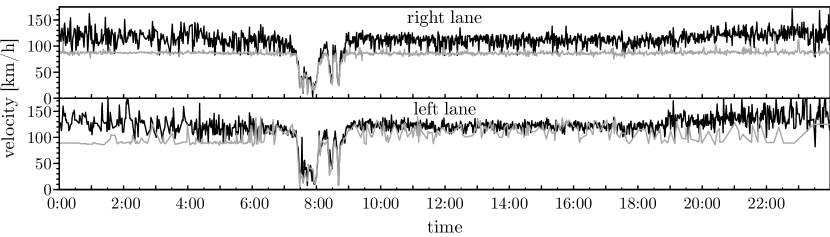
Figure 2: The velocity time series of detector D05 separated by lane and vehicle type. The time series of cars is depicted with a solid black line. The corresponding time series of trucks is depicted with a solid gray line. They are exemplary for all detectors upstream of the bottleneck. The breakdown occurs at approximately 7:15 a.m., it affects both lanes, and it lasts approximately $90\text{\,}\mathrm{min}\text{/}$. Microscopic traffic models should be able to reproduce this breakdown. (Missing data points, usually resulting from the lack of trucks in dilute traffic in the left lane, were approximated by a linear interpolation for better readability.)

By aggregating the same information as the real detectors, the simulations yield an equivalent set of data. To compare the resulting data, we propose two very intuitive approaches. Let $V_{\mathrm{e/s}}=\left\{v_{\mathrm{e/s}}(t_{1}),v_{\mathrm{e/s}}(t_{2}),...,v_{\mathrm{e/s}}(t_{n})\right\}$ signify the empirical (subscript e) and the simulated (subscript s) time series of a detector. By regarding the two sequences of length $n$ as $n$-dimensional vectors Brockfeld et al [19] suggested using the 1-norm $L_{1}$

$$L_{1}=\sum_{i=1}^{n}|v_{\mathrm{e}}(t_{i})-v_{\mathrm{s}}(t_{i})|$$ (2)

as a direct error measure. For the similarity analysis of two time series, however, the shape of the series is, in general, more important than their absolute values. Hence, random fluctuations in free traffic flow should be filtered and should not enter the comparison. Moreover, as the traffic models use different upper boundaries for vehicle velocities (see table 1), the resulting time series might have different amplitudes. Therefore, and according to [20], we suggested a normalization of the series before calculating the norm. The normalization of a time series $X=\left\{x_{1},x_{2},...,x_{n}\right\}$ with mean $\mu(X)$ and standard deviation $\sigma(X)$ is obtained by the affine transformation

$$x_{i}\rightarrow\frac{x_{i}-\mu(X)}{\sigma(X)}.$$ (3)

One should mention that the 1-norm is just one way of determining the distance between two time series. In general, any symmetric and positive-definite metric for which the triangle inequality holds could be applied.

Another promising method to assess the models’ quality is the study of the time series’ residuals. The residuals $R(t_{i})$ denote the difference between the observed and the simulated value at each time step $t_{i}$

$$R(t_{i})=v_{\mathrm{e}}(t_{i})-v_{\mathrm{s}}(t_{i}).$$ (4)

A classical approach to analyze time series is the decomposition of the series into three components [21]: a trend component, a seasonal component, and a noise component. If the model can reproduce the empirical data, the calculation of the residuals cancels the trend and seasonal components and leaves only the noise term. Under the assumption of white noise, the residuals are expected to behave randomly and to be uncorrelated. Similarly, it is also possible to determine the correlation between the two series. In this case, the degree to which the simulated time series reproduces the empirical data can be determined by the cross correlation of the two series.

4 Simulation setup

4.1 Models tested

For our analysis we restricted ourselves to the following three microscopic models for which asymmetric passing rules already exist: the Nagel-Schreckenberg model (NSM) [14], the comfortable driving model (CDM) [22, 23], and the intelligent driver model (IDM) [15].

The NSM and CDM are both traffic cellular automata (CA), where space and time are discrete, as explained earlier. It should be noted, though, that the newer CDM uses a finer discretization. In addition, the CDM was extended by some anticipatory components, which enable a vehicle to react more carefully to the preceding vehicle. The NSM, on the other hand, ignores any preceding vehicle, unless a collision is imminent. The IDM, in contrast, is a car-following model in continuous space and time. By a suited adaption to the preceding vehicle, the underlying differential equation leads to a very smooth driving behavior with realistic values of acceleration and deceleration. As the numerical evaluation of the IDM also requires a temporal discretization, the value of the temporal discretization in table 1 refers to the discretization that we used in our simulations. The NSM’s values were taken from [14, 24]. We did, however, double the length of slow vehicles to better mimic the physical properties of trucks. Analogously, we doubled the length of slow vehicles in the CDM. In contrast to Knospe et al[22, 23], we augmented the maximum velocity of both cars and trucks to obtain more realistic values with respect to a German Autobahn, but the absolute difference in maximum velocities was preserved.

Table 1: Comparison of the mobility models and the properties of vehicles in the respective model. In the case of asymmetric lane usage the IDM requires an additional parameter to model longitudinal motion. (The number in brackets refers to the symmetric case.) IDM’s parameters are taken from [25].

	unit	NSM	CDM	IDM
spatial discretization	[$\mathrm{m}\text{/}$]	$7.5$	$1.5$	$0.0$
temporal discretization	[$\mathrm{s}\text{/}$]	$1.0$	$1.0$	$0.25$
max. velocity car	[$\mathrm{m}\text{/}\mathrm{s}$]	$37.5$	$33.0$	$34.0\pm 20\%$
max. velocity truck	[$\mathrm{m}\text{/}\mathrm{s}$]	$22.5$	$25.5$	$23.0\pm 20\%$
max. acceleration	[$\mathrm{m}\text{/}{\mathrm{s}}^{2}$]	$7.5$	$1.5$	$1.5$
car length	[$\mathrm{m}\text{/}$]	$7.5$	$7.5$	$4.0$
truck length	[$\mathrm{m}\text{/}$]	$15.0$	$15.0$	$12.0$
additional parameters		$1$	$4$	$5(4)$

The single vehicle dynamics reveals the differences between the models. For each model, figure 3 shows the velocity profile of a vehicle starting at rest and approaching a parked vehicle $3\text{\,}\mathrm{km}\text{/}$ ahead. The discretization of the CA manifests itself in discontinuities of the corresponding velocity profile. The delayed acceleration in the CDM is due to a so-called slow-to-start rule. Due to this rule, a vehicle accelerates only with a given probability, when starting from rest. When approaching the parked vehicle, the IDM’s vehicle initiates a smooth braking process with realistic deceleration values. In the CA models, the vehicle comes to rest within one or two time steps (corresponding to $1\text{\,}\mathrm{s}\text{/}2\text{\,}\mathrm{s}\text{/}$) after driving at maximum speed. It has to be noted, however, that the resulting high deceleration rates can be observed in all models on roads with multiple lanes and on-ramps.

Figure 3: Velocity profiles for a vehicle starting from rest with a standing vehicle $3\text{\,}\mathrm{km}\text{/}$ ahead for the NSM, CDM, and IDM.

The asymmetric lane changing rules for the NSM are described in [26, 24]. (Several other asymmetric rule sets have been proposed. For an overview see the review article [1].) The CDM’s model description [22, 23] also provides the corresponding set of lane changing rules. A lane changing model for the IDM, called MOBIL, is given in [27, 25]. Referring to the cited articles, we will skip a detailed review of the models in favor of a precise description of the simulation setup.

4.2 Modeling open boundaries and ramps

The modeling of boundaries and ramps still offers several degrees of freedom and can significantly influence the resulting traffic patterns. Apart from the already mentioned boundary-induced phase transitions [28], the boundary setup can affect and limit the spectrum of observable traffic states [29].

Therefore, and for better reproducibility of our results, we want to give a concise description of the boundary and on-ramp setup. To insert new vehicles, we define an entrance section of length $l=x_{\mathrm{down}}-x_{\mathrm{up}}$, where $x_{\mathrm{down}}~{}(x_{\mathrm{up}})$ stands for the downstream (upstream) end of the entrance section. A vehicle entering the system adapts its velocity to the average velocity of the following and leading vehicles. The new vehicles is placed in the largest gap of the entrance section if the insertion is safe. The insertion is safe if neither the inserted vehicle’s deceleration nor the following vehicle’s deceleration falls below a threshold $b_{\mathrm{th}}=$-1\text{\,}\mathrm{m}\text{/}{\mathrm{s}}^{2}$$. (Due to the longitudinal-transversale coupling one has to check the other lane as well in the case of the IDM.) This strategy can be applied both to the on-ramp and to the upstream boundary.

Similarly, vehicles leaving the road via the off-ramp are selected from an exit section. The insert and exit sections representing the on-ramp and the off-ramp are restricted to the rightmost lane, whereas the upstream boundary’s entrance section spans both lanes.

To mimic the traffic state at the downstream boundary, we apply a dynamic speed limit from the position of detector D10 to the end of the road. The speed limit equals the maximum velocity that detector D10 measured during the previous aggregation interval. (As the CA models require an integer value for the speed limit, we converted the value by rounding it up.) To allow for a smooth deceleration with respect to the speed limit, we defined a deceleration section upstream of detector D10. Vehicles within the deceleration section gradually reduce their velocity such that they pass detector D10 with the desired velocity.

Vehicles are inserted according to the empirical data of detector D01. Consequently, the open boundary’s entrance section starts at the position of D01. For the length of the entrance section we used a value of $112.5\text{\,}\mathrm{m}\text{/}$, which is half the value we used for the on-ramp’s (off-ramp’s) entrance (exit) section. As there are no detectors directly measuring the vehicles entering or leaving the road via ramps, we determine these values by comparing the values of detectors D07 and D09 with each other. D07 (D09) is situated immediately downstream (upstream) of the off-ramp (on-ramp). If detector D09 measured more vehicles than D07, the surplus is inserted in the on-ramp section. Otherwise, the additional vehicles are removed from the exit section. In principle, it would also be possible to treat the D07- and D09-detector data separately. In this approach, however, we might remove a vehicle from the exit section and insert a new one in the entrance section at the same time. As each insertion represents a perturbation of traffic flow, which we want to minimize, this approach is less favorable. If an insertion or deletion fails, it is retried until it succeeds in conserving the total number of vehicles.

Moreover, trucks were not allowed to overtake in our simulation for two reasons. First, with asymmetric lane changing rules slower vehicles are required to stay in the right lane by legislation. Second, the examined road section is equipped with dynamic traffic signs which may impose an overtaking ban for trucks if traffic demand is high. Consequently, trucks were inserted only in the right lane at the upstream boundary. Figure 2 supports this assumption because the number of trucks detected in the left lane is quite low compared with the right lane.

4.3 Calibration

In contrast to previous works [5, 19, 30], we tried to avoid an automated model calibration, as an automated calibration not only questions the reliability of the obtained values [5] but can also produce parameter sets whose degree of realism can sometimes be doubted (see, e.g., the optimized parameter sets in [30]).

Due to various factors (e.g., weather, road characteristics, or different drivers), one cannot forgo a calibration completely though. As it might be quite instructive, we will briefly discuss the calibration steps we took. For the necessity of a calibration see figure 4, which shows the actual time series at detector D07 and the velocity time series of the uncalibrated models at the same position. As one can see, the NSM overestimates the severity of the breakdown, whereas the IDM does not show a breakdown at all.

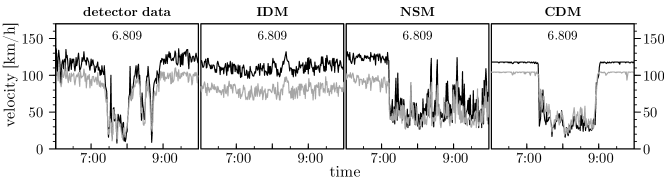
Figure 4: The empirical time series (left) and the time series produced by the three models with the original sets of parameters.

In the case of the NSM the calibration is obvious as the model has only one parameter left to calibrate (see table 1). This parameter controls the strength of fluctuations in traffic flow. Hence, we slightly reduced its initial value from $0.4$ to $0.32$. Despite its larger number of parameters, a calibration of the IDM was straightforward as well: we increased a driver’s desired time headway from $1.2\text{\,}\mathrm{s}\text{/}$ to $1.5\text{\,}\mathrm{s}\text{/}$. Thereby, we reduced the road’s effective capacity. (This change is still in good agreement with empirical data [31].) In this case, however, we found that many drivers were no longer able to enter the main road via the on-ramp due to the previously defined safety criteria. Therefore, we changed the threshold of the acceptable deceleration of following vehicles to $b_{\mathrm{th}}=$-50\text{\,}\mathrm{m}\text{/}{\mathrm{s}}^{2}$$. (Higher values of $b_{\mathrm{th}}$ did not yield satisfying results.)

5 Results

A first evaluation of the models’ behavior is best carried out by a graphical inspection of the resulting time series. Apart from the empirical time series, figure 5 shows the corresponding time series from several detector cross-sections for all models during the morning peak hour.

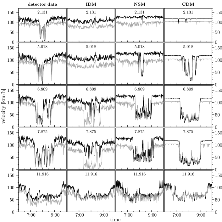
Figure 5: A comparison between empirical time series (first column) and the corresponding ones obtained with the IDM, NSM, and CDM (second to fourth column), respectively. From top to bottom the rows show the time series for D02, D04, D05, D06, and D10. The average velocities for the left (right) lane are plotted with a black (gray) line. Please note that, for the sake of clarity, we limited the depicted time to the interval from 6 a.m. to 10 a.m. Our analysis, however, is based on the time series of the entire day.

The empirical time series of detectors upstream of the bottleneck (i.e., D02 – D07) show a breakdown between 7:15 a.m. and 9:00 a.m. During this period, the average velocity on the faster left lane abruptly drops below the free flow velocity on the slower right lane and the velocity synchronizes across lanes. The temporal extent as well as the severity of the breakdown decreases with growing distance to the bottleneck (D06 $\rightarrow$ D02). Due to boundary effects detector D10 also shows a velocity synchronization with weaker fluctuations and a higher average velocity.

All models’ time series show good agreement with the empirical data at the downstream boundary (detector D10). This is, of course, a consequence of the dynamic speed limit which is imposed on the downstream (see section 4.2). Upstream of the bottleneck region, however, deviations between the models become obvious. The IDM’s time series does not show a synchronization between the two lanes. Although one can observe a breakdown in either lane, traveling in the left lane is always faster than in the right lane. This is a result of the very aggressive attitude ($b_{\mathrm{th}}=$-50\text{\,}\mathrm{m}\text{/}{\mathrm{s}}^{2}$$) with which drivers from the on-ramp enter the right lane of the main road. Greater values of $b_{\mathrm{th}}$, however, resulted in extinction of the breakdown. In contrast, both cellular automaton models reproduce the lane synchronization during traffic breakdown even for $b_{\mathrm{th}}=$0\text{\,}\mathrm{m}\text{/}{\mathrm{s}}^{2}$$. This follows from the models’ weaker safety constraints, which also result in the very unrealistic deceleration behavior observed in figure 3.

Another fundamental difference is the origin of velocity fluctuations in free traffic flow: the CDM and NSM incorporate random fluctuations by a stochastic component, whereas the fluctuations in the IDM result from the heterogeneity of the traffic (see table 1). For the first two models the strength of velocity fluctuations is governed by their spatial discretization, which explains why the fluctuations in the CDM’s time series are less pronounced than for the NSM.

As one can see from figure 5, the duration of the breakdown decreases in the upstream direction in both the empirical data and the data generated by the traffic models. All models underestimate the breakdown’s spatial extent though. At detector D02, free flow is restored in all models whereas empirical data still show the influence of the breakdown.

Similarly to the graphical inspection the numerical analysis does not reveal qualitative differences in the models’ velocity time series. Figures 6(a)–6(c) show the residuals’ autocorrelation for each model at detector D05, which is representative for the other detectors upstream of the on-ramp. Ideally, the residuals are uncorrelated, yielding an autocorrelation coefficient close to zero.

(a) IDM

(b) NSM

(c) CDM

(d) lane averaged correlation coefficients

(e) 1-norm

Figure 6: Autocorrelation of the time series’ residuals at detector D05 for the IDM 6(a), NSM 6(b), and CDM 6(c). Assuming white noise the $95\%$-confidence interval is plotted as a dashed horizontal line. The cross correlation between the empirical time series and the models’ time series is shown in 6(d). The 1-norm according to equation (2) is given in 6(e).

All models show a positive correlation ($>0.5$) for the residuals, which decreases with increasing time-lag. Hence, the assumption of white noise for the residuals has to be rejected. Figure 6(d) shows the correlation between the models’ time series and the empirical data. Due to the imposed downstream boundary conditions, the correlation coefficient’s maximum value ($>0.7$) is obtained at D10 for all models. For all models the correlation coefficient remains above $0.5$ up to detector D05 indicating a satisfying reproduction of the empirical data. The decrease in correlation with increasing distance to the ramps reflects the fact that all models do not successfully reproduce the spatial extent of the breakdown, as already discussed.

Probably the most intuitive comparison is obtained by the calculation of the 1-norm after transforming the time series according to equation (3). Remember that our primary quality criterion is the reproduction of the breakdown. Hence, we expect it to indicate to what extent the corresponding models achieve this goal. Figure 6(e) shows the 1-norm calculated for each detector and averaged over both lanes. At D02 (i.e., at kilometer $2.131$) the error for all models is about $1300$ (measured in arbitrary units) as all models fail to reproduce the breakdown at this position. Again, due to the boundary conditions, the best accordance with the empirical measurements is observed at detector D10. The qualitative behavior between detectors D01 and D10 is similar for all detectors. Even the absolute values of the NSM and the IDM are nearly identical; only the CDM’s values are considerably below the values of the previous models and indicate a better performance of this model.

5.1 Reproducibility of upstream boundary conditions

As we have seen, all investigated models are, in principle, able to reproduce the spatiotemporal traffic dynamics. As the simulations used the real detector data, it is worth discussing to what extent the empirical boundary conditions could actually be reproduced. In section 4.2 we described how vehicles were inserted and that a failed insertion had to be repeated in subsequent time steps until it succeeded. Of course, one would expect an insertion to always be successful as the empirical data prove that real traffic can satisfy the observed demand. In the simulations, we saw that insertions repeatedly failed especially during the peak hour period: table 2 gives the number of cars waiting for insertion or removal at the on-ramp or the off-ramp, respectively. Moreover, we have recorded the maximum time for either ramp during which the queue of vehicles waiting for insertion or removal was above zero. For instance, the maximum number of vehicles waiting for insertion in the NSM was 63 and the time span of a non-empty queue was $14\text{\,}\mathrm{min}\text{/}$.

Table 2: Overview of the usage of the on- and off-ramp queues

	max. queue length [veh] at		max. queue duration [$\mathrm{min}\text{/}$] at
model	on-ramp	off-ramp	on-ramp	off-ramp
IDM	139	41	82	22
NSM	63	42	14	9
CDM	55	42	10	41

These results confirm our previous statement that the safety conditions of the IDM make vehicle insertion more difficult. The maximum queue length for the IDM is twice as large as those for the two cellular automaton models. For all models, the queue length at the on-ramp reaches values considerably above zero. Whether a vehicle insertion fails depends on each model’s safety conditions. Moreover, the queue length’s growth reflects, at least partially, the fact that the models do not perfectly mimic human driving behavior. It has been found found, for example, in real traffic that the time headway of vehicles traveling at $110\text{\,}\mathrm{km}\text{/}\mathrm{h}$ can even drop below $0.5\text{\,}\mathrm{s}\text{/}$ [32]. Such values are impossible for all models due to their safety constraints. (In real traffic, such headways pose an actual risk, as drivers cannot react to actions of the preceding vehicle in a timely manner.)

5.2 Propagation velocity of breakdown

Another characteristic property of traffic flow is the propagation velocity of traffic jams and the shock (see section 2). Figure 5 shows that the breakdown propagates upstream. As the upstream and downstream fronts of a traffic jam are associated with sharp discontinuous changes of the average velocity, we define the time when the shock reaches the detector as the time when the average velocity first drops below a given threshold $v_{\mathrm{th}}$. Similarly, the time when the average velocity first exceeds $v_{\mathrm{th}}$ is considered as the detection of the downstream jam front. The numerical values of the propagation velocity of the shock and the traffic jam can be obtained from the quotient of the distance between subsequent detectors and the time that passed between the events being registered at either detector. In accordance with [33], we have set $v_{\mathrm{th}}=$30\text{\,}\mathrm{km}\text{/}\mathrm{h}$$. As the temporal resolution of one minute is relatively coarse, we averaged over the interval $v_{\mathrm{th}}=$ $30\pm 3\text{\,}\mathrm{km}\text{/}\mathrm{h}$ (see table 3).

Table 3: Averaged breakdown propagation velocities. The velocities are given in units of $\mathrm{km}\text{/}\mathrm{h}$.

	shock-wave velocity for				jam propagation velocity for
detectors	real data	NSM	IDM	CDM	real data	NSM	IDM	CDM
D07$\rightarrow$D06	-23	-7	-5	-2	-15	-17	-24	-9
D06$\rightarrow$D05	-12	-32	-14	-7	-11	-28	-3	-7
D05$\rightarrow$D04	-11	-3	NA	-3	-13	-3	NA	-3

Although the propagation velocities vary strongly between models and between successive detectors, all models correctly predict a negative propagation velocity (i.e., the breakdown moves upstream against the direction of traffic flow). Due to the relatively small inter-detector distances and due to an approximate error of $30\text{\,}\mathrm{s}\text{/}$ in the temporal determination of the breakdown, the error margins are quite large though. In principle, the error can be decreased by considering two detectors far away from each other (e.g., D07$\rightarrow$D02). For the empirical data set we found the propagation velocity to be $-13\text{\,}\mathrm{km}\text{/}\mathrm{h}$ for D07$\rightarrow$D02 and D06$\rightarrow$D02, which is in good agreement with the value of $-15\pm 2\text{\,}\mathrm{km}\text{/}\mathrm{h}$ found by Rehborn and colleagues [33].

5.3 Influence of truck length and the downstream boundary condition

Finally, we want to demonstrate the influence of vehicle length and the downstream boundary on our results. The vehicle length directly influences the spatial extent of the breakdown. Figure 7 shows the velocity time series from simulation runs where we increased the length of trucks by $7.5\text{\,}\mathrm{m}\text{/}1\text{\,}\mathrm{m}\text{/}1.5\text{\,}\mathrm{m}\text{/}$ for the NSM, the IDM, and the CDM, respectively. A comparison with figure 7 proves that this slight change of the vehicle properties results in a better agreement with the empirical data. For the NSM not only the spatial extent but also the temporal duration of the breakdown increases. Due to the NSM’s spatial discretization vehicle length can only be altered by multiples of $7.5\text{\,}\mathrm{m}\text{/}$.

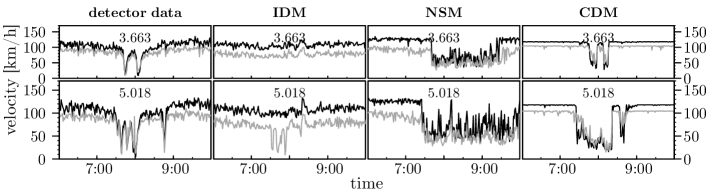
Figure 7: After increasing the length of trucks, the breakdown can be observed at detectors further upstream (cf. figure 5).

A more fundamental aspect is the nature of the breakdown. On the downstream boundary we had imposed a variable speed limit to mimic the velocities observed in real traffic. Hence, it is worth investigating whether the breakdown resulted from the imposed speed limit or whether it resulted from the vehicle interactions in the on-ramp region. Therefore, we repeated the simulations without the speed limit and, thereby, guaranteed free flow at the downstream boundary. The resulting exemplary time series for detector D06 is depicted in figure 8.

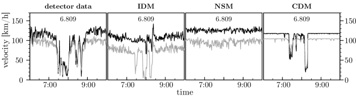
Figure 8: When modeling free flow at the downstream boundary, the intensity of the breakdown decreases in all models. For the NSM the breakdown even completely disappears.

The NSM’s time series no longer exhibits a breakdown, whereas the IDM and CDM still do. Consequently, the source of the breakdown in the NSM was our choice of the downstream boundary’s setup, whereas the breakdowns in the CDM and IDM are caused by the on-ramp boundary. However, also for the latter two models the shape of the time series changed: the breakdown’s duration decreased. Therefore, even if it does not select the traffic state (congested or freely flowing), the downstream boundary does determine its duration.

6 Conclusion

In this paper, we investigated the ability of three microscopic traffic models, namely the Nagel-Schreckenberg model (NSM), the comfortable driving model (CDM), and the intelligent driver model (IDM), to reproduce spatiotemporal traffic dynamics. To do so, we modeled a section of a German Autobahn with an off-ramp and an on-ramp. The inflow rates (via the upstream boundary and the on-ramp) and outflow rates (via the off-ramp) of vehicles were determined by the empirical traffic data that show a spontaneous breakdown during the morning peak hours. To assess our results and to compare the models with each other, we employed several methods known from time series analysis. We found that all models can reproduce the breakdown satisfyingly—at least after minor calibrations. Although the three models investigated here are microscopic ones, our observation is quite surprising as there are still substantial differences between the models (e.g., continuous versus discrete in space, realistic versus unlimited braking capacities, or deterministic versus stochastic approach).

Similarly, all models showed the same shortcomings. Compared with the empirical data, they underestimated the spatial extent of the breakdown. In real data, the breakdown could be detected more than $8\text{\,}\mathrm{km}\text{/}$ upstream of the on-ramp, which none of the models could reproduce. Therefore, we investigated the influence of the vehicles’ length on the traffic dynamics. We saw that the spatial extent of the breakdown can be effectively adjusted by the lengths of the different vehicle types.

Adjusting the length of vehicles, whose number is given by the boundary conditions, has a direct impact on the vehicle density and, thereby, on the probability with which vehicles can enter the road from the on-ramp. In this context, we did observe qualitative differences between the models though: in peak-hour traffic (i.e., high vehicle density), vehicles could more easily enter the main road via the on-ramp in the NSM and the CDM than in the IDM. The better reproduction of the empirical inflow rates exhibited by the CDM and NSM is a direct consequence of their unlimited braking capacity. The IDM, which shows a realistic deceleration behavior, makes higher demands on a safe entry and, therefore, it is more difficult for vehicles to enter in high density phases.

In contrast to the CDM and IDM, we found that the breakdown’s occurrence in the NSM did strongly depend on the modeling of the downstream boundary. Without applying a speed limit to the downstream boundary, we could no longer observe a breakdown in the NSM. From a physical point of view this is major difference between models. The consequences for practical applications, however, are less severe: for large scale traffic simulations (e.g., [34, 35]), the downstream boundary conditions are given by the traffic state of the neighboring road segment and cannot be chosen arbitrarily. Therefore, if the primary concern is the reproduction of the current traffic state, its physical origin may be of secondary importance.

As all models gave good results compared with the empirical data, is not possible to make a definite recommendation for one of them. The highest simulation speeds were observed with the NSM. Security-related aspects, which require a realistic acceleration and deceleration behavior, are best answered with the IDM. If the focus is rather on a realistic description of the spatiotemporal traffic dynamics, then the CDM is a good alternative. The authors, for example, recently studied the influence of inter-vehicle communication on traffic flow with the help of the CDM [36, 37]. In this context, the CDM offered a good combination for fast and realistic traffic simulations.

References

References

- [1] Debashish Chowdhury, Ludger Santen, and Andreas Schadschneider. Statistical physics of vehicular traffic and some related systems. Phys. Rep., 329(4-6):199–329, 2000.
- [2] Dirk Helbing. Traffic and related self-driven many-particle systems. Rev. Mod. Phys., 73(4):1067–1141, 2001.
- [3] Takashi Nagatani. The physics of traffic jams. Rep. Prog. Phys., 65(9):1331–1386, 2002.
- [4] Kai Nagel, Peter Wagner, and Richard Woesler. Still flowing: Approaches to traffic flow and traffic jam modeling. Oper. Res., 51(5):681–710, 2003.
- [5] Elmar Brockfeld, Reinhart Kühne, Alexander Skabardonis, and Peter Wagner. Toward benchmarking of microscopic traffic flow models. Transp. Res. Rec., 1852(1):124–129, 2003.
- [6] Sven Maerivoet and Bart De Moor. Cellular automata models of road traffic. Phys. Rep., 419(1):1–64, 2005.
- [7] Bernard Derrida and Martin R. Evans. Nonequilibrium Statistical Mechanics in One Dimension, chapter 14, pages 277–304. Camebridge University Press, Camebridge, 1997.
- [8] A. Schadschneider, D. Chowdhury, and K. Nishinari. Stochastic Transport in Complex Systems: From Molecules to Vehicles. Elsevier Science, Oxford, UK, 2010.
- [9] Anatoly B. Kolomeisky, Gunter M. Schütz, Eugene B. Kolomeisky, and Joseph P. Straley. Phase diagram of one-dimensional driven lattice gases with open boundaries. J. Phys. A: Math. Gen., 31(33):6911, 1998.
- [10] V. Popkov and Gunter M. Schütz. Steady-state selection in driven diffusive systems with open boundaries. Europhys. Lett., 48(3):257, 1999.
- [11] T. Antal and G. M. Schütz. Asymmetric exclusion process with next-nearest-neighbor interaction: Some comments on traffic flow and a nonequilibrium reentrance transition. Phys. Rev. E, 62:83–93, 2000.
- [12] J. S. Hager, J. Krug, V. Popkov, and G. M. Schütz. Minimal current phase and universal boundary layers in driven diffusive systems. Phys. Rev. E, 63:056110, 2001.
- [13] Wolfgang Knospe, Ludger Santen, Andreas Schadschneider, and Michael Schreckenberg. Empirical test for cellular automaton models of traffic flow. Phys. Rev. E, 70(1):016115, 2004.
- [14] Kai Nagel and Michael Schreckenberg. A cellular automaton model for freeway traffic. J. Phys. I, 2(12):2221–2229, 1992.
- [15] Martin Treiber, Ansgar Hennecke, and Dirk Helbing. Congested traffic states in empirical observations and microscopic simulations. Phys. Rev. E, 62(2):1805–1824, 2000.
- [16] Vladislav Popkov, Ludger Santen, Andreas Schadschneider, and Gunther M. Schütz. Empirical evidence for a boundary-induced nonequilibrium phase transition. J. Phys. A, 34(6):L45, 2001.
- [17] Boris S Kerner, Sergey L Klenov, and Andreas Hiller. Empirical test of a microscopic three-phase traffic theory. Nonlinear Dyn., 49(4):525–553, 2007.
- [18] Boris S. Kerner and Sergey L. Klenov. Phase transitions in traffic flow on multilane roads. Phys. Rev. E, 80:056101, 2009.
- [19] Elmar Brockfeld and Peter Wagner. Calibration and validation of microscopic traffic flow models. In Serge P. Hoogendoorn, Stefan Luding, Piet H. L. Bovy, Michael Schreckenberg, and Dietrich E. Wolf, editors, Traffic and Granular Flow ’03, pages 67–72. Springer, Berlin, 2005.
- [20] Dina Goldin and Paris Kanellakis. On similarity queries for time-series data: Constraint specification and implementation. In Ugo Montanari and Francesca Rossi, editors, Principles and Practice of Constraint Programming — CP ’95, volume 976 of Lecture Notes in Computer Science, pages 137–153. Springer, 1995.
- [21] Henrik Madsen. Time Series Analysis. Chapman and Hall/CRC, 2007.
- [22] Wolfgang Knospe, Ludger Santen, Andreas Schadschneider, and Michael Schreckenberg. Towards a realistic microscopic description of highway traffic. J. Phys. A, 33(48):L477, 2000.
- [23] Wolfgang Knospe, Ludger Santen, Andreas Schadschneider, and Michael Schreckenberg. A realistic two-lane traffic model for highway traffic. J. Phys. A, 35(15):3369, 2002.
- [24] Wolfgang Knospe, Ludger Santen, Andreas Schadschneider, and Michael Schreckenberg. Disorder effects in cellular automata for two-lane traffic. Physica A, 265:614–633, 1999.
- [25] Arne Kesting, Martin Treiber, and Dirk Helbing. General lane-changing model mobil for car-following models. Transp. Res. Rec., 1999:86–94, 2007.
- [26] Martin Rickert, Kai Nagel, Michael Schreckenberg, and A. Latour. Two lane traffic simulations using cellular automata. Physica A, 231(4):534 – 550, 1996.
- [27] Martin Treiber and Arne Kesting. Modeling lane-changing decisions with mobil. In Cécile Appert-Rolland, François Chevoir, Philippe Gondret, Sylvain Lassarre, Jean-Patrick Lebacque, and Michael Schreckenberg, editors, Traffic and Granular Flow ’07, pages 211–221. Springer, 2009.
- [28] Joachim Krug. Boundary-induced phase transitions in driven diffusive systems. Phys. Rev. Lett., 67(14):1882–1885, 1991.
- [29] Robert Barlovic, Torsten Huisinga, Andreas Schadschneider, and Michael Schreckenberg. Open boundaries in a cellular automaton model for traffic flow with metastable states. Phys. Rev. E, 66(4):046113, 2002.
- [30] Vincenzo Punzo and Fulvio Simonelli. Analysis and comparison of microscopic traffic flow models with real traffic microscopic data. Transp. Res. Rec., 1934(1):53–63, 2005.
- [31] Arne Kesting and Martin Treiber. Calibrating car-following models by using trajectory data: Methodological study. Transp. Res. Rec., 2088:148–156, 2008.
- [32] Cécile Appert-Rolland. Experimental study of short-range interactions in vehicular traffic. Phys. Rev. E, 80:036102, 2009.
- [33] Hubert Rehborn, Sergey L. Klenov, and Jochen Palmer. Common traffic congestion features studied in USA, UK, and Germany based on Kerner’s three-phase traffic theory. In IEEE Intell. Veh. Symp., pages 19–24, 2011.
- [34] Sigurdur Hafstein, Roland Chrobok, Andreas Pottmeier, Michael Schreckenberg, and Florian Mazur. A high-resolution cellular automata traffic simulation model with application in a freeway traffic information system. Comput.-Aided Civ. Infrastruct. Eng., 19(5):338–350, 2004.
- [35] Traffic information system “autobahn.nrw”. http://www.autobahn.nrw.de/, 2011.
- [36] Florian Knorr and Michael Schreckenberg. Influence of inter-vehicle communication on peak hour traffic flow. Physica A, 391(6):2225 – 2231, 2012.
- [37] Florian Knorr, Daniel Baselt, Michael Schreckenberg, and Martin Mauve. Preventing traffic jams via vanets. IEEE Trans. Veh. Technol., 61, 2012.