P/2010 A2 LINEAR

P/2010 A2 is an object on an asteroidal orbit that was observed to have an extended tail or debris trail in January 2010. In this work, we fit the outburst of P/2010 A2 with a conical burst model, and verify previous suspicions that this was a one–time collisional event rather than an sustained cometary outburst, implying that P/2010 A2 is not a new Main Belt Comet driven by ice sublimation. We find that the best–fit cone opening angle is $\sim 40^{\circ}$ to $\sim 50^{\circ}$ , in agreement with numerical and laboratory simulations of cratering events. Mapping debris orbits to sky positions suggests that the distinctive arc features in the debris correspond to the same debris cone inferred from the extended dust. From the velocity of the debris, and from the presence of a velocity maximum at around $15\rm\,cm\,s^{-1}$, we infer that the surface of A2 probably has a very low strength ($\lesssim 1\,\rm kPa$), comparable to lunar regolith.

1 Introduction

P/2010 A2 was discovered by LINEAR (Birtwhistle et al. 2010a) on 7 Jan 2010 on an orbit typical of a Main Belt asteroid, with a Tisserand parameter $T_{J}=3.6$ and orbital elements suggesting it belongs to the Flora collisional family. At the time of discovery, it appeared as “a headless comet with a straight tail, and no central condensation” (Birtwhistle et al. 2010b). A few days later, observers reported an asteroid-like body connected to the tail by a narrow light bridge (Green 2010). Jewitt et al. (2010a) and Licandro et al. (2010) interpreted the detached nucleus as the consequence of an impact.

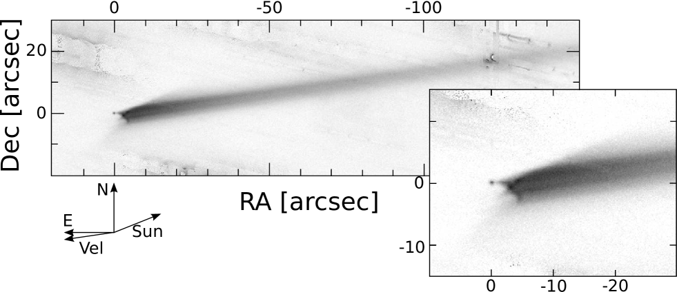
Figure 1: P/2010 A2, images from UT 19.5 Jan 2010 using Gemini North. The linear gray scale covers the range of (0–3) $\times 10^{-8}Af$ (a dust proxy; see Paper I, Section 3.3.3). The positions of North (N) and East (E) are indicated, as are the anti-solar direction and the heliocentric velocity vector. From Paper I, Figure 2.e.

Moreno et al. (2010) observed the comet with the Gran Telescopio Canarias, the William Herschel Telescope, and the Nordic Optical Telescope on La Palma. They modeled the observed tail using water-driven cometary activity extending over a period of several months.

Jewitt et al. (2010b) acquired a series of observations with the Hubble Space Telescope over a long period from January to May 2010. The nucleus appears not to be immediately surrounded by dust, which is further confirmed by a fairly constant absolute magnitude over the span of their observations. The detached tail is a narrow trail, striped with very narrow, parallel striae that emanate from two sharp arcs crossing to form a X. From the evolution of the tail geometry, in particular its orientation, they concluded that the dust release occurred during a very short event that took place in Feb.–Mar. 2009. They suggest that this event was caused either by a collision or a spin up of the nucleus.

Snodgrass et al. (2010) acquired images of P/2010 A2 using the camera onboard the Rosetta space probe. The very different —and favourable– viewing geometry allowed them to constrain accurately the dust release period to a very short burst around 10 Feb 2009.

We acquired a series of ground-based images using Gemini North and the University of Hawai‘i 2.2-m telescope on Mauna Kea, and the ESO New Technology Telescope on La Silla. The observations, data processing and overall analysis are presented in Hainaut et al. (2011, hereafter Paper I). Figure 1 shows the deepest image of the series. The Gemini observations, which combined a very sharp image quality with very deep surface brightness sensitivity, further confirm that the nucleus is devoid of nearby dust. Assuming an albedo of $p=0.11$ and a solar phase correction $G=0.15$ (values typical for S-type asteroids, the most frequent members of the Flora family), its magnitude converts to a radius $r=80$–$90\,\rm m$, in agreement with the values reported by Moreno et al. (2010), Jewitt et al. (2010b) and Snodgrass et al. (2010).

The analysis included thermal modelling of the nucleus, which ruled out the presence of any water ice (as well as all more volatile species) down to the center of the object, provided it remained on its current orbit for more than a few million years. As there is no reason to suspect that P/2010 A2 has been recently injected into its orbit, this excludes cometary activity as the source of the dust release.

The data presented in Paper I also show the features observed by Jewitt et al. (2010b); they are summarized in Fig. 2. The tail-like dust trail was analyzed using the Finson & Probstein (1968) method, constraining the dust release to a short period of time about one year before the observations. This modelling, combined with direct measurements of the tail, indicate that the dust grains had radii $a$ in the mm to cm range, with a size distribution in $a^{\sim-3.5}$, and that the tail contained over $8\times 10^{8}$ kg of dust, assuming a density $\rho=3\,000$ kg m^-3 (typical value for a S-type asteroid).

More advanced dust dynamical models were developed to investigate the origin of the dust emission. While Paper I summarized the main features of these models, this paper describes them in detail. Sections 2 and 3 describes the models used to study the overall envelope of the dust trail, while Section 4 is devoted to the analysis of the X-shape arcs, labeled Arc 1 and 2 in Fig. 2.

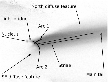
Figure 2: Schematic of the main features of P/2010 A2, from Paper I.

2 Modeling the dust distribution - a simple binary envelope fit

Our principal aim is to determine whether a simple single–burst model can account for the most salient features of the P/2010 A2 outburst, and whether a burst corresponding to a collision event fits the data. A general single–burst model consists of an arbitrary differential distribution of dust particles of solar radiation pressure coefficient $\beta$ and velocity vector ${\bf v}_{\rm d}$, given by $f({\bf v}_{\rm d},\beta)\,d{\bf v}\,d\beta$.

Various approaches have been used for this type of general dust and debris fitting. For example, Jorda et al. (2007) modeled the Deep Impact ejecta cone using a $\chi^{2}$ fit of a set of synthetic image components, and obtained the dust size and velocity distributions. Deep Impact had the advantage of a known ejecta geometry; if this procedure were repeated with a completely unknown geometry, the problem would become intractable using this image superposition method, because the number of input images would be multiplied by the number of possible geometries. Moreover, the relatively clean and low noise dataset of Deep Impact permitted the use of a quadratic (Gaussian) fit, which is amenable to linear solutions.

Moreno (2009) modeled comet 29P/Schwassmann–Wachmann using a similar linear approach, finding that a simplified set of emission regions combined with rotation gave a better fit than fixed sunward emission.

We elect not to use these superposition methods for several reasons. Because we wish to reconstruct the emission direction, we cannot assume a direction like Jorda et al. (2007). A completely general superposition solution permitting emission in cones spaced at $10^{\circ}$ intervals in latitude and longitude, with 10 opening angles, 10 velocities, and 10 dust sizes would require solving for over half a million linear coefficients, an intractable computation because linear problems scale with the cube of the number of components. Even if this were computable, it would be necessary to impose normalization (smoothness) conditions that would dominate any solution.

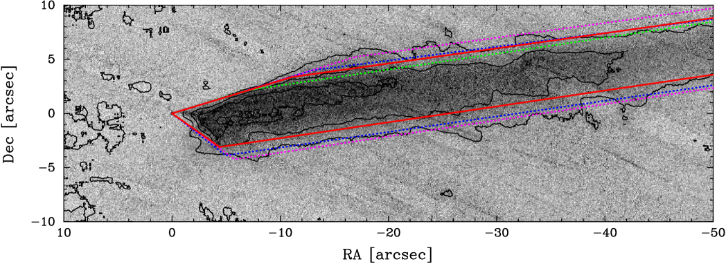
Figure 3: Our best estimate (solid red line) of the dust envelope superimposed on the 29 Jan 2010 HST image, along with three other plausible envelopes (dotted lines in blue, green, and magenta). The isophotal contours (black) are in rough agreement with the envelopes. The envelopes fit equally well on our Gemini image (Fig. 1).

Thus, instead of undertaking a general fit, we elect to fit a much less complicated parametric model. Our first simplification is to assume that the outburst is a single hollow cone, with an opening half–angle $\alpha_{c}$; for example, $\alpha_{c}=0$ corresponds to a thin pencil–beam of debris. Such cones are typical of impact ejecta (see Richardson et al. (2007), hence R2007, and Holsapple (1993) for overviews). We define a right–handed orthogonal coordinate system $(x_{A2},y_{A2},z_{A2})$ such that the nucleus is at the origin, $x_{A2}$ points away from the Sun, $y_{A2}$ is in the orbital plane and points in the sense of the orbital motion, and $z_{A2}$ points out of the orbital plane. There are corresponding polar coordinates $\phi_{A2}$, the latitude angle from the orbital plane toward $z_{A2}$, and $\theta_{A2}$, the angle in the $x_{A2},y_{A2}$ plane starting in the $+x_{A2}$ direction. For example, the direction $\phi_{A2}=90^{\circ}$ points at the $+z_{A2}$ pole, and $\theta_{A2}=90^{\circ},\phi_{A2}=0^{\circ}$ points in the $+y_{A2}$ direction.

Our second simplification is to disregard completely the intensity of the dust distribution, and consider only whether it fills the apparent dust envelope of the observations (i.e., a binary fit). This means that we may ignore the distributions of the dust size and velocity, and consider only their minimum and maximum values. By setting the minimum velocity and dust size to be zero, assuming that dust size is independent of velocity, and assuming that the minimum dust size escapes beyond the fitting region, these four parameters reduce to the single parameter of maximum dust velocity. Hence the fitting procedure is reduced to four dimensions: $\alpha_{c},\phi_{A2},\theta_{A2},{v_{\rm d}}_{\rm max}$.

Our code contains two orbit integrators: a conventional Runge-Kutta stepper, which takes the gravity of the nucleus into account but is slow; and an exact Keplerian solver that integrates the orbit in a single step, but sees only the Sun’s gravity and solar pressure. Tests revealed that adjusting the ejection velocity by an assumed escape velocity $v_{e}\sim 10\,{\rm cm\,s^{-1}}$ (Hainaut et al. 2011), according to $v_{\rm final}=\left({v_{\rm ejection}}^{2}-{v_{e}}^{2}\right)^{1/2}$ brought the Keplerian variant into very close observational agreement with the full Runge-Kutta integrator, so the faster Keplerian code was used throughout, even when taking into account the mass of the nucleus.

The fitting procedure is then to assume the outburst date of Snodgrass et al. (2010), 10 Feb 2009 ($\pm 5$ days). We create a conical burst with a particular set of parameters $\alpha_{c},\phi_{A2},\theta_{A2},{v_{\rm d}}_{\rm max}$, integrate it to the date of the observations, create a model image, and evaluate the goodness of fit to the actual image. The penalty function of the fit consists of $+1$ for each pixel of the model image that falls outside the observed dust envelope, and $+1$ for each pixel inside the observed envelope that is dust-free. For pixels that fall within $20\arcsec$ of the nucleus, we multiply the penalty by 10, to enforce a good fit of the corner features at the cost of being lax with the distant tail. If the model dust perfectly fills the envelope, and no dust falls outside, the penalty is zero.

The observed envelope is determined by finding, by eye, the limits of the dust in the 29 Jan 2010 Hubble Space Telescope (HST) image and drawing a polygonal fit to them (Fig. 3).. This procedure is admittedly imprecise and somewhat arbitrary, but the main envelope drops down sharply to the apparent sky level, so there is only modest latitude in drawing the envelope, neglecting the diffuse features (Fig. 2) in the first part of the analysis. Furthermore, our purpose is to perform a simplified fit to show the plausibility of a single simple burst event creating features similar to those seen in P/2010 A2, not to perform the far more difficult task of an exact fit to the outburst. The main features that we try to explain are the bottom sharp corner of the dust envelope, $4\aas@@fstack{\prime\prime}4$ south and $3\aas@@fstack{\prime\prime}1$ west of the nucleus, and a gentler bend $3\aas@@fstack{\prime\prime}6$ to the north and $11\aas@@fstack{\prime\prime}1$ to the west, with the envelope converging from these bends to a point at the nucleus and extending in a broad tail to the west. That is, we represent the envelope as a five–sided polygon. Figure 3 shows our best estimate of the envelope superimposed on the HST image, as well as three other plausible envelopes to test the sensitivity of our conclusions on the subjectivity of the envelope.

2.1 General behavior of the conical burst model

As a first experiment in how debris models can vary in appearance, we integrate models with fixed $\alpha_{c}=45^{\circ}$ and ${{v_{\rm d}}_{\rm max}}=33\,{\rm cm\,s^{-1}}$ in a set of $\phi_{A2},\theta_{A2}$ directions consistent with the directions of a cube in $(x_{A2},y_{A2},z_{A2})$ space. There are $3^{3}-1=26$ such directions, made up of all permutations of $(x,y,z)$ with $x,y,z\in\left\{-1,0,+1\right\}$ excepting $(0,0,0$). For instance, the direction $(1,1,1)$ corresponds to $\phi_{A2}=\theta_{A2}=45^{\circ}$.

Figure 4 shows this ensemble of models. In each sub–plot, the red arrow indicates the projected direction to the sun, the blue arrow is the vector out of the orbital plane, and the green arrow is the orbital direction. Solid (dotted) vectors point out of (into) the page. The orange dots correspond to some more obvious streaks and boundaries of the observed dust distribution; these are not the dust envelope used in the actual fit in the subsequent section.

Figure 4 demonstrates that a wide range of morphologies can be produced by varying only the ejection direction. The sharp bends that are seen in the actual data are observed in many of the models, and result from sheet–like or slab–like configuration of the final dust distribution, with the boundary of the slab determined by the maximum dust velocity.

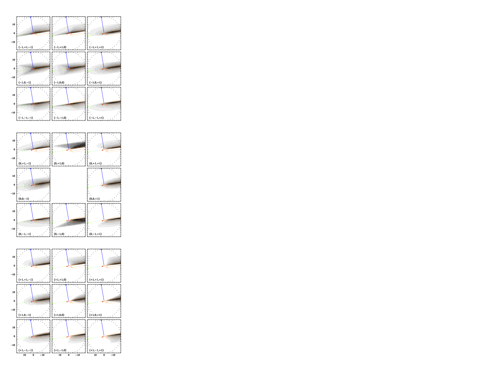
Figure 4: Dust simulations of a single conical eruption with fixed maximum velocity ${v_{\rm d}}_{\rm max}=33{\rm cm\,s^{-1}}$ and cone angle $\alpha_{c}=45^{\circ}$ but with varying emission direction, as described in Sec. 2.1. Units are arcseconds in RA (abscissa) and Dec (ordinate), in the usual N–up, E–left orientation.

2.2 Fitting procedure and results

Because small changes in the geometry lead to large changes in the appearance of the model, and because the penalty function of the fit is not smoothly varying and may possess multiple minima, we employ a two–dimensional downhill simplex minimizer described in Press et al. (1992), running over a grid of the two remaining variables. Specifically, we freeze $\alpha_{c}$ and $\phi_{A2}$ over a $10^{\circ}$ mesh of discrete values, and optimize only in the two dimensions $\theta_{A2},{v_{\rm d}}_{\rm max}$. This particular optimization scheme is motivated by several considerations: First, ${v_{\rm d}}_{\rm max}$ represents a stable and smooth rescaling of envelope size, and may be safely placed inside the simplex optimizer. Next, the cone angle $\alpha_{c}$ is of physical interest, so the method should produce contours in it. Finally, the dust envelope varies unpredictably with the remaining parameters $\phi_{A2}$ and $\theta_{A2}$, so that not more than one of them should be placed into the simplex optimizer in order to avoid false local minima.

We find that positive values of $\phi_{A2}$ do not fit the bottom portion of the envelope at all, successfully filling only the top portion of the tail, and sometimes explaining the northern bend, as seen in some panes of Fig. 4. Similarly, negative values of $\phi_{A2}$ with small opening angles $\alpha_{c}$ can fit the bottom bend of the envelope, and fill the bottom part of the tail, but fail to account for the top bend. Large ($\alpha_{c}>50^{\circ}$) opening angles tend to produce east–projecting spines of dust that are not seen in the actual data. However, a model with a cone angle $\alpha_{c}=40^{\circ}$ and $\phi_{A2}=-20^{\circ}$, with best–fit values ${v_{\rm d}}_{\rm max}=0.2\,\rm ms^{-1}$ and $\theta_{A2}=74^{\circ}$, produces good visual agreement with the dust envelope, as well as the smallest value of the penalty function. The bend in the bright envelope around the “North diffuse feature” of Fig. 2 arises naturally as a consequence of the edge of the cone, blown backward by radiation pressure.

Figure 5 shows penalty function contours in $\alpha_{c}$ and $\phi_{A2}$; the contours are very similar for the various assumed envelopes of Fig. 3. Figures 7a to e illustrate the best fit model, as well as models that optimize $\theta_{A2}$ and ${v_{\rm d}}_{\rm max}$, but are away from the best $\phi_{A2}$ and $\alpha_{c}$. Repeating the process using a solid rather than hollow conical burst gives the same best model, because the two cone types differ only though the presence of a spherical instead of planar end–cap.

In addition to performing the minimization by fixing $\alpha_{c},\phi_{A2}$, we also ran an optimization over a grid of fixed $\theta_{A2},\phi_{A2}$. Figure 6 shows that there is a second good fit value at $\theta_{A2}\approx 0^{\circ},\phi_{A2}\approx-20^{\circ}$, with a similar cone opening angle as the first solution. Therefore, we must keep in mind that our first solution is degenerate with a second slightly worse solution. The two solutions are related in a physically straightforward manner, evident upon viewing the model in three dimensions: in one solution, one side of the cone agrees with the direction of solar pressure, so that particles in this direction remain on a concentrated stream rather than being dispersed, and the opposite side of the cone points at the observer, and is dispersed by sunlight. In the other solution, the cone is rotated by nearly $90^{\circ}$ (two cone half-opening angles), and debris on the other side of the cone remains coherent, while the first side points away from the observer is dispersed. The existence of two solution differing by roughly a right angle is thus an independent argument for a $\alpha_{c}\approx 45^{\circ}$ cone. In each case, the main central streak extending from the nucleus can be interpreted as the region of the cone over which a spread in velocities does not result in a transverse (to the stream) spread in position. It may be that this alignment helped P/2010 A2 become visible in the first place, because the brightest features of the object appear to coincide with fortuitous line–of–sight alignments down the long axis of the dust cone.

In summary, we found two solutions for the parameters, with $\theta_{A2}\approx 74^{\circ}$ or $\sim 0^{\circ}$, both with a cone half opening angle of $\alpha_{c}\approx 45^{\circ}$ and a maximum velocity of $20$ to $30\,\rm cm\,s^{-1}$. The two solutions correspond to a rotation of the cone by its full width. Because this is not a $\chi^{2}$ fit, formal uncertainties cannot be provided. From plots of the simplex–optimized models on the $\phi_{A2},\alpha_{c}$ grid, we conclude that only models with $30^{\circ}\lesssim\alpha_{c}\lesssim 50^{\circ}$ and $10^{\circ}\lesssim\phi_{A2}\lesssim 30^{\circ}$ plausibly fill the dust envelope, providing approximate constraints for these two parameters. Models outside the third contour of Fig. 5 do not appear correct (e.g. Fig. 7d).

Figure 5: Contours of the binary penalty function in the space of the cone opening angle $\alpha_{c}$ and the latitude direction of ejection $\phi_{A2}$, after optimizing over $\theta_{A2}$ and ${v_{\rm d}}_{\rm max}$. The left panel is the fit for the best estimate of the envelope, and the right panel is the most discordant (green) fit from the envelopes in Figure 3. Units are arbitrary, and there is no statistical interpretation of the contour values because they are not $\chi^{2}$ values. For the best envelope, there is a clear optimum at $\phi_{A2}=-20^{\circ}$ and $\alpha_{c}=40^{\circ}$, denoted by a plus symbol. The optimum is shifted only slightly for other assumed envelopes.

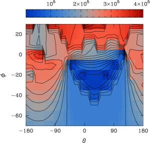
Figure 6: Left: Contours of the binary envelope penalty function in $\theta,\phi$, with the largest plus symbol indicating the minimal value, and the other symbols indicating the next two best values. The best solutions are seen to exist in two degenerate islands. Right: The remaining free parameters $\alpha_{c}$ and $v_{\rm max}$ as a function of the penalty. The two islands of solutions give similar values for both parameters, so the choice of solution does not affect the physical interpretation of the event, beyond the direction.

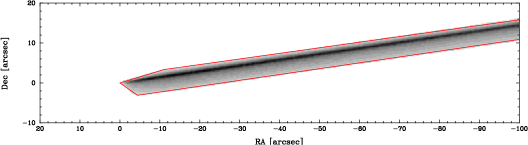
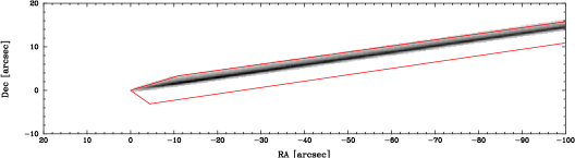
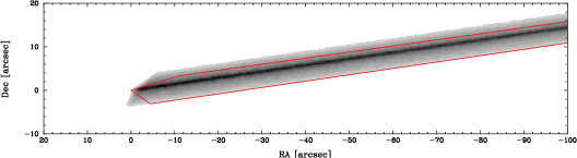
a) b) c) d) e)

Figure 7: a) The best hollow cone model, filling the estimated P/2010 A2 dust envelope (red). This model consisted of a cone with an opening angle $\alpha_{c}=40^{\circ}$, pointing downward at $\phi_{A2}=-20^{\circ}$ and forward at $\theta_{A2}=74^{\circ}$, with a maximum dust velocity ${v_{\rm d}}_{\rm max}=0.2\,\rm ms^{-1}$. The central streak is the zero–velocity component of the dust distribution. b) A hollow cone model with a thin cone $\alpha_{c}=10^{\circ}$ and $\phi_{A2}=-30^{\circ}$. Many thin cone models pointing downward successfully fill the bottom part of the envelope, but do not account for the top. c) A hollow cone model with a thin cone $\alpha_{c}=10^{\circ}$ and $\phi_{A2}=+10^{\circ}$. Models with $\phi_{A2}=>0^{\circ}$ tend to fill or overfill the top part of the envelope, but leave the bottom part empty. d) A broad cone with $\alpha_{c}=80^{\circ}$ and $\phi_{A2}=-20^{\circ}$ tends to overfill the envelope, producing a spur on the left, and fails to match the top contour of the envelope. e) A broad cone $\alpha_{c}=60^{\circ}$ pointing downward at $\phi_{A2}=-80^{\circ}$. Models with $\phi_{A2}=<-50^{\circ}$ tend to produce east projecting dust, and very broad cones tend to overfill the envelope at some points in order to fill it at others.

3 Modeling the general dust envelope - a multiparametric fitting approach

The dust fitting approach of §2 relied on a hand–drawn trace of the dust envelope, based on the isophotes of the images. It possesses the advantages of fitting speed, fit robustness, and simplicity, but has the drawback of subjectivity. To address this concern, we constructed a more complex model with a non-binary fit, fitting the observed dust profile, after modelling the emission with a set of power laws.

Specifically, we assume that the initial differential dust distribution in dust $\beta$ and velocity $v_{d}$, before applying an escape velocity $v_{e}$, is given by

$$N(\beta,v_{d})\propto\Theta\left(v_{0}(\beta/\beta_{0})^{\delta}-v_{d}\right)\times{v_{d}}^{\nu}\beta^{\gamma}$$ (1)

In this equation $\Theta\left(v_{0}(\beta/\beta_{0})^{\delta}-v_{d}\right)$ is the Heaviside step function that truncates the maximum velocity as a powerlaw $(\beta/\beta_{0}^{\delta})$, where $\beta_{0}=10^{-5}$ is fixed. Within this truncation, the dust velocity is a powerlaw in velocity $N\propto{v_{d}}^{\nu}$, and a powerlaw in dust size $N\propto\beta^{\delta}$.

It is useful to examine the observational implication of each parameter: $\gamma$, the dust exponent, determines the fading of the trail along its long axis. $\nu$, the velocity exponent, determines the profile of the trail in the direction of ejection, and its effect is co–mingled with the effects of geometry and light pressure. $\delta$, by truncating the velocity in a manner that depends on $\beta$, controls the broadening of the trail as it extends from the nucleus, because smaller and more distant dust particles are ejected faster. $v_{0}$ sets the limiting envelope of the dust trail. Finally, the escape velocity $v_{e}$ depopulates regions close to the nucleus (and by extension the center of the trail) by remapping the low velocity dust distribution according to $v_{\rm final}=\max\left(0,{v_{d}}^{2}-{v_{e}}^{2}\right)^{1/2}$. Thus this parameterization, even if it does correspond perfectly to underlying physics, captures many of the observational variables of the system.

The truncation in velocity is similar to Jorda et al. (2007), which is based on O’Keefe & Ahrens (1985), who find that maximum debris velocity is truncated for a given particle mass as $v_{\rm max}\propto m^{-1/2}$ to $m^{-1/6}$ with the best fit being $m^{-1/3}$. From the fact that $\beta$ is inversely proportional to the dust radius, it is true that $\beta\propto m^{-1/3}$, implying that $\delta\in[0.5,1.5]$, with $\delta=1$ corresponding to the best fit of O’Keefe & Ahrens (1985). However, we caution that this form of the truncation is based on fragmentation assumptions, and it is not obviously applicable to a loose regolith. In fact, the value of $\delta$ inferred from the literature appears inapplicable to this system, because $\beta$ spans values of $10^{-6}$ to $10^{-4}$ between 0″and 150″from the nucleus, implying that the envelope of the tail must expand by a factor of at least 10 (for $\delta=0.5$) from the nucleus to the boundary of our images. From inspection of the images, the trail does not appear to broaden by this much, although the broadening may occur in a faint and invisible halo outside the visible envelope.

For the differential size $a$ distribution of particles, Paper I found $dN/da\propto a^{-3.5}$, similar to the analytical result for a relaxed population (Dohnanyi 1969). This corresponds to a distribution $dN/d\beta\propto\beta^{\gamma}$ for $\gamma=1.5$.

O’Keefe & Ahrens (1985) find that the fraction of mass ejected below a particular velocity $v$ is given approximately by $M/M_{\rm Total}\approx 1-v^{-1.3}$, so that the differential exponent $\nu\approx-2.3$ as long as the particle velocity is independent of particle size.

The penalty function of the multi–parameter fit, instead than being binary as in §2, uses the absolute difference of the predicted image with the observed image as the fit metric: ${\rm Penalty}=\left|{\rm Image}-{\rm Model}\right|\times\left(1+(R/R_{0})^{2}\right)^{-\eta}$, where $R$ is the distance from the nucleus in arcseconds and $R_{0}$ is a scale parameter. We use a robust absoute deviation penalty rather than the more common quadratic one, because a quadratic fit is strictly correct only for known Gaussian uncertainties, whereas our images are dominated by unknown systematics. Additionally, the penalty is scaled by a $\left(1+(R/R_{0})^{2}\right)^{-\eta}$ weighting function centered on the nucleus to suppress the fit at large radii and prevent noise features in the image from dominating, because most of the image area is background, far from the nucleus and away from the trail. The final fit values are insensitive to $R_{0}$ between $7\arcsec$ to $30\arcsec$, and $\eta\in[0.5,1]$, though smaller values of $R_{0}$ experience more reliable fit convergence.

To perform the fit, we optimized over a grid of fixed $\theta_{A2},\phi_{A2}$, and used Powell’s method (Press et al. 1992) because it is better suited for the smooth powerlaw parameters than the previous downhill simplex.

Figure 8 (left) shows the resulting penalty contours in $\theta_{A2},\phi_{A2}$. Although not as clean as in the binary fitting case, the two islands of optimal solutions are at the same location as before, with the optimal island now at $\theta_{A2}\approx-10^{\circ}$ rather than than $\theta_{A2}\approx 80^{\circ}$. This agreement suggests that the principal finding of the ejection direction and opening angle is robust with respect to the choice of fitting method.

By plotting the other parameters of multi-parametric model against the fit value, we ascertain whether they converge to consistent values (Figure 8, right). As in the case of the binary fit, the opening angle of the cone converges to $\alpha_{c}\approx 40^{\circ}$. The dust distribution is $dN/d\beta\propto\beta^{1.7}$, close to the $\beta^{1.5}$ from collision theory and the fit of Paper I. Finally, the escape velocity converges to $v_{e}\approx 6\,\rm cm\,s^{-1}$, close to the value of $\sim 10\rm cm\,s^{-1}$ estimated in Paper I on other grounds.

The value $v_{0}$, representing the cutoff velocity for a $\beta=\beta_{0}=10^{-5}$ dust grain, is about $100\,\rm cm\,s^{-1}$, much higher than the $25\,\rm cm\,s^{-1}$ binary fit value. As will be seen in Fig. 9, this higher velocity limit results from the fact that the model now fits the “North diffuse feature” and “SE diffuse Feature” of Fig. 2, rather than the brightest part of the envelope as in the binary fit.

The exponent $\delta$ controlling the cutoff of velocity in particle size (Equation 1) is significantly different from what is predicted: we obtain $\delta\approx-0.4$ when previous semi-empirical studies (O’Keefe & Ahrens 1985) suggest $\delta\in[0.5,1.5]$. Recovering $\delta$ depends on measuring the broadening of the tail far from the nucleus (where $\beta$ is larger) relative to the width near the nucleus. $\delta$ is constrained by the maximum extent of the very faint of the N and SE diffuse features, which fade rapidly into the background.

Finally, the velocity exponent in $v^{\nu}$ converges to $\nu\approx 0$, flatter than the $\nu\approx-2.3$ value predicted by experiment and simple cratering theory, so that our fit contains more fast–moving dust than expected from a naive powerlaw model.

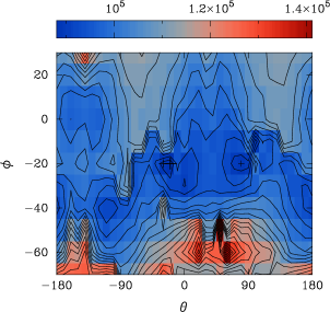
Figure 8: Left: Contours of the general multiparametric penalty function in $\theta,\phi$, with the largest plus symbol indicating the minimal value, and the other symbols indicating the next two best values. As for the binary envelope fit, the best fit cone solutions are seen to exist in two degenerate islands. Right: the various fit parameters, defined in §3, of the multiparametric model as a function of the penalty. The exponents $\gamma,\delta$ and $\nu$ are dimensionless, $\alpha_{c}$ is in degrees, and velocity scale $v_{0}$ and escape velocity $v_{e}$ are in $\rm cm\,s^{-1}$. All of the parameters tend to converge at the fit optimum, with the two islands of solutions giving similar values.

Fig. 9 shows the appearance of fine-tuned solutions, starting the optimizer in the two solution islands. The two solutions at $\theta_{A2}=-11^{\circ}$ and $79^{\circ}$ appear similar. Both attempt to account for the N and SE diffuse features, placing some dust in an approximately correct location, though with large residuals. The models underestimate the dust at the bottom of the envelope, in particular the lower “striae” of Fig. 2. Such features are almost certainly not in agreement with the simple powerlaw assumptions. Though these models account for the overall geometry, complex substructures are beyond their scope.

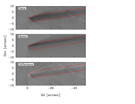
Figure 9: Left: Images of a fine-tuned solution at the left solution island of Fig. 8, converging to $\theta_{A2}=-11^{\circ},\phi_{A2}=-22^{\circ},\alpha_{A2}=45^{\circ}$. Right: Images of the the solution with the solver started at the right island, converging to $\theta_{A2}=79^{\circ},\phi_{A2}=-17^{\circ},\alpha_{A2}=45^{\circ}$. In each case, the original HST image is in the top panel, the model is in the middle, and the image minus the model is in the bottom. The envelopes from the previous section are over-plotted for reference only. Unlike the binary fit, this fit incorporates the faint diffuse features (Fig. 2), accounting for the higher maximum velocity of $v_{0}\sim 100\,\rm cm\,s^{-1}$.

In summary, our second fitting approach considered a model with powerlaw dependancies on dust size and velocity. We recovered approximately the same two islands of $\alpha_{c}=45^{\circ}$ solutions as the simpler binary fit method, this time at $\theta_{A2}=-11^{\circ},\phi_{A2}=-22$ and at $\theta_{A2}=79^{\circ},\phi_{A2}=-17^{\circ}$. These are again separated by about $90^{\circ}$ on the sky and differ by a rotation of one full cone width. We recover the previously obtained $\sim a^{-3.5}$ dust distribution, but the distribution in velocity is flatter than expected from cratering theory, with more dust at high velocities. The higher limiting debris velocity of the powerlaw fit arises from a filling of the N and SE diffuse features in Fig. 2.

4 Interpretation of the arc features

4.1 Description of features

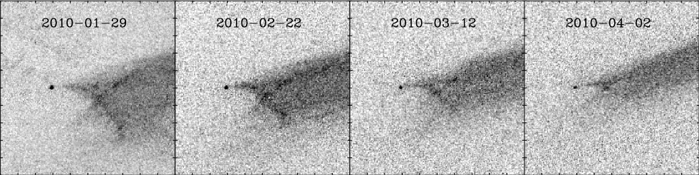
Figure 10: HST images of P/2010 A2, north up and east left, showing the evolution of the central debris feature with time. Each image is $10\arcsec\times 10\arcsec$, and each tick mark is $1\arcsec$. Most notable is the cross composed of a streak extending southwest from the nucleus, intersected by another streak extending to the northeast, denoted as Arcs 1 and 2 in Fig. 2.

To the west of the nucleus, there is a distinctive feature consisting of what appears to be two crossed trails or arcs (Fig. 2), about $10\arcsec$ in size; it is most visible in the early HST images of Jan and Feb 2010, and traces of it remain in later months (Fig. 10). Unless noted, we will focus on the feature as it appears on 29 Jan, when it was clearly traceable. Arc 2 points at the nucleus to its NE, but Arc 1 does not contact the nucleus at all, even if extended. Both features are within the dust envelope employed in the dust models, although Arc 2, the feature that points downward, is close to the left boundary of the envelope.

Additionally, there are other features like the striae along the tail direction, as noted in Fig. 2; these probably arise from secondary dust emission by debris. These features are beyond the scope of our models because there is no simple way to parameterize them. Indeed, these features involve time dependent processes, whereas our models all assume instantaneous ejection.

4.2 Possible distributions of debris emission

To interpret these arc–shaped, features, we will attempt to use general arguments of their dimensionality in physical space to constrain the particle size and the initial directional and velocity distribution of the debris.

Assuming a single time of outburst, any distribution of particles in space arises from a mapping of emission direction and velocity to three and two dimensional distributions $F_{3D}$ and $F_{2D}$ of the form (with the arrow “$\longrightarrow$” indicating a mapping from one space to another):

$$f(\theta_{A2},\phi_{A2},v_{\rm d},\beta)\longrightarrow F_{3D}(x,y,z)\longrightarrow F_{2D}(X,Y)$$ (2)

where $x,y,z$ are three dimensional spatial coordinates, and $X,Y$ are projected sky coordinates. In general, an $n$–dimensional manifold in $\theta_{A2},\phi_{A2},v_{\rm d},\beta$ emission-space will map to an $n-$dimensional manifold in $x,y,z$ or projected $X,Y$ physical space. For example, a two–dimensional surface in emission–space is described by two internal parameters, and it will continue to be described by these two parameters when emission–space is mapped to $x,y,z$ physical space. In order for $F_{2D}(X,Y)$ to be a one–dimensional curve, $F_{3D}(x,y,z)$ must be a one–dimensional curve or a two–dimensional sheet, and the same must be true of $f(\theta_{A2},\phi_{A2},v_{\rm d},\beta)$.

We first consider the possibility of a range of dust sizes by a simple numerical experiment: we launch particles at a fine grid in $\theta_{A2},\phi_{A2},v_{\rm d}$ in pairs of $\beta=0$ and $\beta=10^{-5}$. We trace the angular separation of the two valus of $\beta$ in each pair to determine the dust trail direction for that launch vector. We find that the position angle on the sky is always in a $3^{\circ}$ range around $278^{\circ}$, like the main trail. Hence there is no configuration of particles that could explain the cross-feature as a consequence of radiation–pressure driven trailing, because the position angle of both features is far from $278^{\circ}$. Hence the features must consist of a single particle size, and the only natural size is very large particles with $\beta=0$.

Noting that the arcs appear to be one–dimensional curves, there are two possibilities for the initial emission. First, the emission may be a one–dimensional curve in the space of $\theta_{A2},\phi_{A2},v_{\rm d}$. Examples might be a burst of debris in one direction $\theta_{A2},\phi_{A2}$ over a range of velocities, or emission over a curve in $\theta_{A2},\phi_{A2}$ at a single velocity. Second, the emission could be a two–dimensional surface in $\theta_{A2},\phi_{A2},v_{\rm d}$, mapping onto a surface in $x,y,z$ that is projected into a thin curve in $X,Y$. Examples of this second case might be a fan–like eruption, or one region of a hollow conical eruption.

4.3 Orbit models of the features

Having argued that the arcs consist of very large particles with $\beta=0$, and that the emission is either a one–dimensional curve or a two–dimensional surface in the emission space $\theta_{A2},\phi_{A2},v_{\rm d}$, we next attempt to determine which directions of emission could account for the feature. We integrate a library of particle orbits starting on 10 Feb 2009 and ending on 29 Jan 2010, each orbit defined by its launch direction $\phi_{A2},\theta_{A2}$ and its velocity $v_{d}$. In Figure 11 we show which of these orbits could account for the two arc components. Specifically, at a particular $v_{d}$, we color those regions of emission $\theta_{A2},\phi_{A2}$ that could populate each feature (shown in $X={\rm RA},Y={\rm Dec}$ sky space as an inset). By stacking these $\theta_{A2},\phi_{A2}$ slices in $v_{d}$, one can imagine a colored surface defined on a cube of $\theta_{A2},\phi_{A2},v_{\rm d}$. Emission must occur on a curve or sub–surface on this surface in order to fall onto the features.

Figure 11 immediately shows that the two sets of degenerate orbital features (blue and red colored islands) correspond in some way to the two degenerate dust cones that we derived previously, using either the binary or multiparametric fitting method (Fig. 6 and 8). Apparently, the viewing geometry is unable to distinguish between two equally good emission directions, but these two directions do not differ in their physical implications.

It is evident that there exists a debris velocity $v_{d}$ below which the features cannot be explained because the dust cannot reach the arc position. This is seen in those velocity slices (panes) of Fig. 11 where the $x,y$ inset picture of the feature is left black rather than red, blue, or green, meaning no orbits at that velocity fall on the feature. For Arc 1 in the top four–pane panel of Fig. 11, the $8.3\,\rm cm\,s^{-1}$ slice is ruled out, and for Arc 2 in the bottom panel, the $14.5\,\rm cm\,s^{-1}$ slice is excluded. After this minimum velocity is surpassed, the feature can be explained only with a rather complicated curve in the $\phi_{A2},\theta_{A2}$ plane. However, at larger velocities, the colored orbits split into two islands on the $\phi_{A2},\theta_{A2}$ plane, each of which suffices alone to explain the feature, again reflecting the existence of two solutions.

From the first part of Figure 11, Arc 1 can be explained by orbits that lie on the edge of the two degenerate dust cone solutions (dotted curves) that were fit previously. The velocities that work are 20 to 30 $\rm cm\,s^{-1}$, consistent with the dust cone fit. Because only orbits in a particular velocity range lie directly on the cones, it appears likely that the feature is localized in velocity if indeed it is part of the main cone. Encouragingly, this feature was not a part of the dust envelope used in the dust fit - hence the coincidence of the orbits with the outline of the dust cone is completely independent of the dust trail fit.

We then address the question of why this particular set of directions on the dust cone appear as a discrete feature. Figure 12 shows which emission directions were subject to greatest foreshortening (and thus visual enhancement) on 29 Jan 2010. To make this figure, pairs of particles separated by a $2\,\rm cm\,s^{-1}$ difference in velocity were launched in each direction at $v_{d}=28$ and $30\,\rm cm\,s^{-1}$, and the final separation on the sky within each pair was plotted as a grayscale image. Dark regions correspond to emission directions that are maximally foreshortened. It is apparent that the parts of the dust cone (red dotted line) that correspond to the first cross feature are among those that are most parallel to the line of sight. Thus the picture that suggests itself is that Arc 1 is a line of sight projection of large particles within a narrow velocity range on the best fit dust cone. An important caveat with Figure 12 is that it addresses only projection arising from a velocity spread. Other types of projection may also contribute, like the edge brightening of a hollow cone viewed from the side.

The orbits explaining Arc 2, in the second panel of Figure 11, also touch the best–fit dust envelope cone, like Arc 1. However, these orbits do not fit the cone as well as those of Arc 1, though the highlighted arc of orbits does agree strikingly well with the most foreshortened regions in Figure 12. Hence it is likely that Arc 2 represents extended debris from main cone that also happens to fall into the directions of maximum line–of–sight projection.

When Fig. 12 is recomputed using the features as observed on 12 March 2010 and 2 April 2010 (see Fig. 10), using the analogous but highly evolved features on these dates, the figure resembles the original 29 Jan 2010 version, demonstrating that the orbital interpretation remains consistent with time.

It is also possible to show that both Arcs 1 and 2 may be fully recreated using only those orbits lying precisely on either of the cones, by selecting orbits on particular curves in the space of velocity and the cone’s azimuthal parameter. Given the freedom to place arbitrary curves of overdensity on the depicted cones, one can easily recreate the features. However, different cones work as well, and such ad hoc curves have no obvious physical interpretation beyond arising from inherent asymmetries in the ejection event.

In summary, our procedure of mapping out which large–particle debris orbits could account for the Arcs 1 and 2 shows that the allowed initial trajectories constitute a surface in emission space, as surmised in Sec. 4.2. Moreover, the trajectories largely coincide with the previously determined best–fit dust cone. For the case of Arc 1 at least, the permitted orbits are completely independent of the data that went into the fitting of the dust cone, so there are two separate pieces of evidence pointing at conical emission in the directions computed.

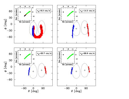
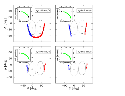
Figure 11: A depiction of which large particle ($\beta=0$) initial debris orbits emitted on 2009 Feb 10 and ending on 2010 Jan 29 could have accounted for the Arc 1 (top panel) and Arc 2 (bottom panel) features (see Fig. 2). The separate four–panel plots show the two components of the cross individually, depicted on the RA, Dec plane within the inset. Within each plot, each of the four panels represents one initial particle velocity, and the axes $\phi_{A2},\theta_{A2}$ are the emission direction of the debris. Colored regions in the $\phi_{A2},\theta_{A2}$ plane are debris orbits that fall onto the observed feature; they are coded blue and red to denote the two separate islands of solutions on the $\phi_{A2},\theta_{A2}$ plane. In the RA, Dec inset showing the feature on the sky, regions of the feature are colored red and blue if they are explained by the corresponding orbits in the larger $\phi_{A2},\theta_{A2}$ plot, green if both the red and green solutions can explain them, and black if no particle orbits can explain this part of the feature. The $+$ symbols and the dotted curves around it are the two solutions best fit dust cones from the first part of the modeling (Fig. 6 and 8 ). As discussed in the text, there is considerably overlap between the edges of the best fit dust cone and the discrete features in the insets. There is also a correspondence of the features with the regions of maximum foreshortening shown in Figure 12.

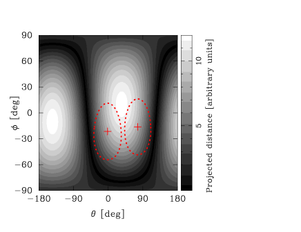
Figure 12: A depiction of the foreshortening of debris orbits emitted on 2009 Feb 10 and ending at 2010 Jan 29, with the emission occurring in the direction $\phi_{A2},\theta_{A2}$ and a velocity $v_{d}=31\,\rm cm\,s^{-1}$. Dark regions indicate directions in which particles emitted at slightly different velocities remain close on the sky, and light regions are where such particles appear more separated. Strings of debris emitted in directions where the figure is dark will be less dispersed and more visible. The red $+$ symbols and the dotted curve around it are the nearly degenerate best fit dust cone solutions from the first part of the modeling. The right side ($\theta_{A2}\approx 110^{\circ}$) of the the right cone or the left side of the left cone should have enhanced visibility, and, indeed, these regions correspond to the two solutions for Arc 1 and 2 in Fig. 11. In particular, the orbits that could account for Arc 2 exist exclusively in the darkest regions of this figure.

4.4 A simple model of P/2010 A2

Figure 13 illustrates a very simple model based on some of the inferences we have described. The principal feature of this model is a $\beta=0$ dust cone at $\phi_{A2}=-20^{\circ},\theta_{A2}=74^{\circ}$, with ${v_{\rm d}}_{\rm max}=35\,\rm cm\,s^{-1}$. It is consistent with the dust envelope models. The cone has an additional feature in the form of an overdensity in velocity space from 14 to $22\,\rm cms^{-1}$, producing an elliptical band that, in projection, resembles Arc 1. The bottom edge of the cone, made brighter by projection, resembles Arc 2. The cone opening angle increases with velocity from $33^{\circ}$ to $40^{\circ}$ to produce the curvature observed in the second feature; this will be discussed below.

We emphasize that this is not a best–fit model, but merely a representation of the outburst that agrees with our previous fits of the dust envelope and inferences about the arcs. A notable oversimplification is that we assume the ejecta to be symmetric around the central axis, which is certainly unjustified for a glancing impact. Such non–uniformity may explain why only parts of the ring feature are visible, and why the brightest part is not the part viewed in strongest projection. We also assume no gravity; when gravity corresponding to a massive P/2010 A2 variant, modeled as a sphere $100\,\rm m$ in radius with density $3500\,\rm kg\,m^{-3}$ is introduced, the entire debris ensemble is pulled to the left by about an arcsecond, arguing against such a massive body. Less massive variants of the nucleus, like those considered in Paper I, do not exhibit this shift. Another shortcoming of this simple model is that the arc features touch but do not fully cross, unlike the actual data. This can be ameliorated by making the opening angle of the debris ring larger than that of the cone, but there is no obvious physical reason to do this.

A final limitation of this simple model is the fact that there is a consensus that impact debris cones tend to widen at lower velocities (Richardson et al. 2007), whereas our cone is made narrower to make it agree with the observed curvature of the debris feature. However, some laboratory studies (Anderson et al. 2003; Cintala et al. 1999) find that the cone re–narrows at the final low–velocity stage of excavation, which is the regime relevant to the visible debris.

When we continue the integration to the 2010 March, April, and May dates of the later HST images of Jewitt et al. (2010b), then the development of our model subjectively matches that of P/2010 A2, with the features becoming narrower and trailing further behind the nucleus.

Despite its ad hoc nature, this model shows that much of the observed structure can be roughly replicated using only the best-fit cone of the overall dust envelope, with the addition of non-uniformity in velocity and a velocity variation in opening angle. Unfortunately, a full fit of a cone plus ring model would be extremely difficult: it would require optimizing over at least six parameters, would not account for asymmetries (e.g. local terrain), would be contaminated with $\beta>0$ dust, and would not have any obviously correct merit function for the fit.

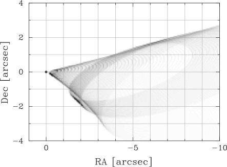
Figure 13: Left: A toy model of $\beta=0$ debris ejection at $\phi_{A2}=-20^{\circ},\theta_{A2}=74^{\circ}$. An excess of ejecta at a velocity of $14$ to $22\,\rm cm\,s^{-1}$ has been used to create the elliptical band inside the cone, resembling one of the features of the data. To illustrate a mechanism by which the oberved curvature might be produced, the cone tapers from a width of $\alpha_{c}=40^{\circ}$ at its outer extreme velocity of $35,\rm cm\,s^{-1}$ to a width of $\alpha_{c}=33^{\circ}$ at its inner velocity of $0\,\rm cm\,s^{-1}$. . The boundaries of the cone are brightened by edge effects, and correspond very roughly to the other main feature of the data. Right: the 29 Jan 2010 HST image, for comparison. The model for the second (degenerate) solution at $\theta_{A2}\approx-5^{\circ}$ appears similar.

4.5 Physical implications of ejecta geometry

Cratering phenomena and ejecta distributions have been studied extensively using scaling laws based on dimensional arguments, hydrodynamic simulations, and laboratory experiments (e.g. R2007, and Holsapple (1993)). Our finding of a $\alpha_{c}\approx 45^{\circ}$ hollow cone is in broad agreement with a number of sources cited in R2007, which find ejection angles $\psi=90^{\circ}-\alpha_{c}$ ranging from $35^{\circ}$ to $63^{\circ}$, corresponding to $\alpha_{c}=55^{\circ}$ to $27^{\circ}$. In laboratory experiments involving the impact of high–speed projectiles into sand, the most common value appears to be $\psi\approx 50^{\circ}$, in agreement with our value $\alpha_{c}\approx 40^{\circ}$ (Anderson et al. 2003; Cintala et al. 1999).

Henceforth, we will use the R2007 formulation of cratering to discuss some interpretations of our modeling of the observed phenomena. We strongly emphasize, however, that many aspects of cratering, particularly late–stage effects, are poorly understood, and that our conclusions hinge on the uncertain validity of these models. The standard cratering formulation of R2007 is almost certainly an oversimplification that is at odds with experiment. Nevertheless, we believe that the arguments are at least qualitatively valid, and provide physical motivation for aspects of the simple model in the previous section.

Jewitt et al. (2010b) assume a mm to cm range of particle sizes and find that the visible ejecta correspond to a sphere having a volume $V_{\rm ej}\in[2\times 10^{4},2\times 10^{5}]\,\rm m^{3}$, so that the radius $R_{c}$ of the crater is $R_{c}\approx{V_{e}}^{1/3}\sim 30$ to $\sim 60\,\rm m$ from Equation 11 of R2007. Similarly, in Paper I, we measure particles spanning diameters of 1 to 20 mm, and a slightly larger volume of ejecta of $2.7\times 10^{5}\,{\rm m^{3}}$, also giving a crater with $R_{c}\sim 60\,{\rm m}$.

The accuracy of the volume estimate varies linearly with the accuracy of the estimated debris particle size, so the accuracy of the crater radius $R_{c}$ is much better, going as the $\frac{1}{3}$ power of the particle size, which will be useful below.

In the simplified model of cratering, the crater radius $r_{c}$ grows in a outflow of material, and debris is emitted at a velocity $v_{e}\propto{r_{c}}^{-\frac{1}{\mu}}$, with $\mu\in[0.41,0.55]$, until a strength–limited or gravity–limited crater volume and radius are reached (Equations 13 and 37 in R2007). The first panel of Fig. 14 illustrates this for a model of P/2010 A2 resembling our estimate in Paper I: the radius of the target is $85\,\rm m$, the density is $3000\,{\rm kg\,m^{-3}}$, and the $r_{i}=0.6\,\rm m$ impactor, having the same density, strikes at $v_{i}=3\,{\rm km\,s^{-1}}$. The impactor is made slightly smaller and slower than our canonical values of $r_{i}=1\,\rm m$ and $v_{i}=5\,{\rm km\,s^{-1}}$ to give crater sizes on the order of the $60\,\rm m$ estimate, rather than being larger than P/2010 A2. In this figure, the ejection velocity (ordinate) falls with crater radius (abscissa), until the velocity plummets to zero at some critical strength-limited radius (dotted vertical lines) given by the strength $Y$, where the flow is no longer sufficiently energetic to break the material. At the lowest strengths, the crater radius never reaches strength–limited radius because gravity contributes to the truncation of growth. In both the strength–limited and gravity–limited regimes, the velocity curve has a sharp break or knee at the truncation radius. In both regimes, the maximum amount of debris is ejected just before the crater’s limiting radius, by considering the area of the crater at the moment of truncation.

The $v_{e}(r)$ curve plotted in the left panel of Fig. 14 may be numerically inverted to give $r(v_{e})$, and the amount of mass ejected at a particular velocity may then be written as $dM/dv_{e}\propto dM/dr\,\,dv_{e}/dr\propto r^{2}(v_{e})\,dv_{e}/dr$. The sharp bend in $v_{e}(r)$ gives a large value for the derivative $dv_{e}/dr$, which, combined with the large value of ${r_{e}}^{2}$, produce a peak in debris at low velocities. This peak is shown in the right panel of Fig. 14: $Y\sim 0.5\,\rm kPa$ produces peaks in the debris around the value of $14\,\rm cm\,s^{-1}$ that we attribute to Arc 1, and also gives a crater of an appropriate size. The system is generally

This low strength corresponds to a loose powdery surface, comparable to lunar soil ($Y\sim 1\,\rm kPa$, Mitchell et al. (1972)) and snow ($Y\sim 0.5\,\rm kPa$, Sommerfeld (1974)). A caveat is the fact that the concept of material strength in impacts is not well defined, so the $Y$ given is a formal value with an uncertain physical interpretation. This entire approach should be viewed with caution, because the cratering physics is greatly oversimplified, and because the parameters of the system, though chosen from within the the range indicated by observations, were tuned to give the desired velocity peak and crater size. Nevertheless, Fig. 14 suggests that high material strengths will not produce a peak of material at a low velocity, but low strengths can be made qualitatively consistent with the physical picture that emerges from orbit modeling.

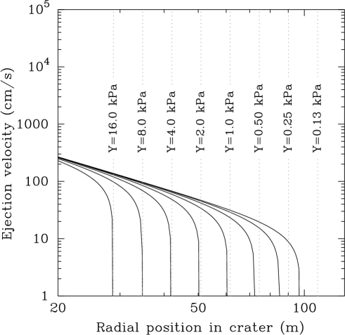
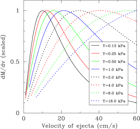
Figure 14: Left: Right: the ejection velocity (not corrected for $v_{e}$) as a function of the radial position in the crater, with a terminus at the strength–limited crater radius (dotted lines at each strength $Y$). Each solid curve corresponds to one value of $Y$. We used an $85\,\rm m$ target radius, an $3000\,\rm kg\,m^{-3}$ target density, and a $0.7\,\rm m$ impactor moving at $3\,\rm km\,s^{-1}$, close to the nominal values from Paper I. Note that for small $Y$ crater growth stops before the corresponding dotted strength limit as gravity becomes relatively important at low strengths. Right: the differential distribution of ejected mass as a function of ejection velocity (corrected for $v_{e}$) for various target material strengths $Y$. Only the lower target strengths correspond to the low debris velocities observed.

Throughout, we have assumed a symmetric ejection event, corresponding to a vertical or near—vertical impact. In an oblique impact that is more than $60^{\circ}$ from the vertical, debris becomes preferentially distributed in the downrange direction, and a gap in the cone appears in the direction from which the impactor arrived (Pierazzo & Melosh 2000, and R2007). The features observed in Fig. 11 could be one side of an asymmetrical impact cone, implying that the impactor arrived from $\theta_{\rm A2}\sim 0^{\circ}$, outside P/2010 A2’s orbit. Because the features are close to the directions of maximum projection (Fig. 12), it is hard to distinguish between an oblique impact and a symmetric cone that is selectively enhanced by the viewing geometry, as in Fig. 13. Equations 44, 45, and 46 of R2007 provide an approximation to the modifications of the ejection angle and velocity resulting from an oblique impact, but these variations turn out to be much too small to be visible, and cannot account for the curvature of the second cross feature (Fig. 11, right).

In conclusion, it is very plausible that the ring–shaped feature (peak in the velocity distribution) suggested by the first panel of Fig. 12 and by Fig. 13 is in fact related to the expected peak in the debris velocity distribution: it may be the last, slowest, and most abundant debris before the cratering process halted. In this respect, it differs from the Tempel 1 Deep Impact result (Holsapple & Housen 2007, e.g.), where the tensile-strength limited velocity was apparently below the escape speed, and the plume never detached. A further argument for plume detachment in the P/2010 A2 data is the visible gap separating the nucleus and debris trail (HST image, Fig. 13)

5 Summary and discussion

The peculiar collection of debris surrounding P/2010 A2 has several possible explanations. As originally pointed out by Jewitt et al. (2010b), it may arise from disruption after rotational spin–up, from prolonged sublimation activity, or from a collision, the hypothesis examined in this paper. We found broad agreement with a conical ejection event, and the large particles argue against sublimation, but we did not specifically find disagreement with a spin–driven disruption. To confirm or rule out this last possibility, similar orbit modeling could be applied to the ejecta distributions produced by spin–disruption. Naively, a $200\,\rm m$ body spinning at the shortest 2.1 hour period permitted for a non–cohesive rubble pile would have a surface speed of $8\,{\rm cm\,s^{-1}}$, far less than the observed debris velocity of $\sim 30\,{\rm cm\,s^{-1}}$. However, a faster cohesive body cannot be ruled out (Holsapple 2007).

In this paper, we examined whether the January 2010 trail behind P/2010 A2could be explained with a conical ejecta distribution from an impact event. Specifically:

1. We performed fit (§2) using binary filling of a drawn-by-eye dust envelope, finding that two islands in the space of ejection direction yield $\alpha_{c}\sim 40^{\circ}$ half angle ejecta cones that fill the observed dust envelope. A $\sim 40^{\circ}$ cone is in agreement with cratering theory and experiment. The two islands correspond to rotating the cone by one full width, so their $\sim 90^{\circ}$ separation is further evidence of the validity of the d $\alpha_{c}\sim 40^{\circ}$ cone solution – i.e there is something in the system with a characteristic angular scale of $\sim 90^{\circ}$. The main narrow bright trail extending directly from the nucleus corresponds to a direction on the cone that is more aligned with the effect of solar pressure, resulting in coherent motion rather than solar pressure driven spreading.

2. We created a second set of models (§3), using power law distributions for the dust size, velocity, and velocity–cutoff, and employing an absolute value deviation metric between the image and the model. We found that the same two ejection geometries provided the best fit, suggesting that this result is robust against the assumptions of the fitting method. These models gave a dust size exponent that matched previous results, but gave an excess of dust at large velocities relative to cratering theory. They also placed higher velocity dust at the locations of the the N and SE diffuse features (Fig. 2).

3. We argue that the two bright arc features (Fig. 2) must consist of sheet–like or line–like ejection (§4). We integrated the trajectory of large ($\beta=0$) dust particles in all possible directions, to see which directions could plausibly land on the two bright arc features. We found that the orbits corresponding to the bright arcs are low velocity debris lying on the same $\alpha_{c}\approx 40^{\circ}$ cones found in the dust fits (Fig. 11), which did not use knowledge of the features. This agreement provides independent support for a $\alpha_{c}\approx 40^{\circ}$ ejection cone. We argue that one of the features is an edge–brightened region of cone enhanced by an alignment of the line of sight with the local velocity vector, and the other may be a concentration of debris in velocity. The features thus result from debris coincident with the cone, viewed in projection. We construct a simple model using these ideas that qualitatively reproduces some of the salient features of P/2010 A2.

4. We apply standard cratering theory to argue that a peak quantity of debris at a low non–zero velocity is a natural consequence of an impact. If the second arc feature corresponds to such a peak in the velocity distribution, it is agreement with an impact into loose regolith.

We argue that from several different perspectives, a consistent view of P/2010 A2’s activity emerges: it is probably the result of a single impact into a loose surface, throwing debris outward in a well–known hollow $\sim 40^{\circ}$ half-opening angle conical pattern, in qualitative agreement with theoretical and laboratory studies of impact cratering. Further work will require addressing asymmetries in the impact, and more complicated velocity distributions. Such improvements may be constrained by the limited available data, which are contaminated by artifacts, and by the unknown effects of the target’s terrain and topography.