Geometric Momentum as a Probe of Embedding Effect

Abstract

As a submanifold is embedded into higher dimensional flat space, quantum mechanics gives various embedding quantities. In the present study, two embedding quantities for a two-dimensional curved surface examined in three-dimensional flat space, the geometric momentum and the geometric potential, are derived in a unified manner. Then for a particle moving on a two-dimensional sphere or a free rotation of a spherical top, the projections of the geometric momentum $\mathbf{p}$ and the angular momentum $\mathbf{L}$ onto a certain Cartesian axis form a complete set of commuting observables as $[p_{i},L_{i}]=0$ ($i=1,2,3$), thus constituting a dynamical ($p_{i},L_{i}$) representation for the states on the two-dimensional spherical surface. The geometric momentum distribution of the state represented by spherical harmonics is successfully obtained, and this distribution for a homonuclear diatomic molecule seems within the resolution power of present momentum spectrometer and can be measured to probe the embedding effect.

I Introduction

In microscopic domain, there are many quantum motions confined on the two-dimensional surfaces, e.g., mobile carriers on the corrugating graphene sheet or spherical fullerene molecule $C_{60}$, and free rotation of hydrogen nuclei around its center of mass in a hydrogen molecule at relatively low temperature, etc. Over the past decade, we have witnessed that physics community gradually reaches consensus that the examination of the quantum motions confined on the two-dimensional surfaces in three-dimensional Euclidean space $R^{3}$ is of physical significance. In the Euclidean space, the quantum physics is well defined, one can use conventional quantum mechanics without any new postulate imposed dirac1 ; dirac2 . The confinement of the particle on a curved two-dimensional manifold is treated as the limiting case of a particle in a three-dimensional manifold in which a confining potential is invoked to acting in the normal direction of its two-dimensional surface, and we can then have an unambiguous formulation of quantum mechanics on the surface as a secondary or derived theory jk ; dacosta ; 1992 ; kleinert ; 1997-1 ; 1998 ; FC ; JD ; OB ; liu11-1 ; SOint1 ; SOint2 ; SOint3 ; SOint4 ; 2010-2 ; epl . However, if one hopes to reproduce the same theory within the Dirac’s theory for a systems with second class constraints dirac2 , some cautions need to be taken into consideration note0 . The new formulation of quantum mechanics on the surface involves both gaussian and mean curvature. In simple and plain words, the mean curvature $M$, on one hand, is an extrinsic curvature that is not detectable to someone who can not study the three-dimensional space surrounding the surface on which he resides, whereas the gaussian curvature $K$, on the other hand, is an intrinsic curvature that is detectable to the “two-dimensional inhabitants” on a surface and not just outside observers wolfram . In purely intrinsic geometry, undefinable and even meaningless is the shape itself of a surface.

When no electromagnetic field is applied and the spin of the particle plays insignificant role, the marked feature of the theory is the dependence of both an effective potential $V_{g}$ note1 in the Hamiltonian and the geometric momentum $\mathbf{p}$ on the mean curvature $M$ jk ; dacosta ; FC ; JD ; OB ; liu11-1 . The geometric potential jk ; dacosta ; note1 with $\mu$ denoting the mass,

$$V_{g}=-\hbar^{2}/(2\mu)(M^{2}-K)$$ (1)

comes from how to define a proper form of Laplacian operator acting on a quantum state on surface liu11-1 ; 2007 , whereas the geometric momentum, with $\mathbf{\nabla}_{2}$ being the gradient operator on a two-dimensional surface diffgeom and $\mathbf{n}$ standing for the normal vector of the surface at a given point,

$$\mathbf{p}=-i\hbar(\mathbf{\nabla}_{2}+M\mathbf{n}),$$ (2)

is related to a proper form of gradient operator on the state liu11-1 . When first exposed to this expression (2) apparently containing a term $M\mathbf{n}$, many thinks it has component along the normal direction, but it is not the case. Actually, it is an operator exclusively defined on the tangent plane to surface at the given point for we have an operator relation $\mathbf{p}\cdot\mathbf{n+n}\cdot\mathbf{p}=0$ with use of a relation$\ \nabla_{2}\cdot\mathbf{n}=-2M$ diffgeom . One can also call (1) and (2) the embedding potential japan1993 and the embedding momentum, respectively. As we see in the appendix, both geometric quantities (1) and (2) can be derived within the same theoretical framework. An experimental verification of the potential amounts to an indirect affirmative experimental evidence of the momentum as well, and vice versa. The geometric potential has recently been experimentally verified 2010-2 ; epl , and it is an important advance in quantum mechanics, implying that quantum mechanics based on purely intrinsic geometry does not offer a proper description of the constrained motions in microscopic domain, provided that the extrinsic examination is performed as well. Here we mention that the spin of the particle usually plays a role via the surface spin-orbit coupling SOint1 ; SOint2 ; SOint3 , etc.SOint4 , obtained also from the same procedure of squeezed limit of its the three-dimensional analogue.

Noting that the linear momentum distribution of an electron state within a hydrogen atom can be easily carried out and had been experimentally verified MomentumSpect1 ; MomentumSpect2 . Let us consider the simplest constrained motion on two dimensional spherical surface $S^{2}$ and ask whether it is possible to give a momentum space representation for the states on it. An immediate problem is what the proper momentum is. It can never be the usual linear momentum $-i\hbar\mathbf{\nabla=}-i\hbar\mathbf{(\partial}_{x},\mathbf{\partial}_{y},\mathbf{\partial}_{z}\mathbf{)}$ because the motion on $S^{2}$ has only two degrees of freedom while $-i\hbar\mathbf{\nabla}$ has three mutually commutable components that are too many to form a complete set of commuting observables for $S^{2}$. Moreover, as we stress before liu11-1 , a set of self-adjoint momentum operators in purely intrinsic geometry is unattainable for any states on $S^{2}$. In addition, the geometric momentum $\mathbf{p}=-i\hbar(\mathbf{\nabla}_{2}+M\mathbf{n})$ (2) alone does not suffice because its three components are not mutually commutable, thus too few to provide a complete set of commuting observables. The key finding of the present study offers a solution to the problem, based on a discovery of a new dynamical representation on the surface.

The organization of the present paper is as follows. In next sections II, we present a unified derivation of both geometric potential (1) and momentum (2). In next sections III, we starts from a dynamical symmetric group $SO(3,1)$ on the sphere which yields a proper and complete set of commuting observables, to arrive at a dynamical representation mixing the geometric momentum and orbital angular momentum. In the section IV, it aims at the explicit form of the geometric momentum distribution of the some molecular rotational states. Section V gives a brief discussion of the results obtained, and conclude the present study.

II Geometric momentum for a particle on a curved surface

To get the geometric momentum (2), we utilize exactly the same manner how the geometric potential is derived jk ; dacosta ; FC . For ease of the comparison, we use similar set of symbols as Ferrari and Cuoghi who recently build up a theoretical framework with geometric potential when the electromagnetic field is applied FC . The lowercase Latin letters $i,j,k$ stand for the 3D indices and assume the values $1,2,3$, e.g., $\mathbf{(}x_{i},p_{j}\mathbf{)}$ for the position and momentum in 3D Cartesian coordinates. Position specified by ($q^{1},q^{2},q^{3}$) can be understood as description of the position in the curvilinear coordinates parameterizing a manifold. Now let the 2D surface under study is considered as a more realistic 3D shell whose equal thickness $d$ is negligible in comparison with the dimension of the whole system. The position $\mathbf{R}$ within the shell in the vicinity of the surface $S$ can be parametrized as with $0$ $\leq q^{3}\leq d,$

$$\mathbf{R}(q^{1},q^{2},q^{3})=\mathbf{r}(q^{1},q^{2})+q^{3}\mathbf{n}(q^{1},q^{2}),$$ (3)

where $\mathbf{r}(q^{1},q^{2})$ parametrizes the surface and $\mathbf{n}(q^{1},q^{2})$ denotes the unit normal vector at point $(q^{1},q^{2})$. The gradient operator $\nabla$ in 3D flat space, expressed in the curvilinear coordinates, takes following form diffgeom ,

$$\nabla=\mathbf{r}^{\mu}\partial_{\mu}+\mathbf{n}\partial_{q^{3}}\text{,}$$ (4)

where $\mathbf{\nabla}_{2}\equiv\mathbf{r}^{\mu}\partial_{\mu}$ is the gradient operator on 2D curved surface diffgeom . The relation between the 3D metric tensor $G_{ij}$ and the 2D one $g_{\mu\nu}$ is given by dacosta ; FC ,

$$G_{ij} =g_{\mu\nu}+\left[\alpha g+(\alpha g)^{T}\right]_{\mu\nu}q^{3}+(\alpha g\alpha^{T})_{\mu\nu}\left(q^{3}\right)^{2},$$

$$G_{\mu 3} =G_{3\mu}=0,\;G_{33}=1,$$ (5)

where $\alpha_{\mu\nu}$ is the Weingarten curvature matrix for the surface, and $M=-\mathrm{Tr}(\alpha)/2$, and $K=\mathrm{\det}(\alpha)$ dacosta . The covariant Schrödinger equation for particles moving within a thin shell of thickness $d$ in 3D is FC , with presence of both the magnetic field via the vector potential $\mathbf{A}$ and the electric field via the scalar potential $V$,

$$\mathrm{i}\hbar\frac{\partial}{\partial t}\psi(\mathbf{q},t)=-\frac{\hbar^{2}}{2m}G^{ij}D_{i}D_{j}\psi(\mathbf{q},t)+QV\psi(\mathbf{q},t),$$ (6)

where $Q$ is the charge of the particle and $D_{j}=\nabla_{j}-(\mathrm{i}Q/\hbar)A_{j}$ with $A_{j}$ being the covariant components of the vector potential $\mathbf{A}$. Conveniently denoting the scalar potential $A_{0}=-V$, we can define a gauge covariant derivative for the time variable as $D_{0}={\partial_{t}}-{\mathrm{i}Q}A_{0}/\hbar$. The gauge transformations in quantum mechanics are FC ,

$$A_{j}\rightarrow A_{j}^{\prime}=A_{j}+\partial_{j}\gamma;\text{ }A_{0}\rightarrow A_{0}^{\prime}=A_{0}+{\partial_{t}}\gamma;\text{ }\psi\rightarrow\psi^{\prime}=\psi\mathrm{e}^{\mathrm{i}Q\gamma/\hbar},$$ (7)

where $\gamma$ is a scalar function. The Eq.(6) can be rewritten as an explicit gauge invariant form FC ,

$$\mathrm{i}\hbar D_{0}\psi=-\frac{\hbar^{2}}{2m}G^{ij}D_{i}D_{j}\psi.$$ (8)

Now we recall two important facts regarding the wave functions: 1, the normalization of the wave functions remains whatever coordinates are used, and the transformation of volume element satisfies $d^{3}\mathbf{x=}\sqrt{G}d^{3}\mathbf{q}$ FC ,

$$\int\left|\psi(\mathbf{x},t)\right|^{2}\mathrm{d}^{3}\mathbf{x=}\int\left|\psi(\mathbf{q},t)\right|^{2}\sqrt{G}\mathrm{d}^{3}\mathbf{q}=1,$$ (9)

where dacosta ; FC ,

$$G=\mathrm{det}(G_{ij})=g\left(1-2Mq^{3}+K\left(q^{3}\right)^{2}\right)^{2}.$$ (10)

2, an advantage of the coordinates (3) is that the wave function $\psi(\mathbf{q},t)$ from (6) or (8) takes following factorization form dacosta ; FC ,

$$\psi(\mathbf{q},t)=\frac{\chi(q^{1},q^{2},t)}{\sqrt{1-2Mq^{3}+K\left(q^{3}\right)^{2}}}\varphi(q^{3},t),$$ (11)

and it is guaranteed with suitable choice of gauge for $\gamma$ such that $A_{3}^{\prime}=0$ FC ,

$$\gamma(q^{1},q^{2},q^{3})=-\int_{0}^{q^{3}}A_{3}(q^{1},q^{2},q)\mathrm{d}q.$$ (12)

Combining these two facts, we have two conservations of norm from (9),

$$\oint\left|\chi(q^{1},q^{2},t)\right|^{2}\sqrt{g}\mathrm{d}q^{1}\mathrm{d}q^{2}=1,\text{ and }\int_{0}^{d}\left|\varphi(q^{3},t)\right|^{2}\mathrm{d}q^{3}=1.$$ (13)

We are now ready to examine the gradient operator $\nabla$ (4) acting on the state $\psi(\mathbf{q},t)$ and the result is,

$$\nabla\psi(\mathbf{q},t) =\mathbf{r}^{\mu}\partial_{\mu}\psi(\mathbf{q},t)+\mathbf{n}\frac{M-q^{3}K}{\left(1-2Mq^{3}+K\left(q^{3}\right)^{2}\right)^{3/2}}\chi(q^{1},q^{2},t)\varphi(q^{3},t)$$

$$+\mathbf{n}\frac{\chi(q^{1},q^{2},t)}{\sqrt{1-2Mq^{3}+K\left(q^{3}\right)^{2}}}\partial_{q^{3}}\varphi(q^{3},t).$$ (14)

Then taking limit $d\rightarrow 0$, we have $\nabla$ as its acting on the state $\psi(\mathbf{q},t)$,

$$\nabla\psi(\mathbf{q},t)=\left(\mathbf{r}^{\mu}\partial_{\mu}+M\mathbf{n}\right)\psi(\mathbf{q},t)+\mathbf{n}\chi(q^{1},q^{2},t)\partial_{q^{3}}\varphi(q^{3},t)$$

which shows that the gradient operator $\nabla$ can be decomposed into two separate parts, one part $\left(\mathbf{r}^{\mu}\partial_{\mu}+M\mathbf{n}\right)$ lies on the tangent plane to surface at a given point and another is along the direction of normal $\mathbf{n}$, corresponding to the decomposition of the Schrödinger equation into two Schrödinger ones determining $\chi(q^{1},q^{2},t)$ and $\varphi(q^{3},t)$ respectively FC . Paying attention to the motion on the surface only, we have the resultant operator, $\mathbf{r}^{\mu}\partial_{\mu}+M\mathbf{n}$. With a coefficient $-i\hbar$ multiplied, the geometric momentum (2) is derived.

The gauge invariance of the momentum operator $\mathbf{p}=-i\hbar(\mathbf{r}^{\mu}\partial_{\mu}+M\mathbf{n)-}Q\mathbf{A}$ is assured in the presence of the vector potential $\mathbf{A}$ with vanishing component along the normal direction as $A_{3}=0$ being pre-imposed. Under 2D gauge transformation: $\mathbf{A}\rightarrow\mathbf{A}^{\prime}=\mathbf{A+r}^{\mu}\partial_{\mu}\gamma$ with $\gamma=\gamma(q^{1},q^{2})$ and $\psi\rightarrow\psi^{\prime}=\mathrm{e}^{\mathrm{i}Q\gamma/\hbar}\psi$, we have $\mathbf{p}\psi\rightarrow\mathbf{p}^{\prime}\psi^{\prime}=\mathrm{e}^{\mathrm{i}Q\gamma/\hbar}\mathbf{p}\psi$,

$$\mathbf{p}^{\prime}\psi^{\prime} =\left(-i\hbar(\mathbf{r}^{\mu}\partial_{\mu}+M\mathbf{n)-}Q(\mathbf{A}+\mathbf{r}^{\mu}\partial_{\mu}\gamma)\right)\psi\mathrm{e}^{\mathrm{i}Q\gamma/\hbar}$$

$$=\mathrm{e}^{\mathrm{i}Q\gamma/\hbar}\left(-i\hbar(\mathbf{r}^{\mu}\partial_{\mu}+M\mathbf{n)-}Q\mathbf{A}\right)\psi$$

$$=\mathrm{e}^{\mathrm{i}Q\gamma/\hbar}\mathbf{p}\psi.$$ (15)

Noting that there is no direct connection between $\Delta_{LB}+(M^{2}-K)$ and $\nabla_{2}+M\mathbf{n}$ such as in 3D flat space $\nabla^{2}\equiv\nabla\cdot\nabla$. For reaching $\Delta_{LB}+(M^{2}-K)$, we have to start from the Laplace operator in flat 3D space$\ \nabla^{2}=\left(\mathbf{r}^{\mu}\partial_{\mu}+\mathbf{n}\partial_{q^{3}}\right)\cdot\left(\mathbf{r}^{\mu}\partial_{\mu}+\mathbf{n}\partial_{q^{3}}\right)=\Delta_{LB}-2M\partial_{q^{3}}+\partial_{q^{3}}^{2}$ diffgeom , then resort to the confining procedure. Explicitly we have,

$$\nabla^{2}\psi(\mathbf{q},t) =\Delta_{LB}\psi(\mathbf{q},t)+\frac{(M^{2}-K)+2M(2M^{2}-K)q^{3}+2K(K-3M^{2})\left(q^{3}\right)^{2}+2MK^{2}\left(q^{3}\right)^{3}}{\left(1-2Mq^{3}+K\left(q^{3}\right)^{2}\right)^{5/2}}\psi(\mathbf{q},t)$$

$$-\frac{2q^{3}(K-2M^{2}+KMq^{3})}{\left(1-2Mq^{3}+K\left(q^{3}\right)^{2}\right)^{3/2}}\chi(q^{1},q^{2},t)\partial_{q^{3}}\varphi(q^{3},t)+\frac{1}{\left(1-2Mq^{3}+K\left(q^{3}\right)^{2}\right)^{1/2}}\chi(q^{1},q^{2},t)\partial_{q^{3}}^{2}\varphi(q^{3},t)$$ (16)

In the same limit limit $d\rightarrow 0$, this operator $\nabla^{2}$ (16) becomes,

$$\nabla^{2}=\Delta_{LB}+(M^{2}-K)+\partial_{q^{3}}^{2}$$ (17)

Noting that kinetic energy is $T=-\hbar^{2}/(2\mu)\nabla^{2}$, we see that the effective potential, the geometric potential as $-\hbar^{2}/(2\mu)(M^{2}-K)$ (1) comes out. However, it is a puzzling fact that there is a direct connection between $\left(\mathbf{r}^{\mu}\partial_{\mu}+M\mathbf{n}\right)$ and$\ \Delta_{LB}$ 2007 , as we pointed out in 2007. What puzzling? the quantity $\left(\mathbf{r}^{\mu}\partial_{\mu}+M\mathbf{n}\right)$ involves extrinsic curvature, whereas the quantity $\Delta_{LB}$ comes purely from intrinsic geometry.

Thus, a unified derivation of both geometric potential and momentum is thus fulfilled. In the rest part of the present paper, we apply the geometric momentum (2) to motion constrained on the two dimensional spherical surface $S^{2}$.

III Geometric momentum – angular momentum representation on $S^{2}$

For our purpose to reveal the geometric momentum – angular momentum representation on $S^{2}$, we first point out a dynamical $SO(3,1)$ symmetry on two-dimensional spherical surface, and second present the basic vectors in ($\theta,\varphi$) representation and a new but intermediate representation respectively, and finally reach the dynamical representation determined by two mutually commutable quantities.

III.1 A dynamical $SO(3,1)$ symmetry on two-dimensional spherical surface

On the two-dimensional spherical surface of fixed radius $r$ with the mean curvature $M=-1/r$, three Cartesian components of the geometric momentum $\mathbf{p}$ are from (2) liu11-1 ; 2007 ; 2003 ; liu10 ; liu13 ,

$$p_{x} =-i\hbar(\cos\theta\cos\varphi\frac{\partial}{\partial\theta}-\frac{\sin\varphi}{\sin\theta}\frac{\partial}{\partial\varphi}-\sin\theta\cos\varphi),$$ (18)

$$p_{y} =-i\hbar(\cos\theta\sin\varphi\frac{\partial}{\partial\theta}+\frac{\cos\varphi}{\sin\theta}\frac{\partial}{\partial\varphi}-\sin\theta\sin\varphi),$$ (19)

$$p_{z} =i\hbar(\sin\theta\frac{\partial}{\partial\theta}+\cos\theta),$$ (20)

where the transformation ${p}_{{i}}r\rightarrow p_{i}$ is made to conveniently convert the momentum into dimension of the angular momentum, i.e., the dimension of Planck’s constant $\hbar$. The three Cartesian components of the orbital angular momentum $\mathbf{L}$ are well-known as ${L}_{{x}}=i\hbar(\sin\varphi\partial_{\theta}+\cot\theta\cos\varphi\partial_{\varphi})$, ${L}_{{y}}=-i\hbar(\sin\varphi\partial_{\theta}-\cot\theta\sin\varphi\partial_{\varphi})$ and ${L}_{{z}}=-i\hbar\partial_{\varphi}$. A derivation of (18)-(20) from Dirac’s theory is discussed in liu11-1 and is commented in note2 . For a two-dimensional spherical space $S^{2}$, the constantness of the radius $r$ is nothing but a parameter characterizing how curve the space is. For more realistic molecular state such as homonuclear diatomic molecule, this radius $r$ corresponds to a mean value $\left\langle r\right\rangle$ whereas $1/r$ corresponds to $\left\langle 1/r\right\rangle$. However, because there is usually no coupling between radial motion and rotation, the rotational motion can be separated and its geometric momentum spectrometry can be established individually.

We can easily verify the following commutation relations that form an $so(3,1)$ algebra liu11-1 :

$$[{p}_{{i}}{,p}_{j}]=-i\hbar\varepsilon_{ijk}L_{k}\text{, }[{L}_{{i}}{,p}_{j}]=i\hbar\varepsilon_{ijk}{p}_{k}\text{, }[{L}_{{i}}{,L}_{j}]={i}\hbar\varepsilon_{ijk}L_{k}.$$ (21)

We see that the quantum motion on the sphere of geometric $O(3)$ symmetry possesses a dynamical $SO(3,1)$ symmetry. Three commutable pairs (${L}_{{i}}{,p}_{i}$) are equivalent with each other upon a rotation of coordinate system liu11-1 ; liu12 ,

$$f_{x}=\exp(-i\pi L_{y}/2)f_{z}\exp(i\pi L_{y}/2),\text{ }f_{y}=\exp(i\pi L_{x}/2)f_{z}\exp(-i\pi L_{x}/2),\text{ }(f_{i}\rightarrow L_{i}\text{ or }p_{i}).$$ (22)

Here we follow the convention that a rotation operation affects a physical system itself book6 . Equation (22) above implies that it is sufficient to study one representation determined by one pair of the three $({L}_{{i}}{,p}_{i})$.

III.2 Eigenfunctions of $(p_{z},L_{z})$ in ($\theta,\varphi$) representation and a new ($u,\varphi$) representation

Because motion on $S^{2}$ has two degrees of freedom, a representation needs a complete set of a complete set of two commuting observables. The well-known set is the spherical harmonics $Y_{lm}(\theta,\varphi)$ determined by the commutable pairs $(L^{2},L_{z})$ in the ($\theta,\varphi$) representation. For convenience of a comparison between the basis vectors $Y_{lm}(\theta,\varphi)$ and the new ones given by simultaneous functions of both the geometric and the angular momentum, we choose the $z$-axis component pair $(p_{z},L_{z})$ rather than $(p_{x},L_{x})$ or $(p_{y},L_{y})$. The common operator $L_{z}$ means also a choice of the reference direction in position space.

The complete set of the simultaneous eigenfunctions for $(p_{z},L_{z})$ is given by,

$$\psi_{p_{z},m}(\theta,\varphi)=\frac{1}{\sqrt{2\pi\hbar}}\frac{1}{\sin\theta}{\exp\left(-i\frac{{{p}_{z}}}{\hbar}\ln\tan\frac{\theta}{2}\right)}\frac{1}{\sqrt{2\pi}}e^{im\varphi}.$$ (23)

The eigenvalues of $(p_{z},L_{z})$ acting on $\psi_{p_{z},m}(\theta,\varphi)$ above are ($p_{z},m\hbar$) respectively. The normalization relation can be easily verified,

$$\oint{\psi_{{{{{p}^{\prime}}}_{z}m}^{\prime}}^{\ast}}\left(\theta,\phi\right){{\psi}_{{{p}_{z},m}}}\left(\theta,\varphi\right)\sin\theta d\theta d\varphi$$

$$=\delta_{m^{\prime}m}\frac{1}{2\pi\hbar}\int_{0}^{\pi}{\exp\left(i\frac{\left({{{{p}^{\prime}}}_{z}}-{{p}_{z}}\right)}{\hbar}(\ln\tan\frac{\theta}{2})\right)}\frac{1}{\sin\theta}d\theta$$

$$=\delta_{m^{\prime}m}\frac{1}{2\pi\hbar}\int_{-\infty}^{\infty}{\exp\left(i\frac{\left({{{{p}^{\prime}}}_{z}}-{{p}_{z}}\right)}{\hbar}u\right)}du$$

$$=\delta_{m^{\prime}m}\delta\left({{{{p}^{\prime}}}_{z}}-{p}_{{z}}\right),$$ (24)

where the variable transformation

$$\ln\tan(\theta/2)\rightarrow u\text{, or }\theta\rightarrow 2\arctan(e^{u}),(u\in(-\infty,\infty)),$$ (25)

is used, and $\delta_{m^{\prime}m}$ is the Kronecker delta that equals to $1$ once $m^{\prime}=m$ and to zero otherwise. This variable transformation (25) has the following profound consequence: It makes the operator $p_{z}$ (20) behave like a linear momentum which is defined on flat space $u\in(-\infty,\infty)$,

$$p_{z}(\theta)\longrightarrow p_{z}(u)=i\hbar\frac{\partial}{\partial u},$$ (26)

whose eigenfunction is well-known as $exp(-iu{{p}_{z}/}\hbar)/\sqrt{2\pi\hbar}$ corresponding to eigenvalue ${{p}_{z}}$.

To approach the $(p_{z},L_{z})$ representation of the operators and states, it is very convenient to utilize the same variable transformation (25) and to use $u$ instead of $\theta$ in all relevant states and operators. For square of the angular momentum operator,

$$L^{2}(\theta,\varphi)\equiv-\hbar^{2}(\frac{\partial^{2}}{\partial\theta^{2}}+\cot\theta\frac{\partial}{\partial\theta}+\frac{1}{\sin^{2}\theta}\frac{\partial^{2}}{\partial\varphi^{2}}),$$ (27)

we find,

$$L^{2}(\theta,\varphi)\rightarrow L^{2}(u,\varphi)\equiv-\hbar^{2}\cosh^{2}({{{{u}}}})\left(\frac{\partial^{2}}{\partial{{{{u}}}}^{2}}+2\tanh({{{{u}}}})\frac{\partial}{\partial{{{{u}}}}}+\frac{\partial^{2}}{\partial\varphi^{2}}+1\right).$$ (28)

Hereafter, the same operator $L$ with different variables ($\theta,\varphi$) or ($u,\varphi$) in different representation has a different definition as clearly shown in (27) and (28) respectively. By mean of either directly solving the eigenvalue equation $L^{2}(u,\varphi)Y_{lm}^{\prime}(u,\varphi)=\lambda Y_{lm}^{\prime}(u,\varphi)$ or by the variable transformation, the spherical harmonics $Y_{lm}(\theta,\varphi)$ in ($\theta,\varphi$) representation becomes $Y_{lm}^{\prime}(u,\varphi)$ in the new ($u,\varphi$) representation,

$$Y_{lm}(\theta,\varphi)\rightarrow Y_{lm}^{\prime}(u,\varphi)\equiv N_{lm}\frac{P_{l}^{m}(-\tanh u)}{\cosh u}\frac{1}{\sqrt{2\pi}}e^{im\varphi},$$ (29)

where $m=-l,-l+1,...,-1,0,1,...,l-1,l$, and

$$N_{lm}=\sqrt{\frac{2l+1}{2}\frac{\left(l-1\right)!}{\left(l+m\right)!}}.$$ (30)

The normalization of the spherical harmonics $Y_{lm}^{\prime}(u,\varphi)$ satisfies,

$$\delta_{l^{\prime}l}\delta_{m^{\prime}m}=\oint Y_{l^{\prime}m^{\prime}}^{\ast}(\theta,\varphi)Y_{lm}(\theta,\varphi)\sin\theta d\theta d\varphi=\int_{0}^{2\pi}d\varphi\left[\int_{-\infty}^{\infty}Y_{l^{\prime}m^{\prime}}^{\prime\ast}(u,\varphi)Y_{lm}^{\prime}(u,\varphi)du\right].$$ (31)

It implies that the transformed system is defined on two dimensional stripe space: $u\in(-\infty,\infty)\cup$ $\varphi\in(0,2\pi)$.

III.3 States and spherical harmonics in $(p_{z},L_{z})$ representation

Two operators $(p_{z},L_{z})$ in their own representation is determined by,

$$\hat{p}_{z}\delta(p_{z}-p_{z}^{\prime})=p_{z}^{\prime}\delta(p_{z}-p_{z}^{\prime}),\text{ \ }\hat{L}_{z}\delta_{L_{z},m\hbar}=m\hbar\delta_{L_{z},m\hbar}\text{,}$$ (32)

where operator $f$ is now denoted with a hat as $\hat{f}$ for avoiding possible confusion, and symbol $f$ without the hat stands for a variable in the eigenfunction such as $p_{z}$ in $\delta(p_{z}-p_{z}^{\prime})$ or $L_{z}$ in $\delta_{L_{z},m\hbar}$. In general, a state $\Phi(p_{z},L_{z})$ in $(p_{z},L_{z})$ representation corresponding to $\Psi(u,\varphi)$ in position representation is given by,

$$\Phi(p_{z},L_{z})=\int_{0}^{2\pi}\frac{e^{-im\varphi}}{\sqrt{2\pi}}d\varphi\left[\int_{-\infty}^{\infty}\Psi(u,\varphi)\frac{{\exp\left(i\frac{{{p}_{z}}}{\hbar}u\right)}}{\sqrt{2\pi\hbar}}du\right].$$ (33)

For $u$- dependent part of the spherical harmonics $Y_{lm}^{\prime}(u,\varphi)$ we get from (29) and (33),

$$Q_{lm}(p_{z}) \equiv N_{lm}\int_{-\infty}^{\infty}\frac{P_{l}^{m}(-\tanh u)}{\cosh u}\frac{1}{\sqrt{2\pi\hbar}}{\exp\left(i\frac{{{p}_{z}}}{\hbar}u\right)}du,$$

$$=N_{lm}F(p_{z},\left[\frac{P_{l}^{m}(-\tanh u)}{\cosh u}\right]),$$ (34)

where the Fourier transform $F(p,\left[f(q)\right])$ of a function $f(q)$ is defined by,

$$F(p,\left[f(q)\right])\equiv{\displaystyle\int}f(q)\frac{e^{ipq}}{\sqrt{2\pi}}dq.$$ (35)

For $\varphi$- dependent part of the spherical harmonics $Y_{lm}^{\prime}(u,\varphi)$ we get in the $(p_{z},L_{z})$ representation a simple Kronecker delta function $\delta_{L_{z},m\hbar}$ from (32). The original spherical harmonics $Y_{lm}(\theta,\varphi)$ finally becomes $Y_{lm}^{\prime\prime}(p_{z},L_{z})$ in the ($p_{z},L_{z}$) representation,

$$Y_{lm}^{\prime}(u,\varphi)\rightarrow Y_{lm}^{\prime}(u,\varphi)\rightarrow Y_{lm}^{\prime\prime}(p_{z},L_{z})\equiv Q_{lm}(p_{z})\delta_{L_{z},m\hbar}.$$ (36)

The action of an operator $f(u,\varphi)$ on the wave function $\Psi(u,\varphi)$ as $f(u,\varphi)\Psi(u,\varphi)$ in the $(p_{z},L_{z})$ representation is given by $f(-i\hbar\partial/\partial{{p}_{z}},L_{z})$ from (33),

$$f(u,\varphi)\Psi(u,\varphi) \rightarrow\int_{0}^{2\pi}\frac{e^{-im\varphi}}{\sqrt{2\pi}}d\varphi\left[\int_{-\infty}^{\infty}(f(u,\varphi)\Psi(u,\varphi))\frac{{\exp\left(i\frac{{{p}_{z}}}{\hbar}u\right)}}{\sqrt{2\pi\hbar}}du\right]$$

$$=\int_{0}^{2\pi}\frac{e^{-im\varphi}}{\sqrt{2\pi}}d\varphi\left[\int_{-\infty}^{\infty}\left(f(-i\hbar\frac{\partial}{\partial{{p}_{z}}},\varphi)\frac{{\exp\left(i\frac{{{p}_{z}}}{\hbar}u\right)}}{\sqrt{2\pi\hbar}}\right)\Psi(u,\varphi)du\right]$$

$$=f(-i\hbar\frac{\partial}{\partial{{p}_{z}}},L_{z})\int_{0}^{2\pi}\frac{e^{-im\varphi}}{\sqrt{2\pi}}d\varphi\left[\int_{-\infty}^{\infty}\frac{{\exp\left(i\frac{{{p}_{z}}}{\hbar}u\right)}}{\sqrt{2\pi\hbar}}\Psi(u,\varphi)du\right]$$

$$=f(-i\hbar\frac{\partial}{\partial{{p}_{z}}},L_{z})\Phi(p_{z},L_{z}).$$ (37)

Here, same operator $f$ in different representations takes different variables on which the operator depends differently.

Applying above results (33), (34) and (37) to both sides of the eigenvalue function $L^{2}(u,\varphi)Y_{lm}^{\prime}(u,\varphi)=l(l+1)\hbar^{2}Y_{lm}^{\prime}(u,\varphi)$, we have,

$$L^{2}({{p}_{z}},L_{z})Q_{lm}(p_{z})\delta_{L_{z},m\hbar}=l(l+1)\hbar^{2}Q_{lm}(p_{z})\delta_{L_{z},m\hbar}.$$ (38)

The $p_{z}$ dependent part $Q_{lm}(p_{z})$ satisfies following equation,

$$N_{lm}\int_{0}^{2\pi}\left[\left(p_{z}^{2}+2i\hbar p_{z}\tanh(u)+(m^{2}-1)\hbar^{2}\right)\cosh^{2}(u)\frac{{\exp\left(i\frac{{{p}_{z}}}{\hbar}u\right)}}{\sqrt{2\pi\hbar}}\frac{P_{l}^{m}(-\tanh u)}{\cosh u}du\right]$$

$$=l(l+1)\hbar^{2}Q_{lm}(p_{z}).$$ (39)

This equation (39) in fact has following two equivalent forms. One is a differential equation from (37)

$$\left(p_{z}^{2}+2i\hbar p_{z}\tanh(-i\hbar\frac{\partial}{\partial{{p}_{z}}})+(m^{2}-1)\hbar^{2}\right)\cosh^{2}(-i\hbar\frac{\partial}{\partial{{p}_{z}}})Q_{lm}(p_{z})=l(l+1)\hbar^{2}Q_{lm}(p_{z}).$$ (40)

Another is a difference equation with use of a relation: $\exp(\pm au){\exp\left(i{{p}_{z}}u/\hbar\right)=\exp\left(iu{({p}_{z}}\mp ia\hbar)/\hbar\right)}$,

$$l(l+1)\hbar^{2}Q_{lm}(p_{z}) =\frac{1}{2}\left[p_{z}^{2}+(m^{2}-1)\hbar^{2}\right]Q_{lm}(p_{z})$$

$$+\frac{1}{4}\left[p_{z}^{2}+(m^{2}-1)\hbar^{2}+2i\hbar p_{z}\right]Q_{lm}(p_{z}-i2\hbar)$$

$$+\frac{1}{4}\left[p_{z}^{2}+(m^{2}-1)\hbar^{2}-2i\hbar p_{z}\right]Q_{lm}(p_{z}+i2\hbar).$$ (41)

The similar difference equation appears in many systems, e.g. Morse oscillator in momentum space morse .

The following properties of $Q_{lm}(p_{z})$ are available. 1, Orthogonality from Eq.(31):

$$\int_{-\infty}^{\infty}Q_{l^{\prime}m^{\prime}}^{\ast}(p_{z})Q_{lm}(p_{z})dp_{z}=\delta_{l^{\prime}l}\delta_{m^{\prime}m}.$$ (42)

2, Symmetries from Eq.(34):

$$Q_{l(-m)}(p_{z})=(-1)^{m}Q_{lm}(p_{z}),Q_{lm}(-p_{z})=(-1)^{m}Q_{lm}(p_{z}).$$ (43)

3, It can be verified that for a given quantum number $l$, they are $l+1$ linearly independent $l$th polynomials upon factors of sech$\left(\pi{{p}_{z}/(2\hbar)}\right)$ corresponding to even $m=0,\pm 2,\pm 4,...$  or csch$\left(\pi{{p}_{z}/(2\hbar)}\right)$ corresponding to odd $m=\pm 1,\pm 3,\pm 5,...$.

So far, in this section a dynamical $(p_{z},L_{z})$ representation on $S^{2}$ is established.

IV Momentum spectrometer for some rotational states

We now use the dynamical representation developed in section III to give the momentum distribution of some rotational states, and then point out that this distribution bears the feature of that for one-dimensional harmonic oscillator.

The first nine state functions of $Q_{lm}(p_{z})$ for $l=0$, $l=1$, and $l=2$ are from (34),

$$Q_{0,0}(p_{z})=\frac{1}{2}\sqrt{\pi}\text{sech}\left(\frac{\pi}{2}\frac{{{p}_{z}}}{\hbar}\right),$$ (44)

$$Q_{1,0}(p_{z})=-\frac{1}{2}i\sqrt{3\pi}\frac{{{p}_{z}}}{\hbar}\text{sech}\left(\frac{\pi}{2}\frac{{{p}_{z}}}{\hbar}\right),\text{ }Q_{1,\pm 1}(p_{z})=\pm\frac{1}{2}\sqrt{\frac{3\pi}{2}}\frac{{{p}_{z}}}{\hbar}\text{csch}\left(\frac{\pi}{2}\frac{{{p}_{z}}}{\hbar}\right),$$ (45)

$$Q_{2,0}(p_{z})=-\frac{1}{8}\sqrt{5\pi}\left(3(\frac{{{p}_{z}}}{\hbar})^{2}-1\right)\text{sech}\left(\frac{\pi}{2}\frac{{{p}_{z}}}{\hbar}\right),\text{ }Q_{2,\pm 1}(p_{z})=\pm\frac{1}{4}i\sqrt{\frac{15\pi}{2}}(\frac{{{p}_{z}}}{\hbar})^{2}\text{csch}\left(\frac{\pi}{2}\frac{{{p}_{z}}}{\hbar}\right),$$ (46)

$$Q_{2,\pm 2}(p_{z})=\frac{1}{8}\sqrt{\frac{15\pi}{2}}\left((\frac{{{p}_{z}}}{\hbar})^{2}+1\right)\text{sech}\left(\frac{\pi}{2}\frac{{{p}_{z}}}{\hbar}\right).$$ (47)

For cases $l=0$, $l=3$, and $l=10$, the probability distributions $\left|Q_{lm}(p_{z})\right|^{2}$ of the dimensionless geometric momentum $k_{z}\equiv p_{z}/\hbar$ for rotational states represented by spherical harmonics $Y_{lm}(\theta,\varphi)$ are plotted in Figures 1, 2, and 3 respectively. In overall, they bear striking resemblance to the probability amplitude of the dimensionless momentum for one-dimensional simple harmonic oscillator. It is perfectly understandable that from the force operator ${\dot{p}}_{{i}}\equiv$ $[{p}_{{i}}{,H}]/(i\hbar)=-\{x_{i}/r,H\}$ $\sim-x_{i}$ with $\{U,V\}\equiv UV+VU$, we see that for the stationary state, the force is restoring and proportional to the displacement.

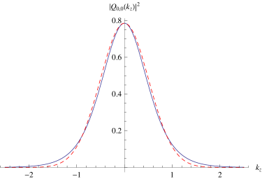
Figure 1: Geometric momentum distribution density for the ground state of ground rotational state $Y_{0,0}=1/(\sqrt{4\pi})$ (solid line), and the momentum distribution density for the ground state of one-dimensional simple harmonic oscillator (dashed line). They are almost identical. In all figures, the dimensionless momentum $k_{z}\equiv p_{z}/\hbar$ is used.

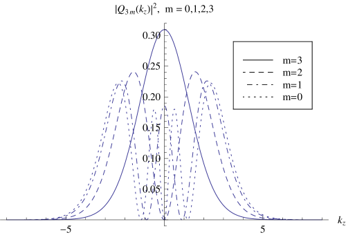
Figure 2: Geometric momentum distribution density for the rotational states $Y_{lm}(\theta,\varphi)$ with $l=1$ and $m=0,1,2,3$, they have number of nodes $3,2,1,0$ respectively. It is worthy of stressing that for a given set ($l,m$), i.e. each curve in this figure, behaves like a stationary harmonic oscillator state.

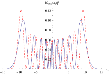
Figure 3: Geometric momentum distribution density for rotational state $Y_{10,0}(\theta,\varphi)$ (solid line), and the momentum distribution density for the $10$th excited state of one-dimensional simple harmonic oscillator (dashed line). Since both probabilities in a small interval $\Delta k_{z}$ are almost the same, they have the same classical limit: the simple harmonic oscillation.

The rotation of a homonuclear diatomic molecule around its center of mass, and the free rotation of spherical cage molecule $C_{60}$ or $Au_{32}$ gong  around its center, etc.rotator5 , can be well modelled by a spherical top. Here, there is a quantum uncertainty associated with degree of freedom $r$, but we can choose a confining potential $V(r)$ such that the uncertainty is minimum as $\Delta r\Delta p_{r}=\hbar/2$. Then it raises a crucial problem: if we can subtract this radial momentum contribution from the total one, whether our results $|Q_{lm}(p_{z})|^{2}$ can be experimentally testable. Fortunately, the answer is affirmative, as shown below.

Resuming $p_{i}$ without multiplying the radius $r$ as doing in (18)-(20), and $[{x}_{{i}}{,p}_{j}]=i\hbar(\delta_{ij}-x_{i}x_{j}/r^{2}{)}$ liu11-1 . The ground state $Y_{00}(\theta,\varphi)=1/\sqrt{4\pi}$ is the minimum uncertainty state for three pairs of ($x_{i},p_{i}$) and $\Delta x_{i}\Delta p_{i}=\hbar/3$. The state $Y_{00}(\theta,\varphi)$ bears neither energy nor angular momentum, and the presence of zero-point the momentum fluctuation $\Delta p_{i}=\hbar/(\sqrt{3}r)$ contradicts what classical mechanics would indicate. With preparing these molecules into ground state of rotation, the probability density of the geometric momentum distribution is given by $|Q_{0,0}(p_{z})|^{2}$ (44). With $r\approx 5.0$Å for $C_{60}$, $\Delta p_{i}\approx 0.07a.u.$($1a.u.=\hbar/a_{0}$, with $a_{0}$ denoting the Bohr radius) and $r\approx 1.0$Å for $H_{2}$, $\Delta p_{i}\approx 0.3a.u.$ that seems within the resolution power of a recently designed momentum spectrometer PSpectr1 ; PSpectr2 ; PSpectr3 . Moreover, if it is possible to prepare these molecules into any excited states, the momentum distributions $|Q_{lm}(p_{z})|^{2}$ given by Eq. (34) have even high resolutions.

V Conclusions and Discussions

How to understand quantum motions on a surface had been considered out of the problem. This might be due to the fact that in elementary particle physics and quantum gravity, physicists were acquainted with a fact that the outer space of the universe had little effect on the inner one japan1993 . Thus, consideration of the extrinsic curvature of two-dimensional surfaces was thought sheer nonsense, and the intrinsic property of the surfaces suffices in physics, which does not depend on whether they are embedded into the three-dimensional Euclidean, even higher-dimensional, space or not japan1993 . However, recent experiments demonstrate that the energy spectrum on constrained motion on two-dimensional curved surface is significantly influenced by the geometric potential depending on the extrinsic curvature 2010-2 ; epl . We show that the geometric momentum is indispensable to the geometric potential, and even more fundamental.

For motions on two dimensional spherical surface $S^{2}$, there is a new dynamical symmetry obeying $SO(3,1)$ group whose six generators are the Cartesian components of the geometric momentum $\mathbf{p}$ and the orbital angular momentum $\mathbf{L}$, where the dependence of the geometric momentum on extrinsic curvature, the mean curvature, reflects an embedding effect. From the commutation relations $[{L}_{{i}}{,p}_{i}]=0$, $(i=1,2,3)$, we have three complete sets of commuting observables, and they are equivalent with each other upon a rotation of coordinates. Thus a novel dynamical representation based on two observables, ($p_{z},L_{z}$) in the present paper, is successfully constructed, and any states on $S^{2}$ can go through a momentum analysis.

Because the free rotation is ubiquitous in microscopic domain, we propose to measure the momentum distribution of the state represented by spherical harmonics to probe the embedding effect, once preparing the some molecules into the state. This kind of experiments seems within reach of the present nanotechnological capabilities PSpectr1 ; PSpectr2 ; PSpectr3 ; rotator1 ; rotator2 ; rotator3 ; rotator4 .

References

• (1) P. A. M. Dirac, The Principles of Quantum Mechanics, 4th ed. (Oxford University Press, Oxford, 1967).
• (2) P. A. M. Dirac, Lectures on quantum mechanics (Yeshiva University, New York, 1964); Can. J. Math. 2, 129(1950).
• (3) H. Jensen and H. Koppe, Ann. Phys. 63, 586(1971).
• (4) R. C. T. da Costa, Phys. Rev. A 23, 1982(1981).
• (5) M. Ikegami and Y. Nagaoka, S. Takagi and T. Tanzawa, Prog. Theoret. Phys. 88, 229(1992).
• (6) H. Kleinert and S. V. Shabanov, Phys. Lett. A 232, 327(1997).
• (7) L. Kaplan, N. T. Maitra and E. J. Heller, Phys. Rev. A 56, 2592(1997).
• (8) J. R. Klauder, S. V. Shabanov, Nucl. Phys. B 511, 713(1998).
• (9) G. Ferrari and G. Cuoghi, Phys. Rev. Lett. 100, 230403 (2008).
• (10) B. Jensen and R. Dandoloff, Phys. Rev. A 80, 052109 (2009).
• (11) C. Ortix and J. van den Brink, Phys. Rev. B 81, 165419 (2010); Phys. Rev. B 83, 113406 (2011).
• (12) Q. H. Liu, L. H. Tang, D. M. Xun, Phys. Rev. A 84, 042101(2011).
• (13) M. V. Entin and L. I. Magarill, Phys. Rev. B 64, 085330(2001). It is worthy of mentioning that one may wonder whether the momentum in the spin-orbit coupling electrons on a curved surface might be with the geometric momentum. It is not the case exactly. A proper treatment needs to start from the spin-orbit coupling term $\hbar/(4m^{2})\mathbf{S}\cdot(\nabla V\times\mathbf{P})$ in three-dimensional flat space then confining it on the curved surface, where $V$ is the crystal potential, $\mathbf{P}$ the electron momentum and $\mathbf{S}$ the spin operator, and the relation between the resultant expression and the geometric momentum is explored in depth.
• (14) A.V. Chaplik and L. I. Magarill, Phys. Rev. Lett. 96, 126402 (2006).
• (15) M. P. López-Sancho and M. C. Muñoz, Phys. Rev. B 83, 075406 (2011).
• (16) Erhu Zhang, Shengli Zhang, and Qi Wang, Phys. Rev. B 75, 085308(2007).
• (17) A. Szameit, et. al, Phys. Rev. Lett. 104, 150403(2010).
• (18) J. Onoe, T. Ito, H. Shima, H. Yoshioka and S. Kimura, Europhys. Lett. 98, 27001(2012).
• (19) Dirac’s theory for a systems with second class constraints is not compatible with the Schrödinger’s theory for the system. For instance, for quantum potential, Schrödinger’s theory gives an unique result $V_{g}=-\hbar^{2}/(2\mu)(M^{2}-K)$, whereas the Dirac’s theory gives $V_{g}=-\hbar^{2}/(2\mu)(\alpha M^{2}-\beta K)$  1992 with $\alpha$ and $\beta$ two real parameters provided that Dirac bracket $\{f{,g\}}_{D}$ between two variables $f$ and $g$ in the theory is taken as the restriction of the symplectic form to the constraint surface in phase space. This compatibility problem is discussed in Ref. 1992 . However, I put forward a conjecture liu11-1 that the arbitrariness with $\alpha$ and $\beta$ can be fixed as $\alpha=\beta=1$ once a correspondence of the equation of motion for the momentum $\left[p_{i},H\right]/(i\hbar)\rightleftarrows\{p_{i}{,H\}}_{D}$ is imposed as a fundamental relation in the canonical quantization procedure.
• (20) E. W Weisstein, ”Intrinsic Curvature.” From MathWorld–A Wolfram Web Resource. http://mathworld.wolfram.com/IntrinsicCurvature.html
• (21) The terminology geometric potential was firstly introduced in A. V. Chaplik and R. H. Blick, New J. Phys. 6, 33(2004), and the embedding potential was used in japan1993 , the curvature potential in M. Encinosa and L. Mott, Phys. Rev. A 68, 014102 (2003), the quantum potential in P. Maraner, Ann. Phys. 246, 325 (1996) the effective geometry-induced quantum potential in V. Atanasov, R. Dandoloff, A. Saxena, Phys. Rev. B 79, 033404(2009), and the curvature-induced effective potential in H. Shima, H. Yoshioka, and J. Onoe, Phys. Rev. B 79, 201401(R) (2009), etc. I think that geometric potential and embedding potential are two appropriate names.
• (22) Q. H. Liu, C. L. Tong and M. M. Lai, J. Phys. A: Math. and Theor. 40, 4161(2007).
• (23) C. E. Weatherburn, Differential Geometry of Three Dimensions, Vol. 1. (Cambridge University Press, 1930).
• (24) S. Matsutani, J. Phys. A: Math. Gen. 26, 5133(1993).
• (25) M. Vos, I. McCarthy, Am. J. Phys. 65, 544(1997), M. Vos, Aust. J. Phys. 51, 609(1998).
• (26) E. Weigold, I. McCarthy, Electron Momentum Spectroscopy (Kluwer Academic/Plenum, New York, 1999).
• (27) Q. H. Liu, and T. G., Liu, Int. J. Theor. Phys. 42, 2877(2003).
• (28) X. M. Zhu, M. Xu, and Q. H. Liu, Int. J. Geom. Meth. Mod. Phys. 3, 411(2010).
• (29) D. M. Xun, and Q. H. Liu, Int. J. Geom. Meth. Mod. Phys. 10, 1220031(2013).
• (30) For motions on a spherical surface, the initial constraint equation can be either $x^{2}+$ $y^{2}+z^{2}=r^{2}$ or $x\dot{x}+$ $y\dot{y}+z\dot{z}=0$ where $\dot{x}_{i}\equiv dx_{i}/dt$. The Dirac’s theory for constrained systems can also give the geometric momentum. The calculations are available in references: T. Homma, T. Inamoto, T. Miyazaki, Phys. Rev. D 42, 2049(1990), and T. Matsunaga, T. Miyazaki, M. Nojiri, C. Ohzeki and M. Yamanobe, Nuovo Cimento B, 113, 975(1998). Unfortunately, in all these treatments, there are infinitely many sets of generalized momentum, each of them corresponds to a set of the local coordinates parameterizing the curved two-dimensional surface, including the geometric momentum. In order to single out the geometric momentum, a correspondence of the equation of motion for the momentum set $\left[p_{i},H\right]/(i\hbar)\rightleftarrows\{p_{i}{,H\}}_{D}$ must be imposed, as proposed and discussed in Ref. liu11-1 .
• (31) H. R. Sun, D. M. Xun, L. H. Tang, and Q. H. Liu, Commun. Theor. Phys. 58, 31(2012).
• (32) J. J. Sakurai, Modern Quantum Mechanics, Revised Edition (Addison-Wesley, New York. 2005).
• (33) J. P. Dahl and M. Springborg, J. Chem. Phys. 88, 4535 (1988).
• (34) M. Ji, X. Gu, X. Li, X. G. Gong, J. Li, and L. S. Wang, Angew. Chem. Int. Ed. 44, 7119-7123(2005).
• (35) B. Coutant, and P. Brechignac, J. Chem. Phys. 91, 1978-1986(1989).
• (36) M. Vos, S. A. Canney, I. E. McCarthy, S. Utteridge, M. T. Michalewicz, and E. Weigold, Phys. Rev. B 56, 1309-1315(1997).
• (37) X. G. Ren, C. G. Ning, J. K. Deng, S. F. Zhang, G. L. Su, B. Li, and X. J. Chen, Chinese Phys. Lett. 22, 1382(2005).
• (38) M. Kjellberg, O. Johansson, F. Jonsson, A.V. Bulgakov, C. Bordas, E. E. B. Campbell, K. Hansen, Phys. Rev. A 81, 023202(2010).
• (39) B. C. Stipe, M. A. Rezaei and W. Ho, Science 279, 1907(1998).
• (40) J. Neumann, K. E. Gottschalk, and R. D. Astumian, ACS Nano. 6, 5242-8(2012).
• (41) N. Néel, L. Limot, J. Kröger, and R. Berndt, Phys. Rev. B. 77, 125431(2008).
• (42) J. Michl, and E. C. Sykes, ACS Nano. 3, 1042(2009).