SOME ASPECTS OF OPTICAL SPATIAL SOLITONS IN PHOTOREFRACTIVE CRYSTALS

Abstract

We have reviewed recent developments of some aspects of optical spatial solitons in photorefractive media. Underlying principles governing the dynamics of photorefractive nonlinearity have been discussed using band transport model. Nonlinear dynamical equations for propagating solitons have been derived considering single as well as two-photon photorefractive processes. Fundamental properties of three types of solitons, particularly, screening, photovoltaic and screening photovoltaic solitons have been considered. For each type of solitons, three different configurations i.e., bright, dark and gray varieties have been considered. Mechanisms of formation of these solitons due to single as well as two-photon photorefractive processes have been considered and their self bending discussed. Vector solitons, particularly, incoherently coupled solitons due to single photon and two-photon photorefractive phenomena have been highlighted. Existence of some missing solitons have been also pointed out.

1 Introduction

The advent of nonlinear optics has paved the way to a number of fundamental discoveries. Exotic one, among many of these, is the discovery of optical solitons  [1, 2, 3, 4, 5, 6, 7, 8, 9, 10, 11, 12, 13, 14, 15, 16]. These are optical pulses or beams which are able to propagate without broadening and distortion. Optical solitons are envelope solitons, and the term soliton was first coined by Zabusky and Kruskal in 1965 to reflect the particle like nature of these waves that remain intact even after mutual collision  [4]. Optical solitons are extensively studied topic not solely due to their mathematical and physical elegance but as well as due to the possibility of real life applications. They have been contemplated as the building blocks of soliton based optical communication systems, signal processing, all optical switching, all optical devices etc.

In optics, three different types of solitons are known till date, these are, temporal  [2, 3], spatial [5, 6] and spatio-temporal solitons [7, 8]. Temporal solitons are short optical pulses which maintain their temporal shape while propagating over long distance. The way a temporal optical soliton is established is that a nonlinear pulse sets out in dispersive medium and develops a chirp. Then the dispersion produces a chirp of opposite sign. A temporal soliton pulse results due to the balancing of these opposite chirps across the width of the pulse, which arise from the material dispersion and nonlinearity.These opposite chirps balance each other when dispersion is completely canceled by the nonlinearity of the medium. Temporal solitons are routinely generated in optical fibers [2] and they are backbone of soliton based optical communication systems, soliton lasers etc. In contrast, optical spatial solitons are beams of electromagnetic energy that rely upon balancing diffraction and nonlinearity to retain their shape. While propagating in the nonlinear medium, the optical beam modifies the refractive index of the medium in such a way that the spreading due to diffraction is eliminated. Thus, optical beam induces a nonlinear waveguide and at the same time guided in the waveguide it has induced. This means soliton is a guided mode of the nonlinear waveguide induced by it.

Though temporal solitons can be easily generated in optical fibers, generation of spatial optical solitons is a much more difficult task. For example, in silica glass, the nonlinearity is proportional to light intensity and the value of the proportionality constant $n_{2}$ is of the order of $10^{-16}cm^{2}/W$ only. Therefore, in order to compensate for the beam spreading due to diffraction, which is a large effect, required optical nonlinearity is very large, and, consequently optical power density is also large [8]. Another impediment in detecting spatial solitons, in bulk Kerr nonlinear media, is the catastrophic collapse of the optical beam, which is inevitable with Kerr nonlinearity. Discovery of non Kerr nonlinearities, whose mechanism is different from Kerr nonlinearity, has lead to the revelation of stable three dimensional soliton formations without catastrophic collapse. These nonlinearities are photorefractive nonlinearity [10, 18], quadratic nonlinearity [19, 20, 21, 22] and resonant electronic nonlinearity in atoms or molecules [23, 24, 25, 26, 27]. With the identification of photorefractive nonlinearity, which possesses strong nonlinear optical response, it is possible to create optical solitons at very low light intensity. Spatial photorefractive optical solitons possess some unique properties which make them attractive in several applications, such as, all optical switching and routing, interconnects, parallel computing, optical storage etc [15, 16, 28, 35]. They are also promising for experimental verification of theoretical models, since, they can be created at very low power. In the present article, we confine our discussion on the properties of photorefractive spatial solitons.

2 Photorefractive Effect

The photorefractive(PR) effect is the change in refractive index of certain electro-optic materials owing to optically induced redistribution of charge carriers. Light induced refractive index change occurs owing to the creation of space charge field, which is formed due to nonuniform light intensity. Originally the photorefractive effect was considered to be undesirable, since this leads to scattering and distortion of collimated optical beams [36]. Soon it was realized that these materials have potential applications in holography [33], optical phase conjugation [32], optical signal processing and optical storage [34, 35]. Photorefractive materials are classified in three different categories. Most commonly used photorefractive materials are inorganics, such as, $LiNbO_{3}$, $BaTiO_{3}$, $Sr_{x}Br_{1-x}Nb_{2}O_{6}$, $KNbO_{3}$, $Bi_{12}SiO_{20}$, $Bi_{12}TiO_{20}(BTO)$ etc. Semiconductors have large carrier mobility that produces fast dielectric response time, which is important for fast image processing. Therefore, photorefractive semiconductors, such as, GaAs, InP, CdTe etc., complement the photorefractive ferroelectrics with the potential of fast holographic processing of optical information. Polymers also show strong photorefractive effect [37, 38, 39, 40]. They are easy to produce and PR effect in polymers appear only if a high voltage is applied. Strong photorefractive pattern can be erased easily in polymers by decreasing the applied voltage. Polymers show good temperature stability, and for a given applied voltage, they usually show stronger refractive index change in comparison to inorganic crystals with equal doping densities.

3 Origin of Photorefractive Nonlinearity

In a photorefractive material, the spatial distribution of intensity of the optical field gives rise to an inhomogeneous excitation of charge carriers. These charge carriers migrate due to drift and or diffusion and produce a space charge field, whose associated electric field modifies the refractive index of the crystal via Pockel’s effect [32, 34, 35]. For a noncentrosymmetric photorefractive crystal, the refractive index change due to the linear electro-optic effect is given by [32, 34]

$$\Delta n=-\frac{1}{2}n^{3}r_{eff}E_{sc},$$ (1)

where $n$ is the average refractive index, $r_{eff}$ is the effective linear electro-optic coefficient which depends on the orientation of the crystal and polarization of light, and $E_{sc}$ is the space charge field. A unique feature of photorefractive materials is their ability to exhibit both self focusing and defocusing nonlinearity in the same crystal. This is achieved by changing the polarity of the biased field, which in turn changes the polarity of the space charge field $E_{sc}$. Hence, the same crystal can be used to generate either bright ( require self focusing nonlinearity) or dark and gray solitons ( require defocusing nonlinearity). Photorefractive nonlinearity is also wavelength sensitive, thus, it is possible to generate solitons at one wavelength and then use the soliton supported channel to guide another beam at different wavelength.

4 Band Transport Model

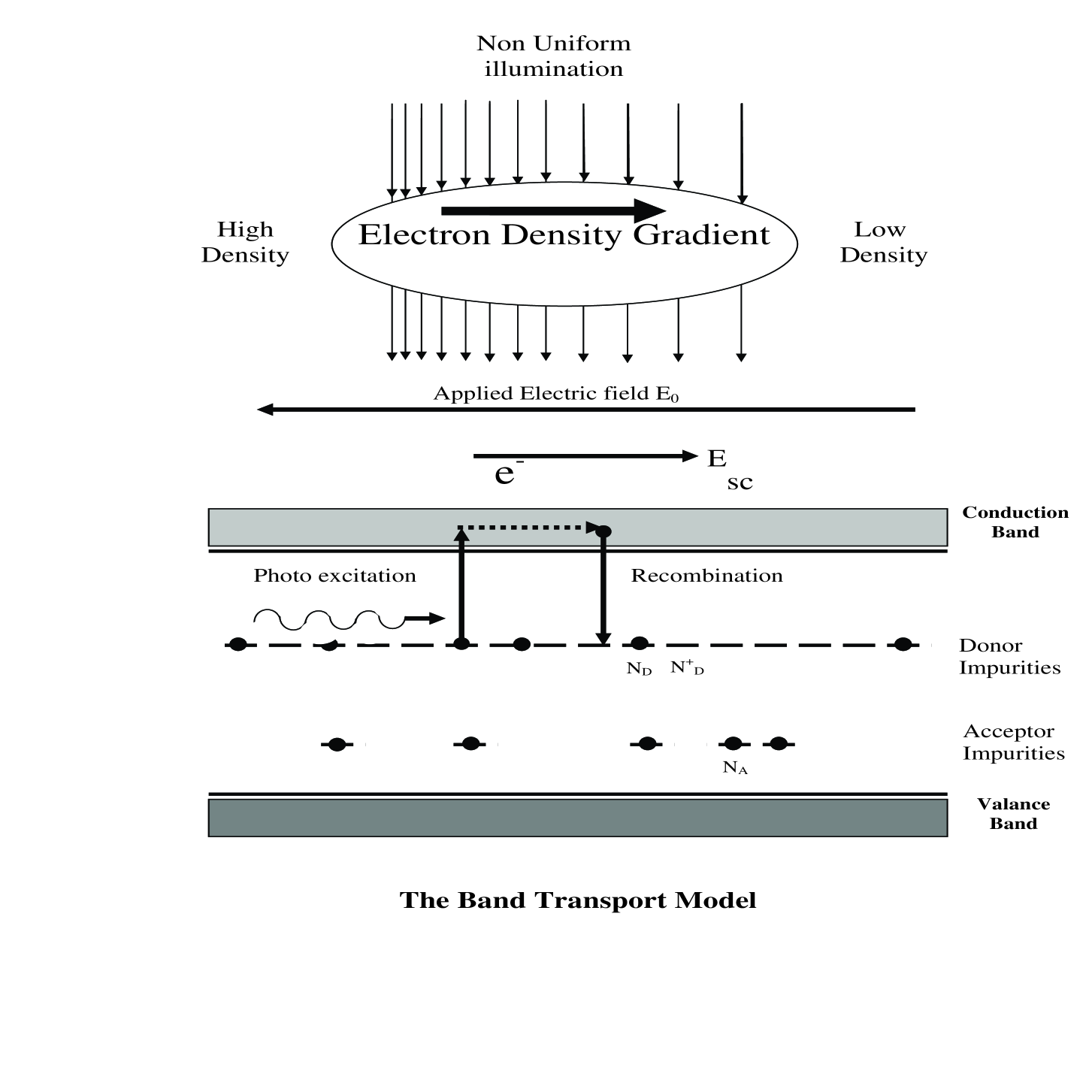
Figure 1: Band transport model

The most widely accepted theoretical formulation of photorefractive phenomenon is described by Kukhtarev-Vinetskii band transport model [41]. A schematic diagram of this model is shown in figure (1), where a PR crystal is being illuminated by an optical beam with nonuniform intensity.

Insert Figure (1) here

The photorefractive medium, at the ground level, has completely full valance band and an empty conduction band. The material has both donor and acceptor centers, uniformly distributed, whose energy states lies somewhere in the middle of the band gap. The acceptor electron states are at much lower energy in comparison to that of the donor electron states. The presence of a nonuniform light beam excites unionized donor impurities, creates charge carriers which move to the conduction band where they are free to move to diffuse or to drift under the combined influence of self generated and external electric field and are finally trapped by the acceptors. During this process, some of the electrons are captured by ionized donors and thus are neutralized. In the steady state, the process leads to the charge separation, which tends to be positive in the illuminated region and vanish in the dark region.

We assume that the donor impurity density is $N_{D}$ and acceptor impurity density $N_{A}$. If the ionized donor density is $N_{D}^{+}$, then the rate of electron generation due to light and thermal processess is $(s_{i}I+\beta_{T})(N_{D}-N_{D}^{+}),$ where $s_{i}$ is the cross section of photoexcitation, $I$ is the intensity of light which is written in terms of Poynting flux $I=\frac{n}{2\eta_{0}}|\Phi|^{2}$ , $\Phi$ is the electric field of light, $\epsilon_{0}$ is the free space permittivity, and $\beta_{T}$ is the rate of thermal generation. If $N$ is the electron density and $\gamma_{R}$ the electron trap recombination coefficient, then, the rate of recombination of ionized donars with free electrons is $\gamma_{R}NN_{D}^{+}$. Thus, the rate equation describing the donar ionization is given by

$$\frac{\partial N_{D}^{+}}{\partial t}=(s_{i}I+\beta_{T})(N_{D}-N_{D}^{+})-\gamma_{R}NN_{D}^{+}.$$ (2)

The electron concentration is affected by recombination with ionized donors and due to migration of electrons, resulting in an electron current with current density $J$, hence, electron continuity equation turns out to be

$$\frac{\partial N}{\partial t}-\frac{\partial N_{D}^{+}}{\partial t}=\frac{1}{e}\overrightarrow{\nabla}.\overrightarrow{J},$$ (3)

and

$$\overrightarrow{J}=eN\mu\overrightarrow{E}+k_{B}T\mu\overrightarrow{\nabla}N+k_{p}s_{i}\left(N_{D}-N_{D}^{+}\right)I\vec{c},$$ (4)

where the current density $\overrightarrow{J}$ is the sum of the contributions from the drift, diffusion and photovoltaic effect; $e$ is the electronic charge, $\mu$ is the electron mobility, $k_{B}$ is the Boltzmann constant, $T$ is electron temperature, $k_{p}$ is the photovoltaic constant and $\vec{c}$ is the unit vector in the direction of c-axis of the PR crystal. $E$ is the total electric field including the one externally applied and that associated with the generated space charge. The redistribution of electrical charges and the creation of space charge field obey the Poisson’s equation, therefore,

$$\overrightarrow{\nabla}\cdot\epsilon\overrightarrow{E}=\rho,$$ (5)

and the charge density $\rho$ is given by

$$\rho\left(\overrightarrow{r}\right)=e\left(N_{D}^{+}-N_{A}-N\right).$$ (6)

Equations (2) -(6) can be solved to find out the space charge field $E_{sc}$ and subsequently the optical nonlinearity in the photorefractive media.

5 Space Charge Field

To estimate the nonlinear index change in photorefractive media due to the presence of nonuniform optical field, we need to calculate the screening electric field $E_{sc}$. The response of a photorefractive material to the applied optical field is anisotropic and it is nonlocal function of light intensity. Anisotropy does not allow radially symmetric photorefractive solitons [42, 43]. To formulate a simple problem, and since, most of the experimental investigations on photorefractive solitons are one dimensional waves, it is appropriate to find material response in one dimension ( say x only). Steady state photorefractive solitons may be obtained under homogeneous background illumination, which enhances dark conductivity of the crystal. In the steady state, induced space charge field $E_{sc}$ can be obtained from the set of rate, continuity, current equations and Gauss law. In the steady state, and in one dimension, these equations reduce to [44, 45, 46]:

$$s_{i}(I+I_{d})(N_{D}-N_{D}^{+})-\gamma_{R}NN_{D}^{+}=0,$$ (7)

$$\frac{\partial E_{sc}}{\partial x}=\frac{e}{\epsilon_{0}\epsilon_{r}}(N_{D}^{+}-N_{A}-N),$$ (8)

$$J=eN\mu E_{sc}+k_{B}T\mu\frac{\partial N}{\partial x}+k_{p}s_{i}\left(N_{D}-N_{D}^{+}\right)I,$$ (9)

$$\frac{\partial J}{\partial x}=0,$$ (10)

where $\epsilon_{r}$ is the relative static permittivity; $I_{d}(=\frac{\beta_{T}}{s_{i}})$ is the so called dark irradiance that phenomenologically accounts for the rate of thermally generated electrons. This is also the homogeneous intensity that controls the conductivity of the crystal. In most cases, the optical intensity $I$ is such that for electron dominated photo-refraction, $N\ll N_{D}$, $N\ll N_{A}$ and $N_{A}\ll N_{D}^{+}$. Under this usually valid situation, the space charge field $E_{sc}$ is related to the optical intensity $I$ through

$$E_{sc}=E_{0}\frac{I_{\infty}+I_{D}}{I+I_{D}}+E_{p}\frac{I_{\infty}-I}{I+I_{D}}-\frac{k_{B}T}{e}\frac{1}{I+I_{D}}\frac{\partial I}{\partial x},$$ (11)

where $E_{o}$ is the external bias field to the photorefractive crystal, $E_{p}=\frac{k_{p}\gamma_{R}N_{A}}{e\mu}$ is the photovoltaic field. In addition, we have assumed that the power density of the optical field attains asymptotically a constant value at $x\rightarrow\pm\infty$ i.e., $I(x\rightarrow\pm\infty,z)=I_{\infty}$. Moreover, in the region of constant illumination, equations(7)-(10) require that the space charge field $E_{sc}$ is independent of $x$ i.e., $E_{sc}(x\rightarrow\pm\infty,z)=E_{o}$.

6 Photorefractive Nonlinearity

The space charge induced change $\triangle n$ in the refractive index $n$ is obtained as

$$|\triangle n|=\frac{1}{2}n^{3}r_{eff}\left[E_{0}\frac{I_{\infty}+I_{D}}{I+I_{D}}+E_{p}\frac{I_{\infty}-I}{I+I_{D}}-\frac{k_{B}T}{e}\frac{1}{I+I_{D}}\frac{\partial I}{\partial x}\right].$$ (12)

It is evident from above expression that the change in refractive index is intensity dependent, i.e., under the action of nonuniform illumination the photorefractive crystal has become an optical nonlinear medium. The first term in the above equation is generally known as the screening term. In nonphotovoltaic photorefractive material, this is the main term which is responsible for soliton formation. The space charge redistribution in a photorefractive crystal is caused mainly by the drift of photoexcited charges under a biasing electric field. This mechanism leads directly to a local change of refractive index and is responsible for self-focusing of optical beams. The second term is due to photovoltaic effect, which leads to the formation of photovoltaic solitons. First two terms do not involve spatial integration, therefore, they are local nonlinear terms. Functional form of both terms are different from Kerr nonlinearity. These terms are similar to that of saturable nonlinearity and explain why the collapse phenomenon is not observable in photorefractive materials. Besides drift mechanism, transport of charge carriers occurs also due to diffusion process. This process results in the nonlocal contribution to the refractive index change. The last term is due to diffusion. The strength of the diffusion effect is determined by the width of the soliton forming optical beam. In case of strong bias field and relatively wide beams, the diffusion term is often neglected. However, its contribution can become significant for very narrow spatial solitons or optical beams. When diffusion is significant, it is responsible for deflection of photorefractive solitons [44, 45, 46].

7 Classification of Photorefractive Solitons

7.1 Solitons Due to Single Photon Photorefractive Phenomenon

Till date, three different types of steady state spatial solitons have been predicted in photorefractive media, which owe their existence due to single photon photorefractive phenomenon. Photorefractive screening solitons were identified first. In the steady state, both bright and dark screening solitons (SS) are possible when an external bias voltage is appropriately applied to a non-photovoltaic photorefractive crystal [47, 48, 49, 50, 51, 52, 53, 54, 55, 56]. Intuitively, the formation of bright screening photorefractive solitons can be understood as follows. When a narrow optical beam propagates through a biased photorefractive crystal, as a result of illumination, conductivity in the illuminated region increases and the resistivity decreases. Since the resistivity is not uniform across the crystal, the voltage drops primarily across the non illuminated region and voltage drop is minimum in the high intensity region. This leads to the formation of large space charge field in the dark region and much lower field in the illuminated region. The applied field is thus partially screened by the space charges induced by the soliton forming optical beam. The refractive index changes which is proportional to this space charge field. The balance of self diffraction of the optical beam by the focusing effect of the space charge field induced nonlinearity leads to the formation of spatial solitons. These screening solitons were first predicted by Segev et. al. [47], whereas, the experimental observation of bright SS were reported by M.Shih et. al. [48] and those of dark SS were reported by Z. Chen et. al. [49].

The second type PR soliton is the photovoltaic solitons  [57, 58, 59, 60, 61], the formation of which, however, requires an unbiased PR crystal that exhibits photovoltaic effect, i.e., generation of dc current in a medium illuminated by a light beam. The photovoltaic (PV) solitons owe their existence to bulk photovoltaic effect, which creates the space charge field, that, in turn modifies the refractive index and gives rise to spatial solitons. These solitons were first predicted by G. C. Valey et. al. [57] and observed experimentally in 1D by M.Taya et.al. [58] and in 2D by Z.Chen et. al. [59]. Two dimensional bright photovoltaic spatial solitons were also observed in a Cu:KNSBN crystal by She et. al. [62]. The observed spatial solitons were broader than those predicted by considering $E_{sc}$ due to signal beam alone. This was satisfactorily explained by an equivalent field induced by the background field.

The third type of photorefractive solitons arises when an electric field is applied to a photovoltaic photorefractive crystal [31, 60, 61, 63, 64]. These solitons, owe their existence to both photovoltaic effect and spatially nonuniform screening of the applied field, and, are also known as screening photovoltaic (SP) solitons. It has been verified that, if the bias field is much stronger than the photovoltaic field, then, the screening photovoltaic solitons are just like screening solitons. On the other hand, if the applied field is absent, then SP solitons degenerate into photovoltaic solitons in the closed circuit condition. The first observation of bright photovoltaic screening solitons in $LiNbO_{3}$ was reported by E. Fazio et. al. [31].

7.2 Nonlinear Equation for Solitons

In order to develop a semi analytical theory, one dimensional reduction is introduced in the subsequent discussion. The optical beam is such that no y dynamics is involved and it is permitted to diffract only along $x$ direction. Electric field $\overrightarrow{E}$ of the optical wave and the bias field $E_{0}$ are directed along the $x$ axis which is also the direction of the crystalline c-axis. Under this special arrangement, the perturbed extraordinary refractive index $\hat{n}_{e}$ is given by [45, 46, 60]

$$({\hat{n}_{e})^{2}}=n_{e}^{2}-n_{e}^{4}r_{eff}E_{sc},$$ (13)

where $n_{e}$is the unperturbed extraordinary index of refraction. This arrangement allows us to describe the optical beam propagation using Helmholtz’s equation for the electric field $\overrightarrow{E}$, which is as follows:

$$\nabla^{2}\overrightarrow{E}+(k_{0}\hat{n}_{e})^{2}\overrightarrow{E}=0,$$ (14)

where $k_{0}=\frac{2\pi}{\lambda_{0}}$ and $\lambda_{0}$ is the free space wavelength of the optical field. Moreover, if we assume $\overrightarrow{E}=\overrightarrow{x}\Phi(x,z)exp[i(kz-\omega t)],$ where $k=k_{0}n_{e}$ and employ slowly varying envelope approximation for the amplitude $\Phi$, then, the Helmholtz’s equation can be reduced to the following parabolic equation:

$$i\frac{\partial\Phi}{\partial z}+\frac{1}{2k}\frac{\partial^{2}\Phi}{\partial x^{2}}-\frac{1}{2}k_{0}n_{e}^{3}r_{eff}E_{sc}\Phi=0.$$ (15)

The space charge field that has been evaluated earlier in section(5) can be employed in the above equation to obtain following nonlinear Schrödinger equation:

$$i\frac{\partial A}{\partial\xi}+\frac{1}{2}\frac{\partial^{2}A}{\partial s^{2}}-\beta(1+\rho)\frac{A}{1+|A|^{2}}-\alpha\frac{(\rho-|A|^{2})A}{1+|A|^{2}}+\delta\frac{A}{1+|A|^{2}}\frac{\partial|A|^{2}}{\partial s}=0,$$ (16)

where $\xi=\frac{z}{k_{0}n_{e}x_{0}^{2}}$, $s=\frac{x}{x_{0}}$, $\rho=\frac{I_{\infty}}{I_{d}}$, $\beta=(k_{0}x_{0})^{2}(n_{e}^{4}r_{eff}/2)E_{0}$, $\alpha=(k_{0}x_{0})^{2}(n_{e}^{4}r_{eff}/2)E_{p}$, $A=\sqrt{\frac{n_{e}}{2\eta_{0}I_{d}}}\Phi$ and $\delta=(k_{0}^{2}x_{0}r_{eff}n_{e}^{4}k_{B}T)/(2e)$. Equation (16) gives rise to varieties of solitons depending on specific experimental situations. Important parameters which classify these solitons and govern their dynamics are $\alpha$ and $\beta$. The parameter $\delta$, which is associated with the diffusion term, is not directly responsible for soliton formation. The diffusion processes is primarily responsible for bending of trajectories of propagating solitons, hence, large value of $\delta$ influences the trajectory of bending. The dimensionless parameter $\beta$ can be positive or negative depending on the sign of $E_{0}$ i.e., the polarity of external applied field. In non-photovoltaic photorefractive media $\alpha=0$, therefore, if we neglect the diffusion term, which is small indeed, and introduce only first order correction, then $\beta$ is the parameter which governs the soliton formation. The relevant dynamical equation in non-photovoltaic photorefractive media turns out to be

$$i\frac{\partial A}{\partial\xi}+\frac{1}{2}\frac{\partial^{2}A}{\partial s^{2}}-\beta(1+\rho)\frac{A}{1+|A|^{2}}=0.$$ (17)

This is the modified nonlinear Schrödinger equation(MNLSE) with saturable nonlinearity which is not integrable. The term $1/(1+|A|^{2})$ represents local saturable nonlinear change of refractive index of the crystal induced by the optical beam. The saturating nature of the nonlinearity will be more clearly evident if we make the transformation $A=u\ exp[-i\beta(1+\rho)\xi]$, in which case above equation reduces to

$$i\frac{\partial u}{\partial\xi}+\frac{1}{2}\frac{\partial^{2}u}{\partial s^{2}}+\beta(1+\rho)\frac{|u|^{2}}{1+|u|^{2}}u=0.$$ (18)

It will be shown subsequently that a positive $\beta$ is essential for creation of bright spatial solitons, whereas, a negative $\beta$ leads to the formation of dark or gray solitons. Thus, by changing the polarity of the external applied field, it is possible to create bright as well as dark solitons in the same photorefractive media. Equation(17) has been extensively investigated for bright, dark as well as gray solitons [46, 60, 61]. In the next section, we consider bright screening spatial solitons using a method outlined by Christodoulides and Carvalho [46] and subsequently employed in a large number of investigations [108, 109, 110, 111, 137, 145, 146].

7.3 Bright Screening Spatial Solitons

We fist consider bright screening solitons for which the soliton forming beam should vanish at infinity $(s\rightarrow\pm\infty)$, and thus, $I_{\infty}=\rho=0$. Therefore, bright type solitary waves should satisfy

$$i\frac{\partial A}{\partial\xi}+\frac{1}{2}\frac{\partial^{2}A}{\partial s^{2}}-\beta\frac{A}{1+|A|^{2}}=0.$$ (19)

We can obtain stationary bright solitary wave solutions by expressing the beam envelope as $A(s,\xi)=p^{\frac{1}{2}}y(s)\exp(i\nu\xi)$, where $\nu$ is the nonlinear shift in propagation constant and y(s) is a normalized real function which is bounded as, $0\leq y(s)\leq 1.$ The quantity p represents the ratio of the peak intensity $(I_{max})$ to the dark irradiance $I_{d}$, where $I_{max}=I(s=0)$. Furthermore, for bright solitons, we require $y(0)=1$, $\dot{y}(0)=0$ and $y(s\rightarrow{\pm\infty})=0$ . Substitution of the ansatz for $A(s,\xi)$ into equation(19) yields

$$\frac{d^{2}y}{ds^{2}}-2\nu y-2\beta\frac{y}{1+py^{2}}=0.$$ (20)

Integration of above equation once and use of boundary condition yields

$$\nu=-(\beta/p)\ln(1+p),$$ (21)

and

$$\left(\frac{dy}{ds}\right)^{2}=(2\beta/p)[\ln(1+py^{2})-y^{2}\ln(1+p)].$$ (22)

By virtue of integration of above equation, we immediately obtain

$$s=\pm\frac{1}{(2\beta)^{1/2}}\int_{y}^{1}\frac{p^{1/2}}{[\ln(1+p\widehat{y}^{2})-\widehat{y}^{2}\ln(1+p)]^{1/2}}d\widehat{y}.$$ (23)

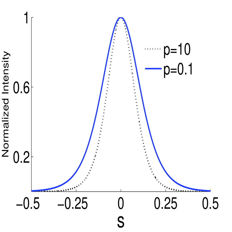
Figure 2: Normalized intensity profile of bright spatial solitons for $\beta=43,x_{0}=20\mu m;p=0.1$ and $10$.

The nature of above integrand is such that it does not provide any closed form solution. Nevertheless, the normalized bright profile $y(s)$ can be easily obtained by the use of simple numerical procedure. It can be easily shown that the quantity in the square bracket in equation(23) is always positive for all values of $y^{2}$ between $0\leq y(s)\leq 1$. Therefore, the bright screening photorefractive solitons can exist in a medium only when $\beta>0$ i.e., $E_{0}$ is positive. For a given value of $\beta$, the functional form of $y$ can be obtained for different p which determines soliton profile. For a given physical system, the spatial beam width of these solitons depends on two parameters $E_{0}$ and $p$. For illustration, we take SBN crystal with following parameters $n_{e}=2.35$, $r_{33}=224\times 10^{-12}$ m/V. Operating wavelength $\lambda_{0}=0.5\mu m$, $x_{0}=20\mu m$ and $E_{0}=2\times 10^{5}$ V/m. With these parameters, value of $\beta\simeq 43$. Figure (2) depicts typical normalized intensity profiles of bright solitons.

Insert Figure (2) here

7.3.1 Bistable Screening Solitons

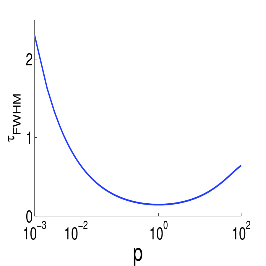
Figure 3: Variation of spatial width ($\tau_{FWHM}$) of solitons with power $p$. Figure shows existence of bistable solitons.

Equation(19) possesses several conserved quantities, one such quantity is $P=\int_{\infty}^{\infty}|A|^{2}ds$, which can be identified as the total power of the soliton forming optical beam. Numerically evaluated soliton profile $|A|^{2}=p|y(s)|^{2}$ can be employed to calculate $P$. Solitons obtained from equation(23) are stable since they obey Vakhitiov and Kolokolov [65] stability criteria i.e., $dP/d\nu>0$. These soliton profiles can be also employed to find out spatial width $\tau_{FWHM}$ ( full width at half maximum) of solitons. Figure (3) demonstrates the variation of spatial width $\tau_{FWHM}$ with $p$. This figure signifies the existence of two-state solitons, also known as bistable solitons, i.e., two solitons possessing same spatial width but different power. Similar bistable solitons were earlier predicted in doped fibers [66, 67]. However, these bistable solitons are different from those which were predicted by Kaplan and others [68], where two solitons with same power possessing two different nonlinear propagation constant.

Insert Figure (3) here

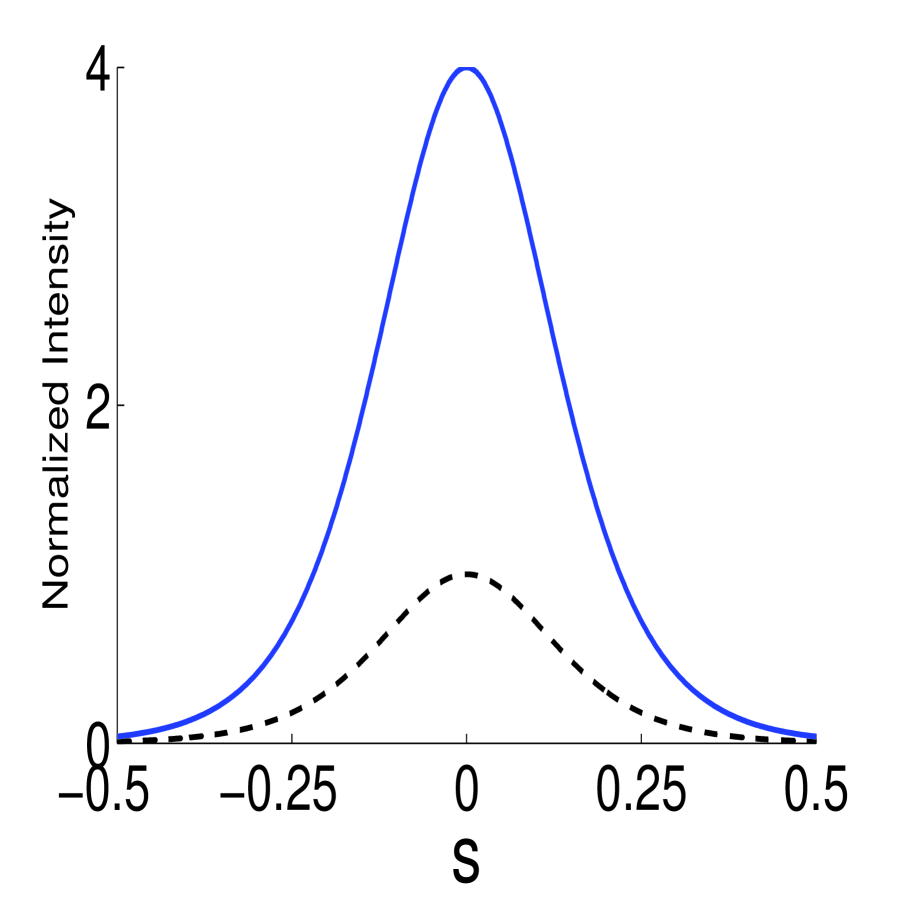
Figure 4: Normalized intensity profile of a pair of bistable solitons. Both solitons have same spatial width but they possess different peak power.

Another point worth mentioning is that, the $\tau_{FWHM}$ vs $p$ curve in figure(3) possesses local minimum, hence, it is evident that these solitons can exist only if their spatial width is above certain minimum value. This minimum value increases with the decrease in the value of $\beta$. For illustration, the shapes of a typical pair of bistable solitons with same $\tau_{FWHM}$ but different peak power have been depicted in figure(4). The dynamical behavior of these bistable solitons, while propagating, can be examined by full numerical simulation of equation(19), which confirms their stability.

Insert Figure (4) here

7.4 Dark Screening Solitons

Equation (17) also yields dark solitary wave solutions [46, 69], which exhibit anisotropic field profiles with respect to $s$. These solitons are embedded in a constant intensity background, therefore, $I_{\infty}$ is finite, hence, $\rho$ is also finite. To obtain stationary solutions, we assume $A(s,\xi)=\rho^{1/2}y(s)exp(i\nu\xi)$, where, like earlier case, $\nu$ is the nonlinear shift in propagation constant and $y(s)$ is a normalized real odd function of $s$. The profile $y(s)$ should satisfy following properties: $y(0)=0,y(s\rightarrow\pm\infty)=\pm 1,\frac{dy}{ds}=\frac{d^{2}y}{ds^{2}}=0$ as $s\rightarrow\pm\infty$. Substituting the form of A in equation(17) we obtain,

$$\frac{d^{2}y}{ds^{2}}-2\nu y-2\beta(1+\rho)\frac{y}{1+\rho y^{2}}=0.$$ (24)

Integrating above equation once and employing boundary condition, we get

$$\nu=-\beta.$$ (25)

Following similar procedure as employed earlier, we immediately obtain

$$s=\pm\frac{1}{(-2\beta)^{1/2}}\int_{y}^{0}\frac{d\widehat{y}}{[(\widehat{y}^{2}-1)-\frac{(1+\rho)}{\rho}\ln\frac{1+\rho\widehat{y}^{2}}{1+\rho}]^{1/2}}.$$ (26)

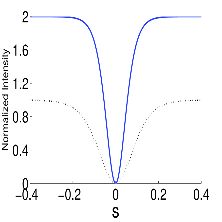
Figure 5: Normalised intensity profile of dark spatial solitons for $\beta=-43,x_{0}=20\mu m;\rho=1$ and $2$.

The quantity within the square bracket in equation(26) is always positive for all values of $y^{2}\leq 1$, thus $\beta$ i.e., $E_{0}$ must be negative so that r.h.s of equation(26) is not imaginary. An important point to note is that, for a particular type of photorefractive material, for example SBN, if positive polarity of $E_{0}$ is required for bright solitons, then one can observe dark solitons by changing polarity of $E_{0}$ . Spatial width of these solitons depends on only two variables $\beta$ and $\rho$ i.e., $E_{0}$ and $I_{\infty}$. It has been confirmed that, unlike their bright counterpart, dark screening photovoltaic solitons do not possess bistable property. For illustration, we take the same SBN crystal with other parameters unchanged, except in the present case $E_{0}=-2\times 10^{5}$ V/m. Therefore $\beta\approx-43$. Figure (5) depicts normalized intensity profiles of dark solitons which are numerically identified using equation(26).

Insert Figure (5) here

7.5 Gray Screening Solitons

Besides bright and dark solitons, equation (17) also admits another interesting class of solitary waves, which are known as gray solitons [46]. In this case too, wave power density attains a constant value at infinity i.e., $I_{\infty}$ is finite, and hence, $\rho$ is finite. To obtain stationary solutions, we assume

$$A(s,\xi)=\rho^{1/2}y(s)\exp[i(\nu\xi+\int^{s}\frac{Jd\widehat{s}}{y^{2}(\widehat{s})})],$$ (27)

where $\nu$ is again the nonlinear shift in propagation constant, $y(s)$ is a normalized real even function of $s$ and $J$ is a real constant to be determined. The normalized real function satisfies the boundary conditions $y^{2}(0)=m(0<m<1)$, i.e., the intensity is finite at the origin, $\dot{y(0)}=0$, $y(s\rightarrow\pm\infty)=1$ and all derivatives of $y(s)$ are zero at infinity. The parameter m describes grayness, i.e., the intensity $I(0)$ at the beam center is $I(0)=mI_{\infty}$. Substitution of the above ansatz for A in equation(17) yeilds

$$\frac{d^{2}y}{ds^{2}}-2\nu y-2\beta(1+\rho)\frac{y}{1+\rho y^{2}}-\frac{J^{2}}{y^{3}}=0.$$ (28)

Employing boundary conditions on y at infinity we obtain

$$J^{2}=-2(\nu+\beta).$$ (29)

Integrating equation(28) once and employing appropriate boundary condition, we immediately obtain

$$\nu=\frac{-\beta}{(m-1)^{2}}\left[\frac{m(1+\rho)}{\rho}\ln\left(\frac{1+\rho m}{1+\rho}\right)+1-m\right].$$ (30)

Finally

$$\left(\frac{dy}{ds}\right)^{2}=2\nu(y^{2}-1)+\frac{2\beta}{\rho}(1+\rho)\ln\left(\frac{1+\rho y^{2}}{1+\rho}\right)+2(\nu+\beta)\left(\frac{1-y^{2}}{y^{2}}\right).$$ (31)

The normalized amplitude $y(s)$ can be obtained by numerical integration of above equation. Note that dark solitons are a generalization of these gray solitons. Unlike bright or dark solitons, the phase of gray solitons is not constant across $s$, instead varies across $s$. Existence of these solitary waves are possible only when $\beta<1$ and $m<1$.

7.6 Self Deflection of Bright Screening Solitons

In the foregoing discussion we have neglected diffusion, however, the effect of diffusion cannot be neglected when solitons spatial width is comparable with the diffusion length. The diffusion process introduces asymmetric contribution in the refractive index change which causes solitons to deflect during propagation. Results of large number of investigations addressing the deflection of photorefractive spatial solitons in both non-centrosymmetric and centrosymmetric photorefractive crystals are now available [70, 71, 72, 73, 74, 75, 76, 77, 78, 79, 80, 81, 82]. Several authors have investigated self bending phenomenon using perturbative procedure [83, 84]. In this section, we employ a method of nonlinear optics [85, 86] which is different from perturbative approach. To begin with, we take finite $\delta$ and use the following equation to study the self bending of screening bright spatial solitons

$$i\frac{\partial A}{\partial\xi}+\frac{1}{2}\frac{\partial^{2}A}{\partial s^{2}}-\beta\frac{A}{(1+|A|^{2})}+\delta\frac{A}{(1+|A|^{2})}\frac{\partial(|A|^{2})}{\partial s}=0.$$ (32)

To obtain stationary solitary waves, we make use of the ansatz

$$A(s,\xi)=A_{0}(s,\xi)\exp[-i\Omega(s,\xi)],$$ (33)

in equation(32). A straightforward calculation yields following equations:

$$\frac{\partial A_{0}}{\partial\xi}-\frac{\partial A_{0}}{\partial s}\frac{\partial\Omega}{\partial s}-\frac{1}{2}A_{0}\frac{\partial^{2}\Omega}{\partial s^{2}}=0,$$ (34)

and

$$A_{0}\frac{\partial\Omega}{\partial\xi}+\frac{1}{2}\frac{\partial^{2}A_{0}}{\partial s^{2}}-\frac{1}{2}A_{0}\left(\frac{\partial\Omega}{\partial s}\right)^{2}-\beta\frac{A_{0}}{1+A_{0}^{2}}+\frac{\delta}{1+A_{0}^{2}}\frac{\partial(A_{0}^{2})}{\partial s}=0.$$ (35)

We look for a self-similar solution of (34) and (35) of the form

$$A_{0}=\frac{A_{00}}{\sqrt{f(\xi)}}exp\left[-\frac{({s-s_{0}(\xi)})^{2}}{2r_{0}^{2}f^{2}(\xi)}\right],$$ (36)

$$\Omega(s,\xi)=\frac{(s-s_{0}(\xi))^{2}}{2}\Lambda_{1}(\xi)+(s-s_{0}(\xi))\Lambda_{2}(\xi)+\Lambda_{3}(\xi),$$ (37)

$$\Lambda_{1}=-\frac{1}{f(\xi)}\frac{df}{d\xi},\ \ \ \ \ and\ \ \ \ \ \Lambda_{2}=-\frac{ds_{0}}{d\xi},$$ (38)

where, $r_{0}$ is a constant and $f(\xi)$ is a parameter which together with $r_{0}$ describe spatial width; in particular, $r_{0}f(\xi)$ is the spatial width of the soliton and $\Lambda_{3}$ is an arbitrary longitudinal phase function. $s_{0}(\xi)$ is the location of the center of the soliton. For a nondiverging/ nonconverging soliton, $f(\xi)=1$. Moreover, we assume that initially solitons are nondiverging i.e., $\frac{df(\xi)}{d\xi}=0$ at $\xi=0$. Substituting for $A_{0}$ and $\Omega$ in equation(35) and equating coefficients of $s$ and $s^{2}$ on both sides, we obtain

$$\frac{d^{2}f}{d\xi^{2}}=\frac{1}{r_{0}^{4}f^{3}}-\beta\frac{2A_{00}^{2}}{r_{0}^{2}f^{2}}\left(1+\frac{A_{00}^{2}}{f}\right)^{-2},$$ (39)

and

$$\frac{d^{2}s_{0}(\xi)}{d\xi^{2}}=-\delta\frac{2A_{00}^{2}}{r_{0}^{2}f^{3}}\left(1+\frac{A_{00}^{2}}{f}\right)^{-1}.$$ (40)

Equation(39) describes the dynamics of the width of soliton as it propagates in the medium, while equation(40) governs the dynamics of the centre of the soliton. In order to find out how a stationary soliton deviates from its initial propagation direction, we first solve equation(39) for stationary soliton states. From equation(39), condition for stationary soliton states can be obtained as

$$r_{0}=\left[\frac{(1+A_{00}^{2})^{2}}{2\beta A_{00}^{2}}\right]^{1/2}.$$ (41)

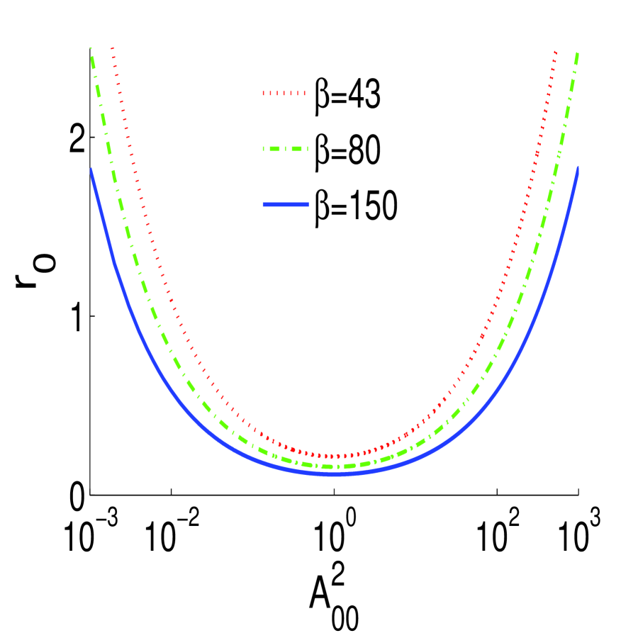
Figure 6: Existence curve of stationary solitons for different $\beta$.

Insert Figure (6) here

Figure (6) depicts variation of solitons spatial width with the normalized peak power $A_{00}^{2}$ . The curve in figure (6) is the existence curve of stationary solitons. Each point on this curve signifies the existence of a stationary soliton with a given spatial width and peak power. A stationary soliton of specific power and width as described by equation(41) deviates from its initial path which can be found out by integrating equation(40). The equation of trajectory of the center of soliton is

$$s_{0}(\xi)=-\frac{\Theta}{2}\xi^{2}+s_{00},$$ (42)

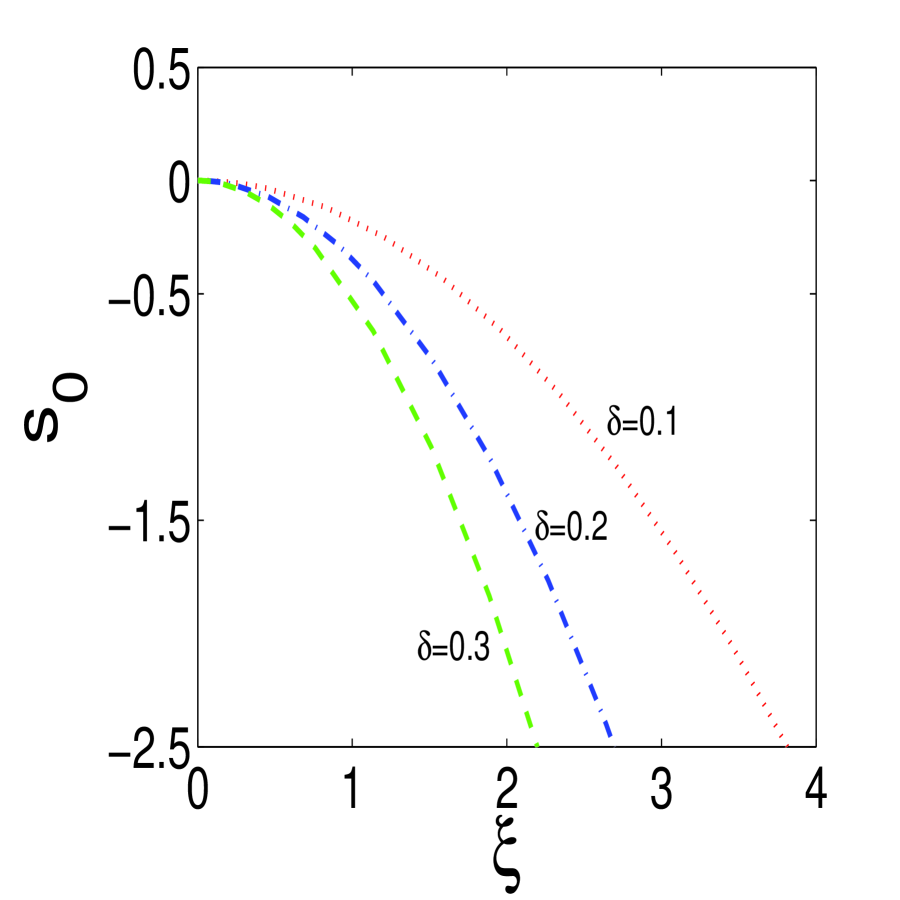
Figure 7: Spatial shift of soliton centre as it propagates through the photovoltaic crystal. $A_{00}=0.42$ and $r_{0}=0.298$.

where $\Theta=\delta\frac{2A_{00}^{2}}{r_{0}^{2}}(1+A_{00}^{2})$, $s_{00}=s_{0}(\xi=0)$, moreover $f=1$, since we are only interested in stationary solitons whose spatial shape remain invariant. Thus, the beam center follows a parabolic trajectory. The displacement of the soliton center with propagation distance has been depicted in figure (7). It is evident that the peak power of soliton influences lateral displacement of the soliton centre. The lateral displacement suffered by the spatial soliton is given by $\frac{\Theta}{2}\xi^{2}$. Equation(42) implies that the angular displacement of the soliton center shifts linearly with the propagation distance $\xi$. The more explicit expression of the angular displacement, i.e., the angle between the center of the soliton and the z axis can be easily obtained as $\Theta\xi$.

Insert Figure (7) here

7.7 Photovoltaic and Screening Photovoltaic Solitons

Steady state photovoltaic solitons can be created in a photovoltaic photorefractive crystal without a bias field. These photovoltaic solitons result from the photovoltaic effect [57, 58, 59, 60, 61] . Recently, it has been predicted theoretically that the screening-photovoltaic(SP) solitons are observable in the steady state when an external electric field is applied to a photovoltaic photorefractive crystal [31, 78]. These SP solitons result from both the photovoltaic effect and spatially nonuniform screening of the applied field.

If the bias field is much stronger in comparison to the photovoltaic field, then the SP solitons are just like the screening solitons. In absence of the applied field, the SP solitons degenerate into photovoltaic solitons in the close-circuit condition. In other words, a closed-circuit photovoltaic soliton or screening soliton is a special case of the SP soliton. Thus, in the subsequent analysis, we develop theory for SP solitons and obtain solutions of photovoltaic solitons as a special case. When the diffusion process is ignored, the dynamics of these steady-state screening PV solitons ( bright, dark and gray) can be examined [60, 78, 88] using the following equation

$$i\frac{\partial A}{\partial\xi}+\frac{1}{2}\frac{\partial^{2}A}{\partial s^{2}}-\beta(1+\rho)\frac{A}{(1+|A|^{2})}-\alpha\frac{(\rho-|A|^{2})A}{(1+|A|^{2})}=0.$$ (43)

Adopting the procedure, employed earlier, the bright soliton profile of screening photovoltaic solitons [60] turns out to be

$$s(2(\alpha+\beta))^{1/2}=\pm\int_{y}^{1}\frac{p^{1/2}}{[\ln(1+p\widehat{y}^{2})-\widehat{y}^{2}\ln(1+p)]^{1/2}}d\widehat{y},$$ (44)

The quantity within the bracket in the right hand side is always positive for $y(s)\leq 1$, thus, $(\alpha+\beta)$ must be positive for bright screening photovoltaic solitons. From equation(44), it is evident that, these bright SP solitons result both from the photovoltaic effect $(\alpha\neq 0)$ and from spatially nonuniform screening $(\beta\neq 0)$ of the applied electric field in a biased photovoltaic-photorefractive crystal. Formation of these solitons depends not only on the external bias field but also on the photovoltaic field. When we set $\alpha=0$, these solitons are just like screening solitons in a biased nonphotovoltaic photorefractive crystal [46]. In addition, when $\beta=0$ , we obtain expression of bright photovoltaic solitons in the close circuit realization [61]. Thus, these SP solitons differ both from screening solitons in a biased nonphotovoltaic photorefractive crystal and from photovoltaic solitons in a photovoltaic photorefractive crystal without an external bias field. One important point to note is that the experimental conditions are different for creation of screening, PV and SP solitons. SP solitons can be created in a biased photovoltaic-photorefractive crystal, whereas, creation of screening solitons are possible in biased nonphotovoltaic-photorefractive crystals. The PV solitons can be created in photovoltaic-photorefractive crystal without an external bias field.

 We can also derive dark solitons from equation (43), the normalized dark field profile can be easily obtained as

$$[-2(\alpha+\beta)]^{1/2}s=\pm\int_{y}^{0}\frac{d\widehat{y}}{\left[(\widehat{y}^{2}-1)-\frac{1+\rho}{\rho}\ln(\frac{1+\rho\widehat{y}^{2}}{1+\rho})\right]^{1/2}},$$ (45)

The condition for existence of dark solitons is $(\alpha+\beta)<0$. In a medium like $LiNbO_{3}$, $\alpha<0$, therefore, if $|\beta|<|\alpha|$ then the dark SP solitons can be observed irrespective of the polarity of external bias field. However, photovoltaic constant in some photovoltaic materials, such as, $BaTiO_{3}$ depends on polarization of light [87]. This means sign of $\alpha$ may be positive or negative depending on polarization of light. Therefore, to observe dark SP solitons, polarization of light and external bias must be appropriate so that $(\alpha+\beta)<0$ . It is evident from the expression of dark solitons that, if bias field is much stronger in comparison to the photovoltaic field, then these SP dark solitons are just like screening dark solitons. On the other hand, if the applied external field is absent, then these dark SP solitons degenerate into photovoltaic dark solitons in the closed circuit condition.

7.8 Self Deflection of Photovoltaic and Screening Photovoltaic Solitons

In absence of diffusion process, which is usually weak, photovoltaic solitons propagate along a straight line keeping their shape unchanged. However, when the spatial width of soliton is small, the diffusion effect is significant, which introduces an asymmetric tilt in the light-induced photorefractive waveguide, that in turn is expected to affect the propagation characteristics of steady-state photorefractive solitons. Several authors [74, 78, 79, 80, 81, 82, 88] have examined the self bending phenomenon of PV solitons. The effects of higher order space charge field on this self bending phenomenon have been also investigated [81, 82, 88].
 The deflection of PV bright solitons depends on the strength of photovoltaic field. When the PV field $E_{p}$ is less than a certain characteristic value, solitons bend opposite to crystal c-axis and absolute value of spatial shift due to first order diffusion is always larger in comparison to that due to both first and higher order diffusion [79]. When $E_{p}$ is larger than the characteristic value, direction of bending depends on the strength of $E_{p}$ and the input intensity of soliton forming optical beam. Self deflection can be completely arrested by appropriately selecting $E_{p}$ and intensity of the soliton forming optical beam.

 PV dark solitons experience approximately adiabatic self deflection in the direction of the c-axis of the crystal and the spatial shift follows an approximately parabolic trajectory. Nature of self deflection of PV dark solitons is different from that of bright solitons in which self deflection occurs in the direction opposite to the c-axis of the crystal. Effect of higher order space charge field on self deflection has been also investigated [88], which indicates a considerable increase in the self deflection of dark solitons, especially under the high PV field. Thus, the spatial shift due to both first and higher order diffusion is larger in comparison to that when first order diffusion is present alone.

The self deflection of screening PV solitons depends on both the bias and PV fields [81]. When the bias field is positive and the PV field is negative, the screening PV bright solitons always bend in the direction opposite to the crystal c-axis, and the absolute value of the spatial shift due to first order diffusion term alone is always smaller than that due to both first and higher order. When PV field is positive and bias field is negative or both are positive, then the bending direction depends both on the strength of two fields and on the intensity of the optical beam. Bending can be completely compensated for appropriate polarity of the two fields and optical beam intensity.

8 Two-Photon Photorefractive Phenomenon

Three types of steady state photorefractive spatial solitons, as elucidated earlier, owe their existence on the single photon photorefractive phenomenon. Recently, a new kind of photorefractive solitons has been proposed in which the soliton formation mechanism relies on two-photon photorefractive phenomenon. It is understood that the two-photon process can significantly enhance the photorefractive phenomenon. A new model has been introduced by Castro-Camus and Magana [91] to investigate two-photon photorefractive phenomenon. This model includes a valance band (VB), a conduction band(CB) and an intermediate allowed level(IL). A gating beam with photon energy $\hbar\omega_{1}$ is used to maintain a fixed quantity of excited electrons from the valance band to the intermediate level, which are then excited to the conduction band by the signal beam with photon energy $\hbar\omega_{2}$. The signal beam induces a charge distribution that is identical to its intensity distribution, which in turn gives rise to a nonlinear change of refractive index through space charge field. Very recently, based on Castro-Camus and Magana’s model, Hou et. al., predicted that two-photon screening solitons (TPSS) can be created in a biased nonphotovoltaic photorefractive crystal [92] and two-photon photovoltaic (TPPV) solitons can be also created in a PV crystal under open-circuit condition [93]. Recently, the effect of external electric field on screening photovoltaic solitons due to two-photon photorefractive phenomenon has been also investigated  [94, 95].

8.1 Two-Photon Photorefractive Nonlinearity

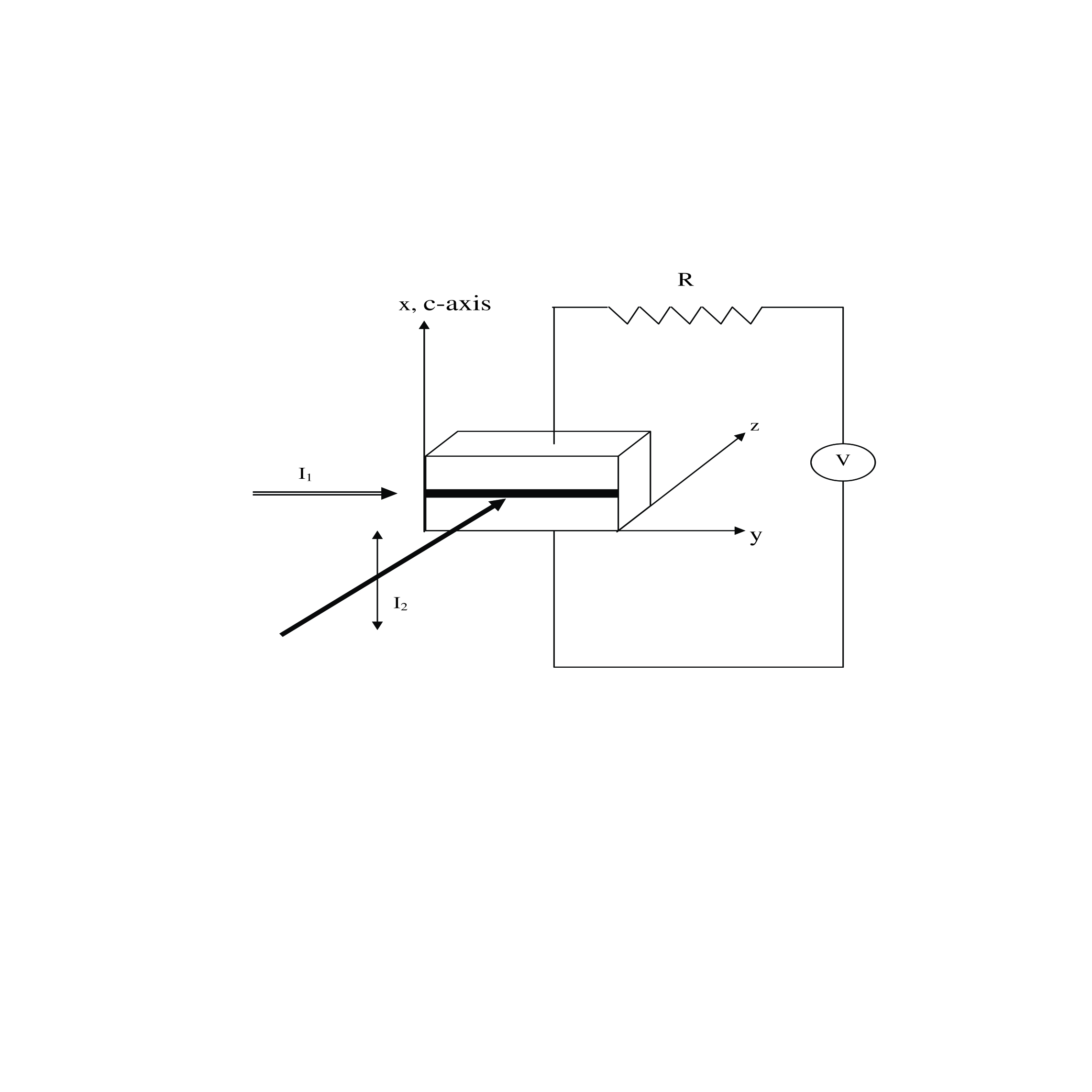
Figure 8: Optical configuration for two-photon photorefractive effect. The crystal is illuminated with a gating beam of constant intensity $I_{1}$.

In order to estimate the optical nonlinearity arising out in two photon-photorefractive media, we consider an optical configuration whose schematic diagram is shown in figure (8).

Insert Figure (8) here

The electrical circuit consist of a crystal ( could be made of photovoltaic-photorefractive or non photovoltaic-photorefractive material), external electric field bias voltage V and external resistance $R$. $V_{0}$ and $E_{0}$ respectively denote the potential and electric field strength between the crystal electrodes which are separated by a distance d. Assuming the spatial extent of optical wave is much less than d, we have $E_{0}=V_{0}/d$; additionally $V/d=E_{a}$.

Therefore,

$$V=E_{0}d+JSR=E_{a}d,$$ (46)

where $S$ is the surface area of the crystal electrodes and $J$ is the current density. The soliton forming optical beam with intensity $I_{2}$ propagates along the $z$ direction of the crystal and is permitted to diffract only along the $x$ direction. The optical beam is polarized along the $x$ axis which is also the direction of crystal c-axis and the external bias field is also directed along this direction. The crystal is illuminated with a gating beam of constant intensity $I_{1}$. The space charge field $E_{sc}$ due to two-photon photorefractive phenomenon can be obtained from the set of rate, current, and Poisson’s equations proposed by Castro-Camus et. al. [91]. In the steady state, these equations are

$$(s_{1}I_{1}+\beta_{1})(N_{D}-N_{D}^{+})-\gamma_{1}N_{i}N_{D}^{+}-\gamma_{R}NN_{D}^{+}=0,$$ (47)

$$(s_{1}I_{1}+\beta_{1})(N_{D}-N_{D}^{+})+\gamma_{2}N(N_{it}-N_{i})-\gamma_{1}N_{i}N_{D}^{+}-(s_{2}I_{2}+\beta_{2})N_{i}=0,$$ (48)

$$(s_{2}I_{2}+\beta_{2})N_{i}+\frac{1}{e}\frac{\partial J}{\partial x}-\gamma_{R}NN_{D}^{+}-\gamma_{2}N(N_{it}-N_{i})=0,$$ (49)

$$\epsilon_{0}\epsilon_{r}\frac{\partial E_{sc}}{\partial x}=e(N_{d}^{+}-N-N_{i}-N_{A}),$$ (50)

$$J=e\mu NE_{sc}+\kappa_{p}s_{2}(N_{D}-N_{D}^{+})I_{2}+eD\frac{\partial N}{\partial x},$$ (51)

$$\frac{\partial J}{\partial x}=0,\ \ \ \\ \\ \\ \\ J=constant,$$ (52)

where $N_{D}$ , $N_{D}^{+}$ , $N_{A}$ and $N$ are the donor density, ionized donor density, acceptor or trap density and density of electrons in the conduction band, respectively. $N_{i}$ is the density of electrons in the intermediate state, $N_{it}$ is the density of traps in the intermediate state. $\kappa_{p}$ , $\mu$ and $e$ are respectively the photovoltaic constant, electron mobility and electronic charge; $\gamma_{R}$ is the recombination factor of the conduction to valence band transition, $\gamma_{1}$ is the recombination factor for intermediate allowed level to valence band transition, $\gamma_{2}$ is the recombination factor of the conduction band to intermediate level transition; $\beta_{1}$ and $\beta_{2}$ are respectively the thermo-ionization probability constant for transitions from valence band to intermediate level and intermediate level to conduction band; $s_{1}$ and $s_{2}$ are photo-excitation crosses. $D$ is the diffusion coefficient and $I_{2}$ is the intensity of the soliton forming beam. We adopt the usual approximations $N_{D}^{+}\sim N_{A}$ and $N_{it}-N_{i}<<N_{A}$ . In addition, we also assume that, the power density is uniform at large distance from the center of the soliton forming beam, thus, at $x\rightarrow\pm\infty,\ I_{2}(x\rightarrow\pm\infty,z)=constant=I_{2\infty}$. Obviously, the space charge field in the above remote region is also uniform, i.e., $E_{sc}(x\rightarrow\pm\infty,z)=E_{0}$. The space charge field can be obtained using standard procedure [94], which turns out to be

$$E_{sc} = gE_{a}\frac{(I_{2\infty}+I_{2d})(I_{2}+I_{2d}+\frac{\gamma_{1}N_{A}}{s_{2}})}{(I_{2}+I_{2d})(I_{2\infty}+I_{2d}+\frac{\gamma_{1}N_{A}}{s_{2}})}$$ (53)

$${}+E_{p}\frac{s_{2}(gI_{2\infty}-I_{2})(I_{2}+I_{2d}+\frac{\gamma_{1}N_{A}}{s_{2}})}{(I_{2}+I_{2d})(s_{1}I_{1}+\beta_{1})}$$

$${}-\frac{D}{\mu s_{2}}\frac{\gamma_{1}N_{A}}{(I_{2}+I_{2d})(I_{2\infty}+I_{2d}+\frac{\gamma_{1}N_{A}}{s_{2}})}\frac{\partial I_{2}}{\partial x},$$

where $E_{p}=\kappa_{p}N_{A}\gamma_{R}/e\mu$ is the photovoltaic field, $I_{2d}=\beta_{2}/s_{2}$ is the so called dark irradiance. $g=1/(1+q)$, $q=\frac{e\mu N_{\infty}SR}{d}$ , $N_{\infty}=N(x\rightarrow\pm\infty)$. In general the parameter $g$ is a positive quantity and is bounded between $0\leq g\leq 1$. Under short circuit condition $R=0$ and $g=1$, implying that the external electric field is totally applied to the crystal. For open circuit condition $R\rightarrow\infty,$ thus, $g=0$ i.e., no bias field is applied to the crystal.

8.2 Nonlinear Evolution Equation

As usual, the optical field of the incident soliton forming beam is taken as $\overrightarrow{E}=\overrightarrow{x}\Phi(x,z)\exp[i(kz-\omega t)]$, where $k=k_{0}n_{e},k_{0}=2\pi/\lambda_{0}$, $\lambda_{0}$ is the free space wavelength of the optical field, $n_{e}$ is the unperturbed extraordinary index of refraction and $\Phi$ is the slowly varying envelope of the optical field. Employing the space charge field as given by equation(53) and following the procedure employed earlier, the nonlinear Schrödinger equation for the normalized envelope $A(s,\xi)$ can be obtained as [94]

$$i\frac{\partial A}{\partial\xi}+\frac{1}{2}\frac{\partial^{2}A}{\partial s^{2}}-\beta g\frac{(1+\rho)(1+\sigma+|A|^{2})A}{(1+|A|^{2})(1+\sigma+\rho)}- \alpha\eta\frac{(g\rho-|A|^{2})(1+\sigma+|A|^{2})A}{1+|A|^{2}}$$ (54)

$${}+\frac{\delta\sigma A}{(1+|A|^{2})(1+\sigma+|A|^{2})}\frac{\partial|A|^{2}}{\partial s}=0,$$

where $\rho=I_{2\infty}/I_{2d}$, $A=\sqrt{\frac{n_{e}}{2\eta_{0}I_{2d}}}\Phi$, $\xi=z/(k_{0}n_{e}x_{0}^{2})$, $s=x/x_{0}$, $\beta=(k_{0}x_{0})^{2}(n_{e}^{4}r_{33}/2)E_{a}$, $\alpha=(k_{0}x_{0})^{2}(n_{e}^{4}r_{33}/2)E_{p}$, $\delta=(k_{0}x_{0})^{2}(n_{e}^{4}r_{33}/2)D/(x_{0}\mu)$, $\eta=\beta_{2}/(s_{1}I_{1}+\beta_{1}),\sigma=\frac{\gamma_{1}N_{A}}{s_{2}I_{2d}}=\frac{\gamma_{1}N_{A}}{\beta_{2}}$ and $\eta_{0}=\sqrt{\mu_{0}/\epsilon_{0}}.\ r_{33}$ is the electro-optic coefficient of the two-photon photorefractive crystal. Equation(54) can be employed to investigate screening, photovoltaic and screening photovoltaic solitons under appropriate experimental configuration.

8.3 Screening Solitons

For screening solitons, the crystal should be nonphotovoltaic-photorefractive(i.e., $\alpha=0$). Assuming that the external bias field is totally applied to the crystal(R=0), thus, $E_{a}=E_{0}$ and $g=1$. Neglecting diffusion, the expression for space charge field $E_{sc}$ turns out to be [91, 92]

$$E_{sc}=E_{0}\frac{(I_{2\infty}+I_{2d})(I_{2}+I_{2d}+\frac{\gamma_{1}N_{A}}{s_{2}})}{(I_{2}+I_{2d})(I_{2\infty}+I_{2d}+\frac{\gamma_{1}N_{A}}{s_{2}})}.$$ (55)

Note that though the gating beam of constant intensity $I_{1}$ is required to maintain a quantity of excited electrons density in the intermediate allowed level, it does not appear in the expression of space charge field. The relevant modified nonlinear Schrödinger equation is obtained as

$$i\frac{\partial A}{\partial\xi}+\frac{1}{2}\frac{\partial^{2}A}{\partial s^{2}}-\beta\frac{(1+\rho)(1+\sigma+|A|^{2})A}{(1+|A|^{2})(1+\sigma+\rho)}=0.$$ (56)

Fundamental properties of dark, bright and grey solitary wave solutions of this equation have been investigated extensively by several authors [92, 96, 97, 98]. Self deflection of these solitons due to diffusion [92] and effects of higher order space charge field on self deflection have been also examined [97]. Jiang et. al. [98] have examined temporal behavior of these solitons. They predicted that, in the low amplitude regime, FWHM of solitons will decrease monotonically to a minimum steady state value, and that the transition time of such solitons should be independent of $\beta$ or soliton intensity and is close to $10T_{d}$, where $T_{d}$ is the dielectric relaxation time. They also predicted that the temporal properties of dark solitons are similar to those of the bright solitons.

 Intensity of bright solitons vanishes at infinity, thus, $I_{2\infty}=\rho=0$. Therefore,

$$i\frac{\partial A}{\partial\xi}+\frac{1}{2}\frac{\partial^{2}A}{\partial s^{2}}-\frac{\beta}{1+\sigma}\left(1+\frac{\sigma}{1+|A|^{2}}\right)A=0.$$ (57)

Assume a bright soliton of the form $A=p^{1/2}y(s)\exp(i\nu\xi)$, where $\nu$ is the nonlinear shift in propagation constant and $y(s)$ is a normalized real function, which is bounded as $0\leq y(s)\leq 1$. The parameter $p$ stands for the ratio of the peak intensity of the soliton to dark irradiance $I_{2d}$. The profile of the soliton turns [92] out to be

$$s=\pm\int_{y}^{1}\frac{[\frac{2\beta\sigma}{(1+\sigma)}]^{-1/2}p^{1/2}}{[\ln(1+p\widehat{y}^{2})-\widehat{y}^{2}\ln(1+p)]^{1/2}}d\widehat{y},$$ (58)

while the expression for nonlinear phase shift is given by

$$\nu=-\left(\frac{\beta}{1+\sigma}\right)[1+\frac{\sigma}{p}\ln(1+p)].$$ (59)

From equation(58), it can be easily shown that the bright soliton requires $\beta>0$ i.e., $E_{0}>0$. Therefore, screening bright spatial solitons can be formed in a two-photon photorefractive medium only when external bias field is applied in the same direction with respect to the optical c-axis. FWHM of these spatial solitons is inversely proportional to the square root of the absolute value of the external bias field. In the low amplitude limit i.e.,when $|A|^{2}<<1$, equation(57) reduces to

$$i\frac{\partial A}{\partial\xi}+\frac{1}{2}\frac{\partial^{2}A}{\partial s^{2}}-\frac{\beta}{1+\sigma}\left(1+\sigma-\sigma|A|^{2}\right)A=0.$$ (60)

Above equation can be exactly solved analytically and the one-soliton solution is

$$A(s,\xi)=p^{1/2}sech\left[\left(\frac{\beta p\sigma}{1+\sigma}\right)^{1/2}s\right]\\ exp\left[i\frac{\beta(p\sigma-2\sigma-2)}{2(1+\sigma)}\xi\right].$$ (61)

The spatial width ($\tau_{FWHM}$) of these solitons are $\tau_{FWHM}=2\ln(1+\sqrt{2})\left(\frac{1+\sigma}{p\sigma\beta}\right)^{1/2}$.

To obtain dark soliton solution, we take $A(s,\xi)=\rho^{1/2}y(s)\exp[i\mu\xi]$, where $y(s)$ is a normalized odd function of s and satisfies the following boundary conditions: $y(s=0)=0$, $y(s\rightarrow\pm\infty)=1$, and all the derivatives of $y(s)$ vanish at infinity. The profile $y(s)$ of these solitons can be obtained [92] using the following relationship

$$s=\pm\int_{y}^{0}\frac{[\frac{-2\beta\sigma}{(1+\sigma+\rho)}]^{-1/2}}{\left[(\widehat{y}^{2}-1)-\frac{(1+\rho)}{\rho}\ln\left(\frac{1+\rho\widehat{y}^{2}}{1+\rho}\right)\right]^{1/2}}d\widehat{y},$$ (62)

and the nonlinear phase shift $\mu=-\beta$. The dark solitons require $\beta<0$. In the low amplitude limit i.e., when $|A|^{2}<<1$,  equation(56) reduces to

$$i\frac{\partial A}{\partial\xi}+\frac{1}{2}\frac{\partial^{2}A}{\partial s^{2}}-\frac{\beta(1+\rho)}{(1+\sigma+\rho)}(1+\sigma-\sigma|A|^{2})A=0.$$ (63)

The dark soliton solution of above equation turns out to be

$$A(s,\xi)=\rho^{1/2}\tanh\left[-\left(\frac{\beta\rho\sigma}{1+\sigma+\rho}\right)^{1/2}s\right]exp\left[\frac{i\beta(1+\rho)(\rho\sigma-\sigma-1)\xi}{1+\sigma+\rho}\right].$$ (64)

The spatial width ( $\tau_{FWHM}$) of these solitons are $\tau_{FWHM}=2\ln(1+\sqrt{2})\left(\frac{1+\rho+\sigma}{-\rho\sigma\beta}\right)^{1/2}$. Rare earth doped strontium barium niobate (SBN) could be a good candidate for observing these solitons, since, they have an intermediate level for the two step excitation. In addition to bright and dark solitons, equation(56) also predict steady state gray solitons under appropriate bias condition. These screening gray solitons were investigated by Zhang et. al. [96]. Properties of these gray solitons are similar to fundamental properties of one-photon photorefractive gray spatial solitons. For example, they require bias field in opposite to the optical c-axis of the medium and their FWHM is inversely proportional to the square root of the absolute value of the bias field. The main difference between one-photon and two-photon gray solitons is that one-photon gray solitons rely on one-photon photorefractive phenomenon to set up space charge field, while the two-photon photorefractive gray solitons rely on two-photon photorefractive phenomenon to set up space charge field.

8.4 Photovoltaic Solitons

We consider a photovoltaic photorefractive crystal under open circuit condition ($R=0$, $g=0$), the expression for space charge field from equation(53) reduces to

$$E_{sc}=-E_{p}\frac{s_{2}I_{2}(I_{2}+I_{2d}+\frac{\gamma_{1}N_{A}}{s_{2}})}{(I_{2}+I_{2d})(I_{1}s_{1}+\beta_{1})}-\frac{D}{\mu s_{2}}\frac{\gamma_{1}N_{A}}{(I_{2}+I_{2d})\left(I_{2\infty}+I_{2d}+\frac{\gamma_{1}N_{A}}{s_{2}}\right)}\frac{\partial I_{2}}{\partial x}.$$ (65)

Upon neglecting diffusion, the nonlinear Schrödinger equation for the normalized envelope $A(s,\xi)$ can be obtained as

$$i\frac{\partial A}{\partial\xi}+\frac{1}{2}\frac{\partial^{2}A}{\partial s^{2}}+\alpha\eta\frac{(1+\sigma+|A|^{2})|A|^{2}}{(1+|A|^{2})}A=0.$$ (66)

Bright, dark and gray photovoltaic solitons of equation(66) have been examined by several authors [93, 100]. Deflection of these solitons and higher order effects have been also given adequate attention [93, 100]. For bright solitons, we consider a similar profile as it was considered for screening solitons, and, the profile of such solitons turns out to be [93, 100]

$$s=\pm(\alpha\eta)^{-1/2}\int_{y}^{1}\left\{\frac{2\sigma}{p}[\ln(1+p\widehat{y}^{2})-\widehat{y}^{2}\ln(1+p)]+p\widehat{y}^{2}(1-p\widehat{y}^{2})\right\}^{-1/2}d\widehat{y},$$ (67)

where the nonlinear phase shift is given by

$$\nu=\alpha\eta\sigma[1-\frac{1}{p}\ln(1+p)]+\frac{\alpha\eta p}{2}.$$ (68)

The bright soliton requires $\alpha>0,i.e.,E_{p}>0$, thus the photovoltaic field should be in the same direction with respect to the optical c-axis of the medium. In the low amplitude limit ($|A|^{2}<<1$), FWHM of these solitons are inversely proportional to the square root of the absolute value of the photovoltaic field.


The profile of dark photovoltaic solitons, following a similar procedure, turns out to be [93]

$$s=\pm(-\alpha\eta)^{-1/2}\int_{y}^{0}\left[\frac{2\sigma}{1+\rho}(\widehat{y^{2}}-1)-\frac{2\sigma}{\rho}\ln\left(\frac{1+\rho\widehat{y}^{2}}{1+\rho}\right)+\rho(\widehat{y}^{2}-1)^{2}\right]^{-1/2}d\widehat{y},$$ (69)

and the nonlinear phase shift is given by

$$\mu=\alpha\eta\rho\left(1+\frac{\sigma}{1+\rho}\right).$$ (70)

The two-photon photovoltaic solitons require a separate gating beam to produce a quantity of excited electrons from the valance band to the intermediate level of the material. Without the gating beam, the signal beam cannot evolve into a spatial soliton. By adjusting the gating beam, one can control the width as well as formation of two-photon photovoltaic solitons.

8.5 Screening Photovoltaic Solitons

Steady state screening photovoltaic solitons are obtainable when an electric field is applied to a photovoltaic photorefractive crystal. These SP solitons result from both the photovoltaic effect and spatially nonuniform screening of the applied field. Recently, bright and dark screening photovoltaic (SP) solitons have been investigated by Zhang and Liu [94]. The normalized bright field profile $y(s)$ of these solitons can be determined ( with  $\delta=0$) from equation(54), which turns out to be [94]:

$$s = \pm\int_{y}^{1}\{\frac{2g\beta\sigma}{p(1+\sigma)}[\ln(1+p\widehat{y}^{2})-\widehat{y}^{2}\ln(1+p)]$$ (71)

$${}+\frac{2\alpha\eta\sigma}{p}[\ln(1+p\widehat{y}^{2})-\widehat{y}^{2}\ln(1+p)]+\alpha\eta p\widehat{y}^{2}(1-\widehat{y}^{2})\}^{-1/2}d\widehat{y}.$$

The nonlinear phase shift $\nu$ of these solitons is given by

$$\nu=-\frac{g\beta}{1+\sigma}[1+\frac{\sigma}{p}\ln(1+p)]+\alpha\eta\sigma[1-\frac{1}{p}\ln(1+p)]+\frac{\alpha\eta p}{2}.$$ (72)

Please note that unlike bright screening solitons, in the present case, it is not necessary that the value of $\beta$ should be positive. However, the sign of $\alpha$ and $\beta$ should be such that the curly bracketed term in equation(71) is positive. From equation(54) the normalized dark field profile y(s) can be obtained as [94]:

$$s = \pm\int_{y}^{0}\{-\frac{2g\beta\sigma}{(1+\rho+\sigma)}[(\widehat{y}^{2}-1)$$ (73)

$${}-\frac{1+\rho}{\rho}\ln\left(\frac{1+\rho\widehat{y}^{2}}{(1+\rho)}\right)]-\alpha\eta[\frac{2\sigma(1+g\rho)}{1+\rho}(\widehat{y}^{2}-1)$$

$${}-\frac{2\sigma(1+g\rho)}{\rho}\ln\left(\frac{1+\rho\widehat{y}^{2}}{1+\rho}\right)+\rho(\widehat{y}^{2}-1)^{2}]\}^{-1/2}d\widehat{y},$$

where the nonlinear phase shift is given by

$$\mu=-g\beta+\alpha\eta\rho(1-g)\left(1+\frac{\sigma}{1+\rho}\right).$$ (74)

By setting $\alpha=0$ and $g=1$ in equation(71), we recover bright solitons of equation(58). Similarly, by setting $\alpha=0$ and $g=1$ in equation(73), we recover dark solitons of equation(62). In addition, by taking $\beta=0$ and $g=0$ in equation(71) i.e., in open circuit realization, we recover bright PV solitons of equation(67). Similarly, by setting $g=0$ and $\beta=0$, we recover dark PV solitons of equation(69) from equation(73).

As pointed out by Zhang and Liu [94], these two-photon SP solitons may be considered as the unity form of two-photon screening and two-photon photovoltaic solitons under open circuit realization. If the biased field is much stronger in comparison to the photovoltaic field, then the screening photovoltaic solitons are just like screening solitons. If the applied field is absent, the screening photovoltaic solitons degenerate into the photovoltaic solitons in the open circuit condition$(\beta=0,g=0)$. In other words, the open circuit photovoltaic solitons or screening solitons are special cases of the screening photovoltaic solitons. Equation(73) also predicts the existence of two-photon photovoltaic solitons when $g=1$ and $\beta=0$ i.e., two-photon photovoltaic solitons in closed circuit realization.
 Before closing this section, a brief comment on gray two-photon screening PV solitons in biased two-photon phototvoltaic crystals seems inevitable. Equation(54) predicts the existence of such solitons [102]. The properties of these gray solitons, such as, their normalized intensity profiles, intensity FWHM, transverse velocity and transverse phase profiles have been discussed in detail by Zhang et. al. [102]. They become narrower as the grayness parameter m decreases for a given normalized intensity ratio $\rho$. However, the soliton width generally decreases and transverse velocity generally increases with intensity ratio $\rho$. In addition, soliton phase varies in a very involved fashion across transverse direction and the total phase jump of these solitons exceeds $\pi$ for relatively low value of the grayness parameter $m$.

9 Vector Solitons

Thus far, we have discussed optical spatial solitons which are solutions of a single NLS equation. These solutions are due to a single optical beam with a specific polarization and the polarization is maintained during propagation. However, always this specific picture may not hold good. Two or more optical beams may be mutually trapped and depend on each other in such a way that each of them propagates undistorted. Thus, several field components at different or same frequencies or polarizations may interact and yield shape preserving propagation. In order to discuss such cases, we need to solve a set of coupled NLS equations. Shape preserving solutions of this set of coupled NLS equations are called vector solitons. Only in specific cases, the constituents of these solitons are vector fields associated with solitons. In general, they are multi component in nature.

9.1 Two Component Incoherently Coupled Vector Solitons

Among spatial solitons interaction, pairing of two spatial solitons has been always an intriguing and extensively investigated issue. When two such soliton forming beams propagate, they interact through cross phase modulation (XPM) and induce a refractive-index modulation created by both beams. Two beams are mutually trapped and depend on each other in such a way that each of them propagates undistorted. Very recently, vector screening solitons [104, 105, 106, 107] have been investigated, that involve two polarization components of an optical beam which are orthogonal to each other. Depending on the symmetry class of the crystal and its orientation, these solitary beams obey cross or self coupled vector systems of dynamical equations.
 A new type of steady state incoherently coupled soliton pair was discovered in biased photorefractive crystals [108], which exists only when the two soliton forming beams possess same polarization and frequency and are mutually incoherent [108, 109, 110, 111, 112, 113, 114, 115, 116, 117, 118, 119, 120, 121, 122, 123] . These solitons can propagate in bright-bright, dark-dark, bright-dark and gray-gray configurations, and they can be realized in simple experimental arrangement with two mutually incoherent collinearly propagating optical beams. Since two beams are mutually incoherent, no phase matching is required and they experience equal effective electro-optic coefficients. The idea of two incoherently coupled solitons has been generalized and extended to soliton families where number of constituent solitons are more than two. Such incoherently coupled families can be established provided they have same polarization, wavelength and are mutually incoherent. Bright-bright, dark-dark [118], bright-dark [119, 120, 121] as well as gray-gray [113] configurations have been investigated. These multi component solitons are stable. In next few sections, we confine our discussion on two component spatial photorefractive vector solitons which are co-propagating and overlapping.

9.1.1 Coupled Solitary Wave Equations Due to Single Photon Phenomenon

To start with, we consider a pair of optical beams which are propagating in a photorefractive crystal ( the crystal could be PV-PR or non PV-PR) along z-direction. They are of same frequency and mutually incoherent. The optical c-axis of the crystal is oriented along the x direction. The polarization of both beams is assumed to be parallel to the x-axis. These two optical beams are allowed to diffract only along the x-direction and y-dynamics has been implicitly omitted in the analysis. For the sake of simplicity the photorefractive material is assumed to be lossless. The perturbed refractive index along the x-axis is given by $\widehat{n}_{e}^{2}=n_{e}^{2}-n_{e}^{4}r_{33}E_{sc}$. The optical fields are expressed in the form $\overrightarrow{E_{1}}=\overrightarrow{x}\Phi_{1}(x,z)\exp(ikz)$ and $\overrightarrow{E_{2}}=\overrightarrow{x}\Phi_{2}(x,z)\exp(ikz)$, where $\Phi_{1}$ and $\Phi_{2}$ are slowly varying envelopes of two optical fields, respectively. It can be readily shown that the slowly varying envelopes of two interacting spatial solitons inside the photovoltaic PR crystal are governed by the following evolution equations:

$$i\frac{\partial\Phi_{1}}{\partial z}+\frac{1}{2k}\frac{\partial^{2}\Phi_{1}}{\partial x^{2}}-\frac{k_{0}n_{e}^{3}r_{33}E_{sc}}{2}\Phi_{1}=0,$$ (75)

$$i\frac{\partial\Phi_{2}}{\partial z}+\frac{1}{2k}\frac{\partial^{2}\Phi_{2}}{\partial x^{2}}-\frac{k_{0}n_{e}^{3}r_{33}E_{sc}}{2}\Phi_{2}=0.$$ (76)

For relatively broad optical beams and under strong bias condition, the space charge field can be obtained from equation(11) as

$$E_{sc}=E_{0}\frac{I_{\infty}+I_{d}}{I+I_{d}}+E_{P}\frac{I_{\infty}-I}{I+I_{d}},$$ (77)

where in the present case $I=I(x,z)$ is total power density of two optical beams, $I_{\infty}$ is the total power density of soliton pair at a distance far away from the center of the crystal i.e., $I_{\infty}=I(x\rightarrow\pm\infty)$. $E_{0}$ is the value of the space charge field at far away from the beam center i.e., $x\rightarrow\pm\infty$. For two mutually incoherent beams, total optical power density I can be written as $I(x,z)=n_{e}/(2\eta_{0})(|\Phi_{1}|^{2}+|\Phi_{2}|^{2})$ i.e., sum of Poynting fluxes. Substituting the expression of $E_{sc}$ in equations(75) and (76), we derive the following dimensionless dynamical equations for two soliton forming optical beams:

$$i\frac{\partial A_{j}}{\partial\xi}+\frac{1}{2}\frac{\partial^{2}A_{j}}{\partial s^{2}}-\beta(1+\rho)\frac{A_{j}}{(1+|A_{j}|^{2}+|A_{3-j}|^{2})}-\alpha\frac{(\rho-|A_{j}|^{2}-|A_{3-j}|^{2})A_{j}}{(1+|A_{j}|^{2}+|A_{3-j}|^{2})}=0,\ \ \ \ \j=1,2\ ,\$$ (78)

where $\beta=(k_{0}x_{0})^{2}(n_{e}^{4}r_{33}/2)E_{0}$ , $\alpha=(k_{0}x_{0})^{2}(n_{e}^{4}r_{33}/2)E_{p}$, $A_{j}=\sqrt{\frac{n_{e}}{2\eta_{0}I_{d}}}\Phi_{j}$; $\xi$, $s$ and $\rho$ are defined earlier. Above set of two coupled Schrödinger equations can be examined for bright-bright, bright-dark, dark-dark, gray-gray screening, photovoltaic as well as screening photovoltaic solitons [110, 111, 112, 113, 114, 115, 116, 117, 118, 119, 120]. It can be easily shown that when the total intensity of the two coupled solitons is much lower than the effective dark irradiance, the coupled soliton equations reduce to Manakov equations. The dark-dark, bright-bright and dark-bright soliton pair solutions of these Manakov equations can be obtained under appropriate bias and photovoltaic fields [117].
 With the growing applications of self focusing and spatial solitons in modern technology, several mathematical methods have evolved to address soliton dynamics [124, 125, 126, 127, 128, 129]. In particular, Christodoulides et. al. [108] have developed a very efficient method to numerically solve a set of coupled equations which has been employed extensively to investigate coupled solitons in PR media. In this method, two coupled equations are converted to one ordinary differential equation which is then numerically solved to obtain soliton profiles. The main difficulty with this method is its inability to capture the existence of a large family of stable stationary solitons. We will discuss more on this in the latter part of the article. What follows in the next section is a discussion on incoherently coupled solitons employing the method of reference 108.

9.2 Incoherently Coupled Screening Vector Solitons

In this section we consider incoherently coupled bright-bright, dark-dark as well as bright-dark screening solitons in a biased nonphotovoltaic photorefractive crystal. These coupled solitons were identified by Christodoulides et. al. [108]. The parameter $\alpha=0$, since, the crystal is nonphotovoltaic, hence, relevant coupled Schrödinger equations are as follows

$$i\frac{\partial A_{j}}{\partial\xi}+\frac{1}{2}\frac{\partial^{2}A_{j}}{\partial s^{2}}-\beta(1+\rho)\frac{A_{j}}{(1+|A_{j}|^{2}+|A_{3-j}|^{2})}=0,$$ (79)

We first consider a bright-bright soliton pair for which $I_{\infty}=\rho=0$. Expressing stationary soliton solutions of the form $A_{1}=p^{1/2}y(s)\cos\theta\ \exp(i\mu\xi)$ and $A_{2}=p^{1/2}y(s)\sin\theta\ \exp(i\mu\xi)$, where $\mu$ represents nonlinear shift of the propagation constant, and y(s) is a normalized real function between $0\leq y(s)\leq 1$. The parameter $\theta$ is an arbitrary projection angle which ultimately decides the relative power of two components. Substituting $A_{1}$ and $A_{2}$ in equation(79), we get the following ordinary differential equation

$$\frac{d^{2}y}{ds^{2}}-2\mu y-2\beta\frac{y}{1+py^{2}}=0,$$ (80)

and

$$\mu=-(\frac{\beta}{p})\ln(1+p).$$ (81)

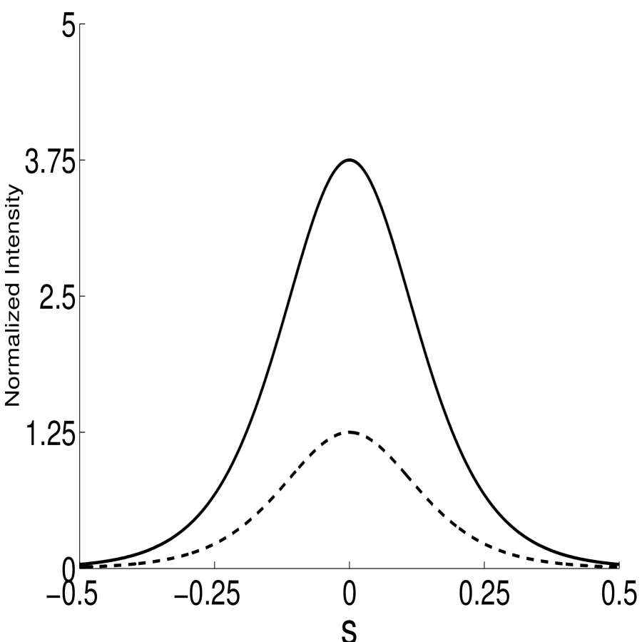
Figure 9: Components of a bright-bright soliton pair. $\beta=43,p=5$ and $\theta=30^{0}$.

Earlier in section (7.3), it was shown that, above equation admits bright solitons when $\beta$  i.e., $E_{0}$ is positive. The, same condition holds good for bright-bright pair which can be obtained by numerically solving equation (80). A typical bright-bright pair has been depicted in figure (9).

Insert Figure (9) here

For dark-dark pairs, $I_{\infty}$ and $\rho$ are finite. We express $A_{1}$ and $A_{2}$ as $A_{1}=\rho^{1/2}y(s)\cos\theta\exp(i\mu\xi)$ and $A_{2}=\rho^{1/2}y(s)\sin\theta\exp(i\mu\xi)$, with $|y(s)|\leq 1$. Thus, we have

$$\frac{d^{2}y}{ds^{2}}-2\mu y-2\beta(1+\rho)\frac{y}{1+\rho y^{2}}=0,$$ (82)

and

$$\mu=-\beta.$$ (83)

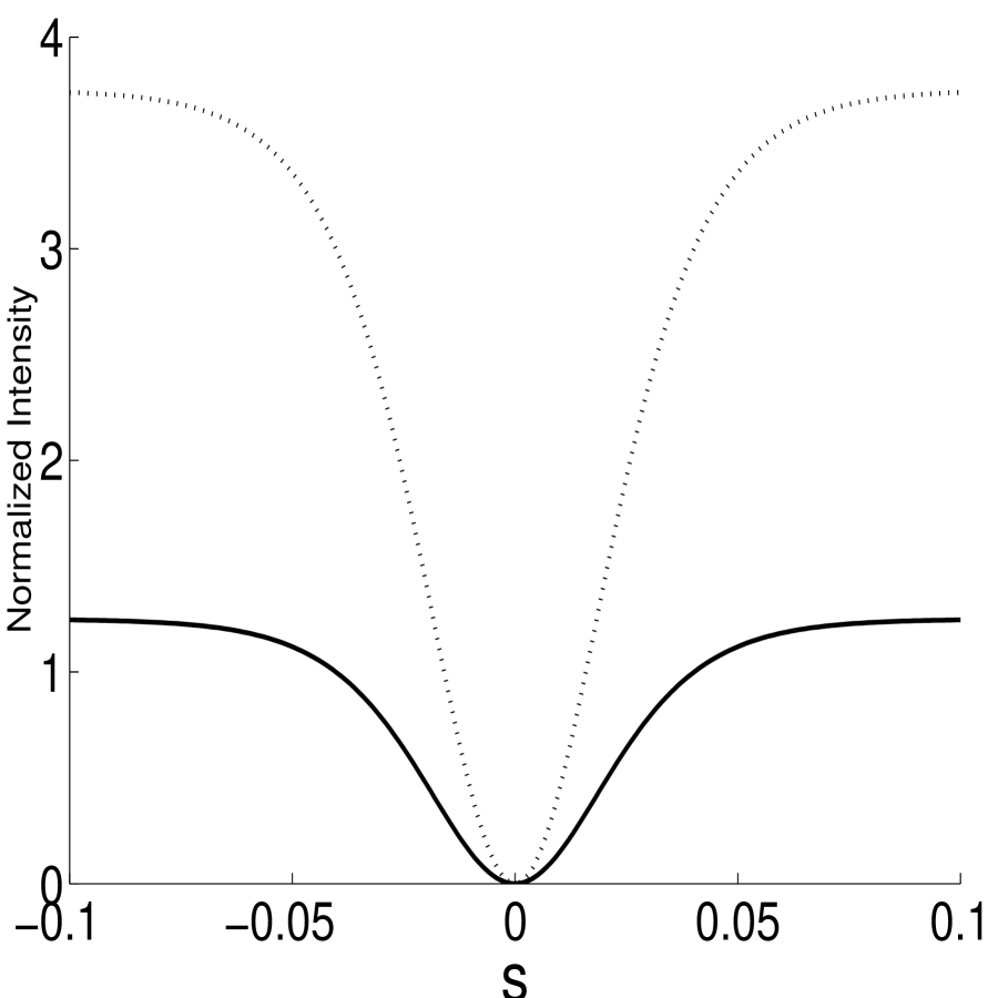
Figure 10: Components of a dark-dark soliton pair. $\beta=-43,\rho=5$ and $\theta=30^{0}$.

Equation (82) can be solved for dark-dark soliton pairs provided $\beta$  i.e., $E_{0}$ is negative. A typical dark-dark pair has been depicted in figure (10).

Insert Figure (10) here

For bright-dark soliton pair, we express $A_{1}$ and $A_{2}$ as $A_{1}=p^{1/2}f(s)\exp(i\mu\xi)$ and $A_{2}=\rho^{1/2}g(s)\exp(i\nu\xi)$, where $f(s)$ and $g(s)$ respectively represents envelope of bright and dark beams. Two positive quantities $p$ and $\rho$ represent the ratios of their maximum power density with respect to the dark irradiance $I_{d}$. Therefore, bright-dark soliton pair obeys following coupled ordinary differential equations:

$$\frac{d^{2}f}{ds^{2}}-2\left[\mu+\frac{\beta(1+\rho)}{1+pf^{2}+\rho g^{2}}\right]f=0,$$ (84)

and

$$\frac{d^{2}g}{ds^{2}}-2\left[\nu+\frac{\beta(1+\rho)}{1+pf^{2}+\rho g^{2}}\right]g=0.$$ (85)

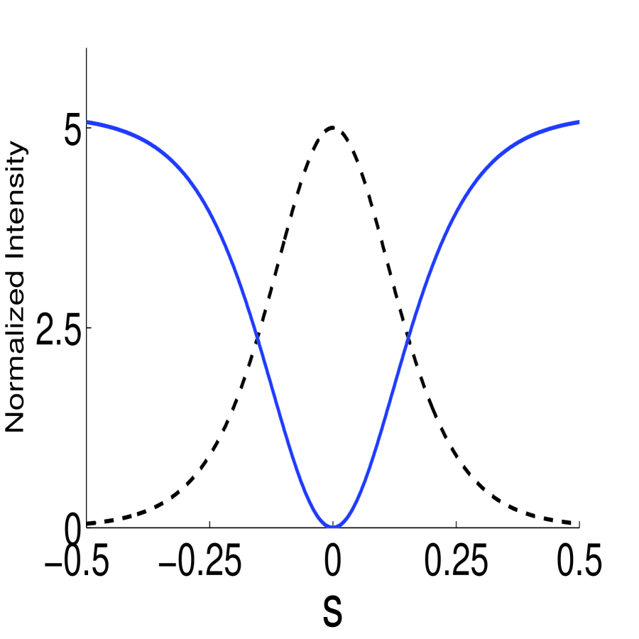
Figure 11: Components of a bright-dark soliton pair. $\beta=-43,\rho=5,\Lambda=-0.01$ and $\theta=30^{0}$.

A particular solution of above equations can be obtained using the simplification $f^{2}+g^{2}=1$. Employing appropriate boundary conditions, the nonlinear phase shifts $\mu$ and $\nu$ are obtained as: $\mu=-\frac{\beta}{\Lambda}\ln(1+\Lambda)$ and $\nu=-\beta$, where $\Lambda=(p-\rho)/(1+\rho)$. When peak intensities of two solitons are approximately equal, $\Lambda<<1$ . The approximate soliton solution [105, 108] in this particular case is given by $A_{1}=p^{1/2}\ sech[(\beta\Lambda)^{1/2}s]\exp[-i\beta(1-\Lambda/2)\xi],$ and $A_{2}=\rho^{1/2}\tanh[(\beta\Lambda)^{1/2}s]\exp[-i\beta\xi].$  These two soliton solutions are possible only when the product $(\beta\Lambda)$ is a positive quantity. A typical bright dark soliton pair is depicted in figure (11).

Insert Figure (11) here

9.2.1 Missing Bright Screening PV Solitons

In the preceeding section, we have followed the procedure developed in reference 108 and assumed a particular type of ansatz for the bright-bright pair. According to this method, the normalized power $P_{1}$ and $P_{2}$ of two solitons of the bright-bright pair are $P_{1}=p\sin^{2}\theta$ and $P_{2}=p\cos^{2}\theta$. Therefore, for a given $P_{1}$, $\theta$ has a fixed value, hence, the power of the other component has only one possible value which is unique. Or in other words a composite soliton can exist only with a single power ratio. In this section, we will show that for a given power of one component, the other component can exist with different power. Thus, the method of reference [108] fails to identify a large number of bright-bright solitons in a two component configuration. Therefore, our goal, in this section, is to demonstrate the existence of a new very large family of two-component composite screening photovoltaic spatial solitons in biased photovoltaic-photorefractive crystals which were not identified by the method of reference 108. For bright solitons, $\rho=0$, hence, relevant coupled equations for bright-bright screening PV solitons in biased PV-PR crystals [64] are

$$i\frac{\partial A_{j}}{\partial\xi}+\frac{1}{2}\frac{\partial^{2}A_{j}}{\partial s^{2}}+\frac{[\alpha(|A_{j}|^{2}+|A_{3-j}|^{2})-\beta]A_{j}}{(1+|A_{j}|^{2}+|A_{3-j}|^{2})}=0,$$ (86)

In order to analyze the behavior of these coupled solitons, we assume solutions of the form

$$A_{j}(s,\xi)=\Psi_{j}(s,\xi)\exp(-i\Omega_{j}\xi),$$ (87)

By virtue of use of equation(87) in equation (86), we obtain following equations:

$$\frac{\partial\Omega_{j}}{\partial\xi}\Psi_{j}-\frac{1}{2}\left(\frac{\partial\Omega_{j}}{\partial s}\right)^{2}\Psi_{j}+\frac{1}{2}\frac{\partial^{2}\Psi_{j}}{\partial s^{2}}+\alpha\Pi\Psi_{j}=0,$$ (88)

$$\frac{\partial\Psi_{j}}{\partial\xi}-\frac{\partial\Omega_{j}}{\partial s}\frac{\partial\Psi_{j}}{\partial s}-\frac{1}{2}\frac{\partial^{2}\Omega_{j}}{\partial s^{2}}\Psi_{j}=0,$$ (89)

where  $\Pi=\frac{\alpha(|\Psi_{1}|^{2}+|\Psi_{2}|^{2})-\beta}{1+|\Psi_{1}|^{2}+|\Psi_{2}|^{2}}$.  The last three terms of (88) determine the behavior of the eikonal $\Omega_{j}$ i.e., the convergence or divergence of two optical beams. The fourth term in this equation represents nonlinear refraction while the third term determines diffraction. Equation (89) determines the evolution of the beam envelope $\Psi_{j}$. In equation (88), $\Pi$ represents the contribution from nonuniform screening of the applied electric field and photovoltaic properties of the crystal as well.

Lowest order localized bright solitons, for which light is confined in the central region of the soliton, obey $\Psi_{j}(s=0)=\Psi_{jmax}$ and $\Psi_{j}=0$ as $s\rightarrow\pm\infty.$ The fundamental solutions of coupled Schrödinger equations, in a self focusing Kerr medium, are represented by sech functions. Equation (86) is a modified nonlinear Schrödinger equation(MNLSE) in saturating media. Due to the saturating nature of the medium, it is expected that the fundamental soliton solutions will not be exactly sech function. However, in many nonlinear optical problems involving NLSE and MNLSE in Kerr, cubic quintic, nonlocal and saturating media, approximate solutions have been obtained using Gaussian  [130, 131, 132, 133, 134, 135] or super Gaussian ansatz [135]. The motivation of employing such ansatz is two fold. Firstly, particularly true for Gaussian ansatz, mathematical formulations become easy. Secondly, numerically computed exact solutions are not widely different from Gaussian profiles in many cases. Thus, though approximate, Gaussian profile still provides good approximation to the problem. Hence, the solutions of above equations are taken to be Gaussian with amplitude and phase of the following form

$$\Psi_{j}(s,\xi)=\frac{\Psi_{j0}}{\sqrt{f_{j}(\xi)}}exp\left[-\frac{s^{2}}{2r_{j}^{2}(\xi)f_{j}^{2}(\xi)}\right],$$ (90)

$$\Omega_{j}(s,\xi)=\frac{s^{2}}{2}\beta_{j}(\xi)+\phi_{j}(\xi),$$ (91)

and

$$\beta_{j}(\xi)=-\frac{1}{f_{j}}\frac{df_{j}(\xi)}{d\xi},\ \ \ \$$ (92)

where, $\Psi_{jo}$ represents the peak power of the component of bright-bright solitons, $r_{j}$ is a positive constant, $f_{j}(\xi)$ is variable spatial width parameter; $r_{j}f_{j}(\xi)$ is the spatial width of these solitons and $\phi_{j}(\xi)$ is an arbitrary phase function. For a pair of nondiverging solitons at $\xi=0$, we should have $f_{j}=1$ and $\frac{df_{j}}{d\xi}=0$. Substituting for $\Psi_{j}$ and $\Omega_{j}$ in (88), using paraxial ray approximation [86, 126, 127] and equating coefficients of $s^{2}$ from both sides of (88), we obtain

$$\frac{d^{2}f_{j}}{d\xi^{2}}=\frac{1}{r_{j}^{4}f_{j}^{3}}-C\left(\frac{P_{j}}{r_{j}^{2}f_{j}^{2}}+\frac{P_{3-j}}{r_{3-j}^{2}f_{3-j}^{3}}\right)\frac{1}{\left(1+\frac{P_{j}}{f_{j}}+\frac{P_{3-j}}{f_{3-j}}\right)^{2}},$$ (93)

where $P_{j}=\Psi_{j0}^{2}$ and $C=2(\alpha+\beta)$. The solutions of above equation should give stationary and non-stationary coupled solitons of (86) for given set of power and spatial width.

9.2.2 Stationary Composite Solitons

In order to identify stationary composite solitons, we need to locate equilibrium points. The equilibrium points of equation(93) can be obtained from following equations

$$\frac{1}{r_{1}^{4}}-C\left(\frac{P_{1}}{r_{1}^{2}}+\frac{P_{2}}{r_{2}^{2}}\right)\frac{1}{\left(1+P_{1}+P_{2}\right)^{2}}=0,$$ (94)

and

$$\frac{1}{r_{2}^{4}}-C\left(\frac{P_{1}}{r_{1}^{2}}+\frac{P_{2}}{r_{2}^{2}}\right)\frac{1}{\left(1+P_{1}+P_{2}\right)^{2}}=0.$$ (95)

From above equations, it is obvious that $r_{1}=r_{2}=r$ is the condition for existence of stationary coupled solitons, where $r$ is a constant. Therefore, composite solitons with different spatial widths cannot propagate as a stationary entity. The existence equation of coupled solitons turns out to be

$$Cr^{2}=\frac{(1+P_{1}+P_{2})^{2}}{P_{1}+P_{2}}.$$ (96)

Obviously, for a bright-bright pair $C$ should be positive. From the existence equation, it is evident that though spatial widths of each of the two components are equal, their respective peak power can have different value. Equation (96) is equivalent to a quadratic equation in $P_{1}$, the root of which is obtained as

$$P_{1}=\left[(Cr^{2}-2P_{2}-2)\pm\sqrt{(Cr^{2}-2P_{2}-2)^{2}-4(P_{2}^{2}+2P_{2}+1-Cr^{2}P_{2})}\right]/2.$$ (97)

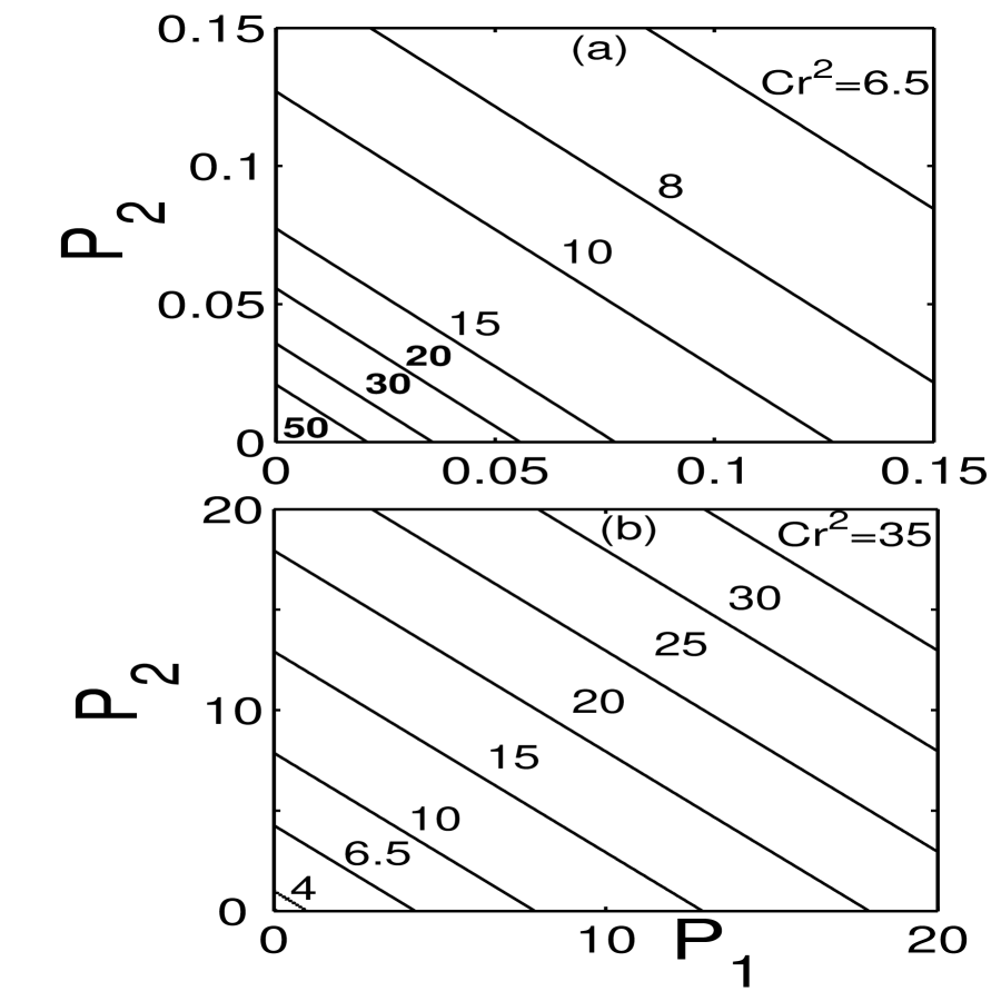
Figure 12: Existence curve of screening photovoltaic solitons. (a) Low power, (b) High power.

$P_{1}$ and $P_{2}$ are real and positive, hence, always $Cr^{2}\geq 4$ . For a given value of $C$, this relationship dictates a minimum width for the propagating soliton pair. The variation of $P_{1}$ with $P_{2}$ for different values of $r$ has been depicted in figure 12(a)-(b). Each point on any curve of these figures represents a stationary composite soliton with a definite spatial width and peak power.

Insert Figure (12) here

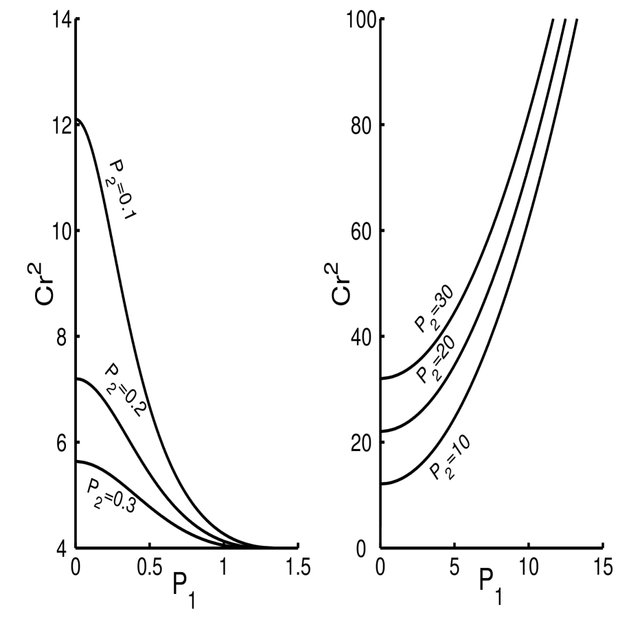
Figure 13: Variation of peak power $P_{1}$ of one of the component of the composite soliton with spatial width $r$ while the peak power of other component $P_{2}$ is constant.

An important issue is, whether for a given peak power of one of the component, the other component exists with only one or multiple values of peak power. This issue can be settled from figure (13) which shows the variation of width with peak power of one component keeping peak power of other component constant. It is evident from the figure that $P_{1}$ has a range of values for a fixed $P_{2}$, thus, with fixed $P_{2}$ other component can exist with different values of $P_{1}$. At this stage it is worth pointing out that these solitons cannot be identified with the method employed in ref. 108.

Insert Figure (13) here

9.2.3 Degenerate Bright Screening PV Bistable Solitons

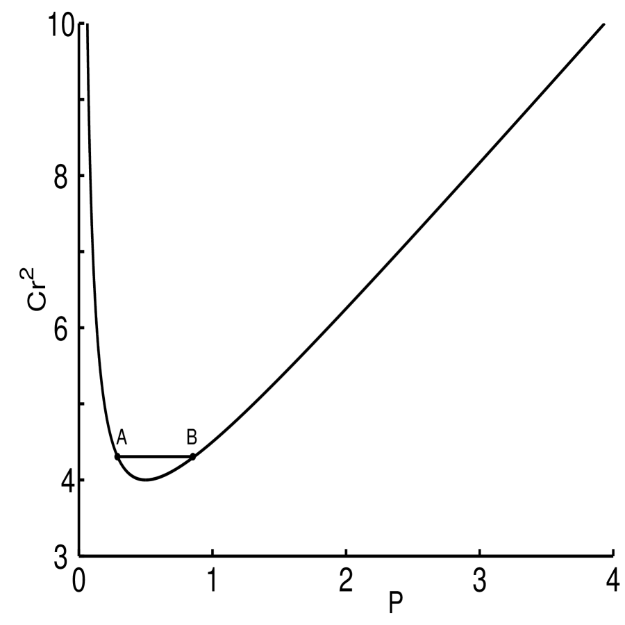
Figure 14: Variation of peak power $P$ of the degenerate composite soliton with spatial width $r$. Nature of the curve signifies existence of bistable property of solitons.

We take up a degenerate case in which peak power of two components is same and having same spatial width. Setting $P_{1}=P_{2}=P$ in (97), we obtain a quadratic equation of P, the solution of which is obtained as $P=[Cr^{2}-2\pm\sqrt{(Cr^{2}-4)^{2}-4]}/4$ , which implies that spatial width $r$ of each component of the composite soliton should be greater than $2/\sqrt{C}$, i.e., a two-component composite soliton whose individual spatial width is less than above value cannot propagate as a self trapped mode. In figure (14) we have displayed variation of $r$ with peak power $P$. From figure, existence of a bistable regime [66] is evident i.e., two sets of soliton pairs exist with same spatial width but having different peak power and consequently different peak amplitude. Only this degenerate case possesses bistable property.

Insert Figure (14) here

9.2.4 Numerical Simulation

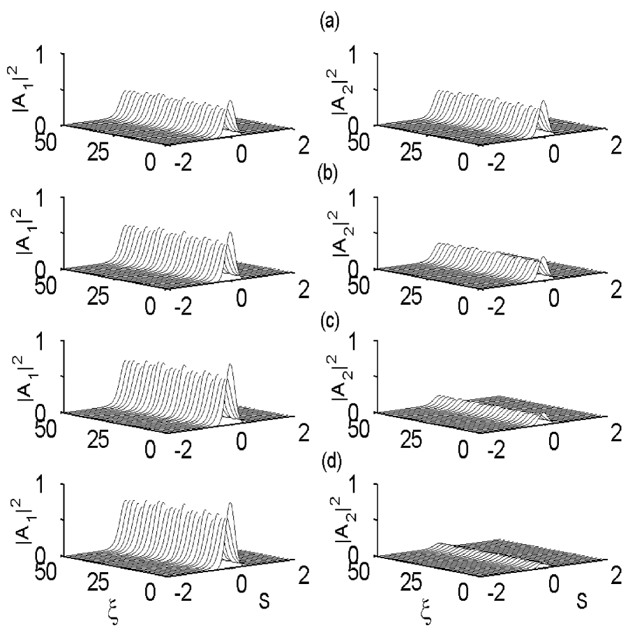
Figure 15: Stable propagation of composite solitons as obtained by direct numerical simulation. $Cr^{2}=4$, $r=1/5$. (a) $P_{1}=0.5,P_{2}=0.5,$ (b) $P_{1}=0.6666,P_{2}=0.3333,$ (c) $P_{1}=0.8333,P_{2}=0.1666$, and (d) $P_{1}=0.909,P_{2}=0.909$ . Left panel $|A_{1}|^{2}$ and right panel $|A_{2}|^{2}$.

To verify the predictions of foregoing analysis, it is essential to perform numerical simulation. Equation (86) has been solved numerically using the split step Fourier beam propagation method  [3]. To begin with, we look for behavior of the soliton at low power. From figure 12(b), we choose $Cr^{2}=4$ and $r=1/5$ and select different points from the curve leveled with this value. Chosen points have following values of $P_{1}$ and $P_{2}$, particularly, (i)$P_{1}=0.5,P_{2}=0.5$, (ii)$P_{1}=0.6666,P_{2}=0.3333$, (iii)$P_{1}=0.8333,P_{2}=0.1666$ and (iv)$P_{1}=0.909,P_{2}=0.0909$. It must be emphasized that each point corresponds to a stationary composite soliton, a paraxial theory prediction. With these parameter values, we launch two Gaussian optical beams $A_{1}=\sqrt{P_{1}}\exp\left(-\frac{s^{2}}{2r^{2}}\right)$ and $A_{2}=\sqrt{P_{2}}\exp\left(-\frac{-s^{2}}{2r^{2}}\right)$ in (86). Both Gaussian beams acquire solitonic shape asymptotically without major modification within very small distance and then they propagate almost as a stationary composite soliton.The behavior of two Gaussian spatial solitons corresponding to each of these points has been depicted in figure (15).

Insert Figure (15) here

It is evident from these figures that a soliton with large power can trap another soliton whose power is much lower and both can propagate as a stationary bound state. At this stage it would be appropriate to cite one practical example. Consider a $BaTiO_{3}$ crystal at a wavelength $\lambda_{0}=0.5\mu m$ with following crystal parameters [64]: $n_{e}=2.365$, $r_{33}=80\times 10^{-12}m/V,$ $E_{p}=10^{5}V/m$. We take arbitrary spatial scale $x_{0}=40\mu m$ and $E_{o}=5.8\times 10^{4}$ V/m. With these values, we find, $\beta=18.4,\ \alpha=31.58$  and $C=2(\alpha+\beta)=99.96$. For $Cr^{2}=4,r\approx 0.20$, thus, in natural unit the intensity FWHM ( i.e.,$1.665r$) of two components is found to be $13.32\mu m$ . An important point to note is that the present investigation is also valid for $LiNbO_{3}$. The $LiNbO_{3}$ parameters could be taken as $n_{e}=2.2,r_{33}=30\times 10^{-12}$m/V and $|E_{p}|=4\times 10^{6}$ V/m. However, it should be pointed out that, while $E_{p}$ could be either positive or negative for $BaTiO_{3}$, depending on the polarization of light, the experimental results show that $E_{p}$ is always negative for $LiNbO_{3}$. Therefore, with proper choice of the value of $E_{o},\ C=2(\alpha+\beta)$ can be made positive, and hence bright-bright coupled soliton pairs is also observable in $LiNbO_{3}$.

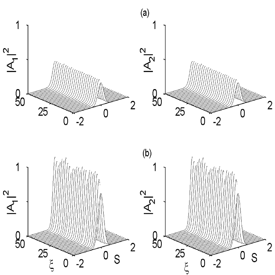
Figure 16: Propagation of bistable composite solitons. Peak power and width of these solitons have been chosen from point A and B of figure (14) which corresponds to $Cr^{2}=4$. Upper panel corresponds to point A and lower panel corresponds to point B. Solitons of both upper and lower panels have same width i.e., each component has spatial width $r=0.290$. Peak power of each component in the upper panel $P=0.321$. Peak power of each component in the lower panel $P=0.779$.

We now proceed to obtain bistable composite solitons numerically. From figure (14) we choose two points A and B, each corresponds to one pair of composite soliton. These two points have equal values of $Cr^{2}(=4.2)$ but two different values of soliton peak power $P$. We have taken $C=50$, hence, $r=0.290$ for both A and B. Peak power P for points A and B are $0.321$ and $0.779$, respectively. Numerically obtained dynamic evolution of a pair of composite bistable solitons corresponding to above values has been demonstrated in figure (16).

Insert Figure (16) here

In the figure, the upper panel represents one composite soliton while the lower panel represents another. From figure, it is evident that both components of the composite in the upper panel remain absolutely stationary as they propagate, an example where paraxial theory prediction complies with high accuracy. However, in the lower panel, both components of the composite propagate as stable self trapped mode though they keep on gentle breathing. Hence, in this case, though prediction of paraxial approximation is not very accurate, yet it is able to capture the overall features broadly. Finally, we have found that bright-bright pairs are stable against small perturbation in peak amplitude and spatial width. Both paraxial theory and numerical simulation show that identified composite solitons are stable.

9.3 Incoherently Coupled Solitons Due to Two-Photon Photorefractive Phenomenon

To investigate coupled solitons in two-photon photorefractive media, the required optical configuration is very similar to the one discussed in sec 8.1. The only difference between this case and the earlier one is that, in the present case there are two incoherent soliton forming beams whose polarization and frequencies are same, whereas in the former case there is only one soliton forming beam. As usual, the optical fields are expressed in the form $\overrightarrow{E_{1}}=\overrightarrow{x}\Phi_{1}(x,z)\exp(ikz)$ and $\overrightarrow{E_{2}}=\overrightarrow{x}\Phi_{2}(x,z)exp(ikz)$, where $\Phi_{1}$ and $\Phi_{2}$ are slowly varying envelopes of two optical fields, respectively. The coupled Schrödinger equations for the normalized slowly varying envelopes of two optical fields can be described as

$$i\frac{\partial U}{\partial\xi}+\frac{1}{2}\frac{\partial^{2}U}{\partial s^{2}}-g\beta\frac{(1+\rho)(1+\sigma+|U|^{2}+|V|^{2})U}{(1+\sigma+\rho)(1+|U|^{2}+|V|^{2})}-\alpha\frac{\eta(g\rho-|U|^{2}-|V|^{2})(1+\sigma+|U|^{2}+|V|^{2})U}{(1+|U|^{2}+|V|^{2})}=0,$$ (98)

and

$$i\frac{\partial V}{\partial\xi}+\frac{1}{2}\frac{\partial^{2}V}{\partial s^{2}}-g\beta\frac{(1+\rho)(1+\sigma+|U|^{2}+|V|^{2})V}{(1+\sigma+\rho)(1+|U|^{2}+|V|^{2})}-\alpha\frac{\eta(g\rho-|U|^{2}-|V|^{2})(1+\sigma+|U|^{2}+|V|^{2})V}{(1+|U|^{2}+|V|^{2})}=0,$$ (99)

where $U=\sqrt{\frac{n_{e}}{2\eta_{0}I_{2d}}}\Phi_{1}$, $V=\sqrt{\frac{n_{e}}{2\eta_{0}I_{2d}}}\Phi_{2}$; parameters $\rho,\ \xi,\ s,\ \beta,\ \alpha,\ \eta,\ \sigma$ have been defined earlier.

Incoherently coupled solitons in two-photon photorefractive media have recently received tremendous attention, since, the dynamics of these solitons can be controlled by a separate gating beam [137, 138, 139, 140, 141, 142, 143, 144, 145, 146, 147, 148, 149, 150, 151, 152]. Properties of these solitons can be investigated using equations (98) and (99).In next few sections we will present a brief description of these solitons.

9.3.1 Incoherently Coupled Two-Photon Photovoltaic solitons Under Open Circuit Condition

In this section, we discuss the existence and nonlinear dynamics of two-component incoherently coupled composite solitons in two-photon photorefractive materials under open circuit condition. In the steady state regime, these incoherently coupled solitons can propagate in bright-dark, bright-bright and dark-dark configurations. These photovoltaic soliton families can be established provided that the carrier beams share same polarization and wavelength, and numerical simulations show that these solitons are stable for small perturbation on amplitude. For photovoltaic solitons under open circuit configuration, $g=0$ and $\beta=0$, hence, relevant Schrödinger equations are

$$i\frac{\partial U}{\partial\xi}+\frac{1}{2}\frac{\partial^{2}U}{\partial s^{2}}+\eta\alpha\frac{(|U|^{2}+|V|^{2})(1+\sigma+|U|^{2}+|V|^{2})U}{(1+|U|^{2}+|V|^{2})}=0,$$ (100)

$$i\frac{\partial V}{\partial\xi}+\frac{1}{2}\frac{\partial^{2}V}{\partial s^{2}}+\eta\alpha\frac{(|U|^{2}+|V|^{2})(1+\sigma+|U|^{2}+|V|^{2})V}{(1+|U|^{2}+|V|^{2})}=0.$$ (101)

9.3.1.1 Bright-dark solitons

We first discuss the properties of photovoltaic bright-dark soliton pairs. To obtain the solution for a bright-dark soliton pair, the normalized envelopes $U$ and $V$ are expressed as

$$U=p^{1/2}f(s)exp(i\mu\xi),$$ (102)

$$V=\rho^{1/2}g(s)exp(i\nu\xi).$$ (103)

In above expressions, $f(s)$ and $g(s)$ are real functions, which correspond to the bright and dark profile, respectively. These real functions are bounded i.e., $0\leq f(s)\leq 1$ and $0\leq g(s)\leq 1$. Also, $p$ and $\rho$ respectively represents the ratio of solitons maximum intensity to the dark irradiance $I_{2d}$. Inserting expressions (102) and (103) in equations (100) and (101), we obtain

$$\frac{d^{2}f}{ds^{2}}-2(\mu-\alpha\eta\sigma)f+2\alpha\eta(pf^{2}+\rho g^{2})f-\frac{2\alpha\eta\sigma f}{1+pf^{2}+\rho g^{2}}=0,$$ (104)

$$\frac{d^{2}g}{ds^{2}}-2(\nu-\alpha\eta\sigma)g+2\alpha\eta(pf^{2}+\rho g^{2})g-\frac{2\alpha\eta\sigma g}{1+pf^{2}+\rho g^{2}}=0.$$ (105)

We look for a particular solution which satisfies the condition $f^{2}+g^{2}=1$. Nonlinear propagation constants $\mu$ and $\nu$ can be determined using appropriate boundary conditions. The value of these turn out to be

$$\mu=\alpha\eta\sigma\left[1-\frac{\log(1+\Delta)}{\Delta(1+\rho)}\right]+\frac{\alpha\eta(p+\rho)}{2},$$ (106)

and

$$\nu=\alpha\eta\rho\left[1+\frac{\sigma}{1+\rho}\right],$$ (107)

where $\Delta=\left(\frac{p-\rho}{1+\rho}\right)$. At this stage a comment on the sign of $\alpha$ for the existence of bright-dark solitons is desirable. In order to do that we integrate equation(104) to obtain

$$s=\pm\frac{1}{(-\alpha\eta)^{1/2}}\int_{1}^{f}\left[\frac{2\sigma}{\Delta(1+\rho)}(f^{2}\log(1+\Delta)-\log(1+\Delta f^{2}))+(p-\rho)f^{2}(f^{2}-1)\right]^{1/2}df.$$ (108)

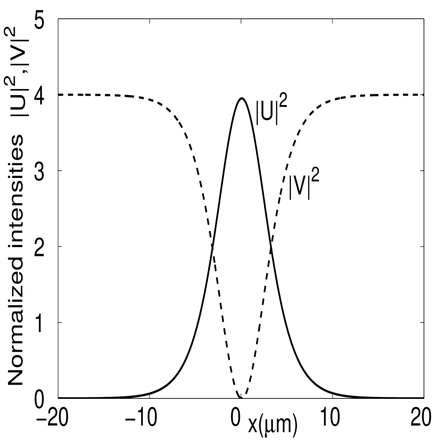
Figure 17: Soliton components $|U|^{2}$ and $|V|^{2}$ of the bright-dark soliton pair for $\rho=4,p=3.95$, $\sigma=10^{6}$ and $\alpha=-22.2$. Gating beam intensity $I_{1}=10^{6}W/m^{2}$ and calculated value of $\Delta=-0.01$.

The sign of the integrand within the third bracket depends on the parameters $p,\ \rho$ and $\sigma$. For a given set of experimentally relevant values of the aforesaid parameters, for example, when $p=3.95,\rho=4.0$ and $\sigma=10^{6}$, the integrand within the third bracket is positive. Thus, for above set of parameters the existence of dark-bright solitons requires $\alpha<0$ i.e., $E_{p}<0$. For illustration, we consider a $LiNbO_{3}$ crystal with the following parameters $n_{e}=2.2$ and $r_{33}=30\times 10^{-12}$ $mV^{-1}$at wavelength $\lambda_{0}$. Other parameters are taken as $E_{p}=-4\times 10^{6}$ $Vm^{-1}$, $s_{1}=3\times 10^{-4}m^{2}W^{-1}s^{-1}$, $\gamma_{1}=3.3\times 10^{-17}m^{3}s^{-1},\ N_{A}=10^{22}m^{-3},\ \beta_{1}=0.5s^{-1},\ \beta_{2}=0.5s^{-1}$ and $s_{2}=3\times 10^{-4}m^{2}W^{-1}s^{-1}$. The gating beam intensity $I_{1}=10^{6}W/m^{2}$, the scaling parameter $x_{0}=0.5\mu m$, therefore, $\alpha\approx-22.2$ and $\eta=1.67\times 10^{-4}$. The value of $\sigma$ can be controlled by modulating the dark irradiance artificially using incoherent illumination [93] and for the present investigation we take $\sigma=10^{6}$ and $\rho=4$. A typical bright-dark pair has been depicted in figure (17).

Insert Figure (17) here

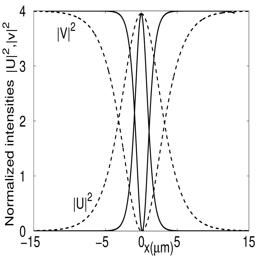
Figure 18: Soliton components $|U|^{2}$ and $|V|^{2}$ of the bright-dark soliton pair for two different values of the gating beam intensity $I_{1}$. Values of different parameters are $\rho=4,p=3.95,\sigma=10^{6}$ and $\alpha=-22.2$. Solid line for $I_{1}=10^{5}W/m^{2}$, dashed line for $I_{1}=10^{6}W/m^{2}$.

In order to examine the influence of the gating beam on these solitons, we have numerically computed profiles of these solitons at two different values of the gating beam intensities. This has been depicted in figure (18). With the change in $I_{1}$ , the width of each component changes.

Insert Figure (18) here

9.3.1.2 Bright-bright solitons

We now investigate two component bright-bright solitons. In this case, intensities of both soliton forming optical beams vanish at infinity i.e., as $s\rightarrow\pm\infty,\ I_{2\infty}=0$. The soliton solution is now expressed in terms of normalized envelopes $U$ and $V$ as

$$U=p^{1/2}y(s)cos\theta\exp(i\mu\xi),$$ (109)

$$V=p^{1/2}y(s)sin\theta\exp(i\mu\xi),$$ (110)

where $p$ represents the ratio of the peak intensity to the dark irradiance $I_{2d},\ \mu$ is the nonlinear shift of the propagation constant, $y(s)$ is the normalized real function which is bounded as $0\leq y(s)\leq 1$ , $\theta$ is an arbitrary projection angle which describes relative strength of two components of the composite. Substitution of expressions (109) and (110) in either of equations (100) or (101) yields the following differential equation,

$$\frac{d^{2}y}{ds^{2}}=2(\mu-\alpha\eta\sigma)y-2\alpha\eta py^{3}+\frac{2\alpha\eta\sigma y}{1+py^{2}}=0.$$ (111)

Integrating above equation once, we obtain,

$$\left(\frac{dy}{ds}\right)^{2}=2(\mu-\alpha\eta\sigma)(y^{2}-1)-\alpha\eta p(y^{4}-1)+\frac{2\alpha\eta\sigma}{p}\log\left(\frac{1+py^{2}}{1+p}\right).$$ (112)

Making use of the boundary conditions $y(\pm\infty)=0$ and $\dot{y}(\pm\infty)=0$, we can easily obtain $\mu$ as

$$\mu=\alpha\eta\sigma\left[1-\frac{\log(1+p)}{p}\right]+\frac{\alpha\eta p}{2}.$$ (113)

Inserting equation (113) in (112) we get,

$$\left(\frac{dy}{ds}\right)^{2}=\alpha\{\frac{2\eta\sigma}{p}[\log(1+py^{2})-y^{2}\log(1+p)]+\eta py^{2}(1-y^{2})\}.$$ (114)

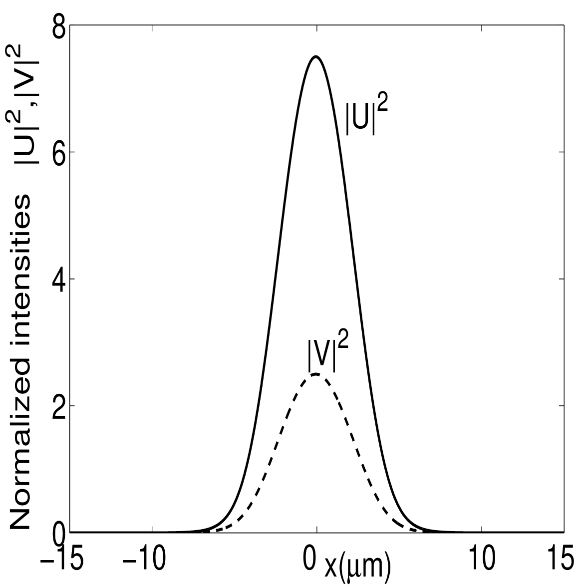
Figure 19: Soliton components $|U|^{2}$ and $|V|^{2}$ of the bright-bright soliton pair when $p=10$ and $\theta=30^{0}$.

From equation (114) we can easily show that the quantity within the curly bracket in the right hand side is positive for all the values of $y^{2}(s)$ i.e., $0\leq y(s)\leq 1$, therefore, we easily conclude that $\alpha>0$ for bright-bright solitons. In order to investigate bright-bright soliton pair, we take a Cu:KNSBN crystal, whose parameters at $\lambda_{0}=0.5\mu m$ are taken as $n_{e}=2.2$, $r_{33}=200\times 10^{-12}mV^{-1}$ and $E_{p}=2.8\times 10^{6}Vm^{-1}$. The scaling parameter $x_{0}=10\mu m$, $p=10$ and $\theta=30^{0}$. Other parameters for the bright-bright soliton configuration are: $\alpha=22.2$, $\eta=1.5\times 10^{-4}$ and $\sigma=10^{4}$. Figure (19) depicts the normalized intensity profile of the photovoltaic bright-bright soliton pair.

Insert Figure (19) here

9.3.1.3 Dark-dark solitons

Properties of dark-dark soliton pairs can be analyzed following similar procedure as elucidated in previous sections. In the case of dark type profiles, there is a constant intensity background i.e., $I_{2\infty}\neq 0$, therefore we express normalized envelopes $U$ and $V$as

$$U=\rho^{1/2}y(s)cos\theta\exp(i\mu\xi),$$ (115)

$$V=\rho^{1/2}y(s)sin\theta\exp(i\mu\xi),$$ (116)

where, $\rho=I_{2\infty}/I_{2d}$ and $0\leq y(s)\leq 1$. As usual $\mu$ is the nonlinear shift of the propagation constant, and $\theta$ is the projection angle. Furthermore, inserting equations (115) and (116) in either of equation (100) or (101), we obtain

$$\frac{d^{2}y}{ds^{2}}=2(\mu-\alpha\eta\sigma)y-2\alpha\eta\rho y^{3}+\frac{2\alpha\eta\sigma y}{1+\rho y^{2}}.$$ (117)

Above equation can be solved easily adopting numerical procedure after evaluationg the nonlinear propagation constant $\mu$. An important point to note is that dark-dark soliton pairs require $\alpha<0$. For illustration, we take a $LiNbO_{3}$ crystal with $n_{e}=2.2$ and $r_{33}=30\times 10^{-12}mV^{-1}$ at wavelength $\lambda_{0}=0.5\mu m$. Other parameters are $E_{p}=-4\times 10^{6}Vm^{-1}$, $s_{1}=3\times 10^{-4}m^{2}W^{-1}s^{-1}$, $\gamma_{1}=3.3\times 10^{-17}m^{3}s^{-1}$, $N_{A}=10^{22}m^{-3}$, $\beta_{1}=0.5s^{-1},\beta_{2}=0.5s^{-1}$ and $s_{2}=3\times 10^{-4}m^{2}W^{-1}s^{-1}$. The gating beam intensity $I_{1}$is taken to be $10^{6}W/m^{2}$ and the scaling parameter $x_{0}=0.5\mu m$. Therefore, $\alpha\approx-22.2$, $\eta=1.67\times 10^{-4}$. We take $\sigma=10^{6}$ and $\rho=4$. A dark-dark soliton pair is depicted in figure (20). Numerical simulation confirms that these solitons are robust, do not break up or disintegrate if small perturbation in amplitude is introduced.

Insert Figure (20) here

10 Conclusion

We have presented a brief review of the recent developments in the field of optical spatial solitons in photorefractive media. In relatively short time this topic has achieved tremendous success in theory as well as in experiments. We have considered fundamental properties of three types of solitons, particularly, screening, photovoltaic and screening photovoltaic solitons and described different methods to investigate them. For each type of soliton, three different configurations i.e., bright, dark and gray varieties have been considered. Self bending of these solitons due to diffusion and effect of higher order diffusion on self bending phenomenon are also highlighted. Besides single photon photorefractive phenomenon, lately the two-photon photorefractive phenomenon has become a topic of intense research since the PR effect can be controlled with a separate gating beam. Mechanisms of formation of PR solitons due to single photon as well as two-photon photorefractive processes have been discussed. Interaction of solitons is an extremely important topic which could be exploited to fabricate all optical switching devices. We have discussed important properties associated with interaction of these solitons. Vector solitons, particularly, incoherently coupled solitons due to single photon and two-photon photorefractive phenomena have been highlighted. Existence of some missing solitons pointed out. Several properties discovered so far for these solitons are universal and applicable to other branches of solitons.

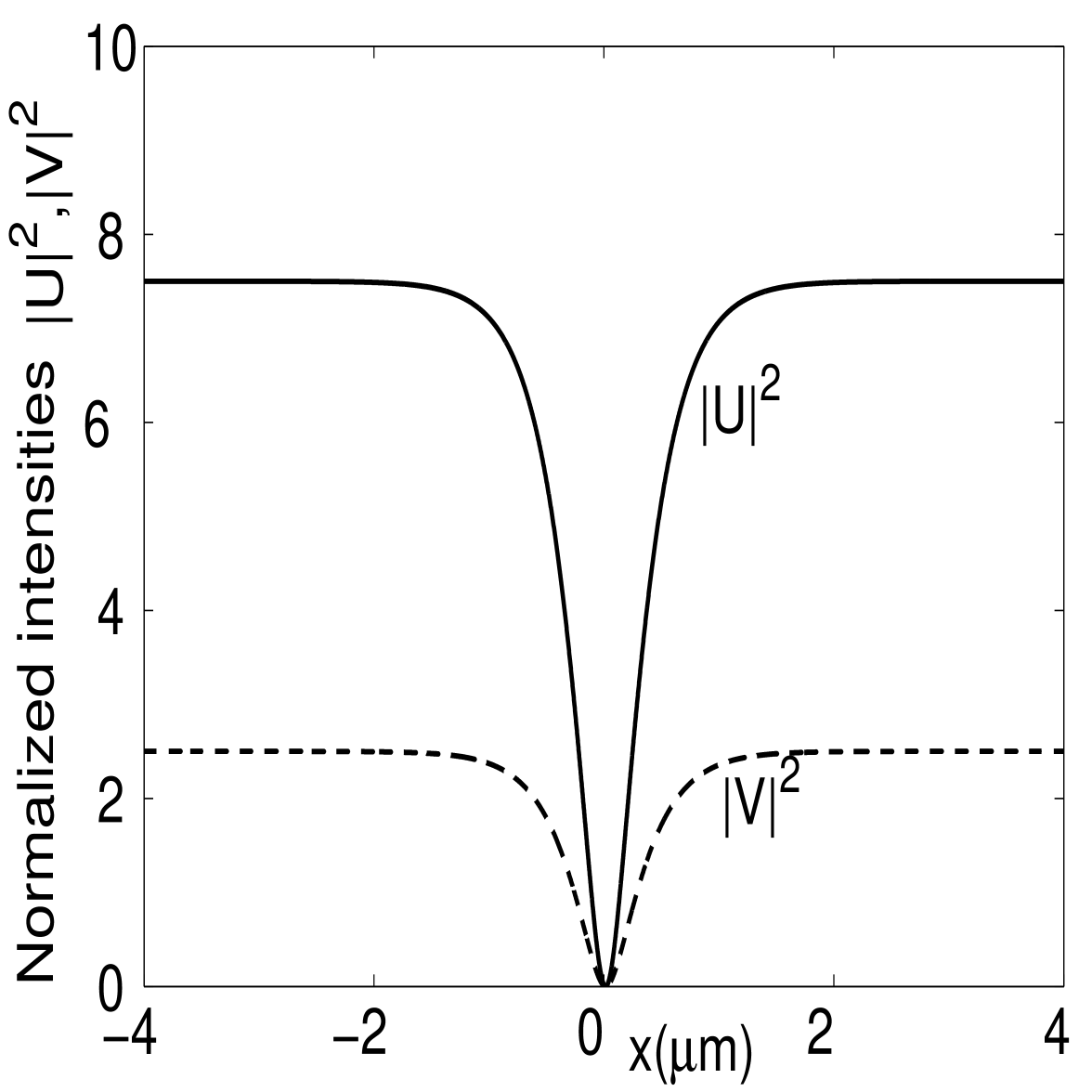
Figure 20: Soliton components $|U|^{2}$ and $|V|^{2}$ of the dark-dark soliton pair when and $\rho=10$ and $\theta=30^{0}$.

References

- Hasegawa et al. [1973] A. Hasegawa and F. Tappert, Appl. Phys. Letts. 23(1973)142-145.
- Mollenaue et al. [1980] L. F. Mollenaue, R. H. Stolen and J. P. Gordon, Phys. Rev. Letts. 45(1980)1095.
- Agrawal et al. [1989] G. P. Agrawal, Academic Press, New York (1989).
- Zabusky et al. [1965] N.J.Zabusky and M.D. Kruskal, Phys. Rev. Letts. 15(1965)240.
- Kivshar et al. [2001] Y.S. Kivshar and A. A. Sukhorukov, in Spatial Solitons, S. Trillo and W. Toruellas, Eds.( Springer, New York, 2001) pp 211-246.
- Akhmediev et al. [1997] N. N. Akhmediev and A. Ankiewicz, Solitons: Nonlinear Pulses and Beams (Chapman and Hall, London 1997, Chapter 3).
- Malomed et al. [2005] B. A. Malomed, D. Mihalache, F. Wise and L. Torner; J. Opt. B: Quantum Semiclass. Opt. 7(2005)R53-R72.
- Kivshar et al. [2003] Y. S. Kivshar and G. P. Agrawal, Optical Solitons: From Fibers to Photonic Crystals, Academic Press, San Diogo, California, 2003.
- Mihalache et al. [2008] D. Mihalache, D. Mazilu, F. Lederer, H. Leblond and B. A. Malomed; Physical Review A 77(2008)033817.
- Crosignani et al. [1993] B. Crosignani, M. Segev, D. Ergin, P. Di Porto, A. Yariv and G. Salamo, J. Opt. Soc. Am B 10( 1993)446-453.
- L et al. [2008] X. L, Hong-Wu Zhu, Zhen-Zhi Yao, Xiang-Hua Meng, Cheng Zhang, Chun-Yi Zhang, B. Tian; Annals of Physics 323, (2008)1947-1955.
- Tian et al. [2011] B.Tian and Jixiong Pu; Optics Letters 36(2011)2014-2016
- L et al. [2008] X. L, B. Tian, Tao Xu, Ke-Jie Cai, Wen-Jun Liu; Annals of Physics 323(2008)2554-2565.
- Liu et al. [2010] W. J. Liu, B. Tian, Tao Xu, Kun Sun, Yan Jiang; Annals of Physics 325(2010)1633-1643.
- Tienman et al. [2008] M. Tiemann, J. Petter, T. Tschudi, Optics Commun. 281(2008)175-180.
- Tienman et al. [2009] M. Tiemann, T. Halfmann, T. Tschudi, Opt. Commun. 282(2009)3612-3619.
- Anjan Biswas et al. [2006 ] Anjan Biswas and Swapan Konar; Non-Kerr Law Optical Solitons, CRC Press, New York (2006).
- Duree et al. [1993] G. C. Duree, J. L. Sultz, G. J. Salamo, M. Segev, A. Yariv, B.Crosignani, P. Di Porto, E. J. Sharp, R. R. Neurgaonkar, Phys.Rev. Letts. 71(1993)533-536.
- Karamzin et al. [1975] Y. N. Karamzin, A. P. Sukhorukov, Soviet Physics JETP 41(1975)414.
- Sukhorukov et al. [2000] A. A. Sukhorukov, Phys. Rev. E 61(2000)4530.
- Mihalache et al. [1997] D. Mihalache, D. Mazilu, L. C. Crasovan and L.Toner, Optics Commun. 137(1997)113.
- Darmanyan et al. [1998] S. Darmanyan, A. Kobyakov and F. Lederer, Phys. Rev. E 57(1998)2344.
- Sirtori et al. [1992] C. Sirtori, F. Capsso, D.L. Sivco and A.Y. Cho, Phys. Rev. Letts. 68(1992)1010.
- Schmidt et al. [1996] H. Schmidt and A. Imamoglu, Opt. Letts. 21(1996)1936.
- Yang et al. [2009] X. Yang, S. Li, C. Zhang and H. Wang, J. Opt Soc. Am. B 26(2009)1423.
- Doyeol et al. [1987] A. Doyeol and S.L. Chuan, IEEE J. Quntum Electron. QE-23(1987)2196.
- Rosencher et al. [1991] E. Rosencher and P. Bois, Phys. Rev. B 44(1991)11315.
- Chauvet et al. [2001] M.Chauvet, S.Chauvin, H.Maillotte, Opt. Letts. 26(2001)1344.
- Bosshard et al. [1994] C. Bosshard, P. V. Mamyshev, G. I. Stageman, Opt. Letts. 19(1994)90.
- Chauvet et al. [1997 ] M.Chauvet, S.A.Hawkins, G. Salamo, M. Segev, F. D. Bliss, G. Bryant, Appl. Phys. Letts. 70(1997)2499.
- Fazio et al. [2004] E. Fazio, F. Renzi, R. Rinaldi, M. Bertolotti, M. Chauvet, W. Ramadan, A. Petris, and V. I. Vlad, Appl. Phys. Letts. 85(2004)2193-2195.
- Kuroda et al. [2002] K. Kuroda, in Progress in Photorefractive Nonlinear Optics, Eds Kazuo Kuroda, Taylor and Francis New York (2002).
- Chen et al. [1968 ] F. S. Chen, J. T. LaMacchia and D. B.Fraser, Appl. Phys. Letts. 13(1968)223.
- Yeh et al. [1993 ] P. Yeh; Introduction to photorefractive nonlinear optics, Wiley 1993.
- Gunter et al. [2006 ] P. Gunter and J.P.Huignard (Eds), Photorefractive Materials and Their Applications, Springer (2006).
- Ashkin et al. [1996] A. A.Ashkin, G. D. Boyd, J. M. Dziedzic, R.G. Smith, A. A. Ballmann, H. J. Levinstin and K. Nassau, Appl. Phys. Letts. 9(1966)72.
- Meerhotz et al. [1994] K. Meerhotz, B. L. Volodin, S. B. Kippelen and N. Peyghambarian, Nature 371(1994)497 .
- Moerner et al. [1994] W. E. Moerner and S. M. Silence, Chem. Rev. 94(1994)127.
- Shih et al. [1999] M.F.Shih and F.W. Sheu, Optics Letts. 24(1999)1853.
- Sheu et al. [2001] F. W.Sheu and M. F. Shih, J. Opt. Soc. Am. B 18(2001)785.
- Kukhtarev et al. [1979] N. V. Kukhtarev, V.B. Markov, S. G. Odulov, M. S. Soskin and V.L. Vinetskii, Ferroelectrics 22(1979) 949.
- DelRe et al. [2001] E. DelRe, A. Ciattoni and A. J. Agranat,Opt. Letts. 260(2001)908-910.
- Saffman et al. [1998] M. Saffman and A. A. Zozulya, Opt.Letts. 23(1998)1579.
- Liu et al. [1999] J. S. Liu and K. Q. Lu, J. Opt. Soc. Am B 16(1999)550-555.
- Carvalho et al. [1996] M. I. Carvalho, S. R. Singh, D. N. Christodoulides, Opt.Commun. 124(1996)642.
- Christodoulides et al. [1995] D. N. Christodoulides and M. I. Carvalho, J. Opt. Soc.Am B 12(1995)1628-1633.
- Segev et al. [1994] M. Segev, G. C. Valley, B. Crosignani, P. Di Porto, and A. Yariv, Phys. Rev. Letts. 73(1994)3211.
- Shih et al. [1995] M.F.Shih, M. Segev, G.C. Valley, G. Salamo, B. Crosignani,P. Di Porto, Electron. Lett. 31(1995)826.
- Chen et al. [1996] Z. Chen, M. Mitchell, M.F. Shih, M Segev, M H.Garrett, G. C. Valley, Opt. Letts. 21(1996)629.
- Iturbe-Castillo et al. [1994] M. D. Iturbe-Castillo, P. A. Aguilar, J. J.Sánchez-Mondragón, S. Stepanov, V. Vysloukh, Appl. Phys. Letts. 64(1994)408
- Garca-Quirino et al. [1997] G. S. Garca-Quirino, M. D. Iturbe-Castillo, V. A. Vysloukh, J.J. Sánchez-Mondragón, S. I. Stepanov, G.Lugo-Martnez and G. E. Torres-Cisneros, Opt. Letts. 22(1997)154
- Mamaev et al. [1996] A.V. Mamaev, M. Saffman and A. A. Zozulya, Europhys. Letts. 35(1996)25
- Mamaev et al. [1996] A. V. Mamaev and M. Saffman, Phys. Rev. Letts. 76(1996)2262
- Mamaev et al. [1997] A. V. Mamaev, A. A. Zozulya, V. K. Mezentsev, D. Z. Anderson and M. Saffman, Phys. Rev. A 56(1997)R1110-R1113.
- Krolikowski et al. [1998] W. Krolikowski, M. Saffman, B. Luther-Davies, and C.Denz, Phys. Rev. Letts. 80(1998)3240.
- Konar et al. [2011] S.Konar, Phys. Express 1(2011)139.
- Valley et al. [1994] G. C. Valley, M. Segev, B. Crosignani, A. Yariv, M. M. Fejer and M. C. Bashaw, Phys. Rev. A 50(1994)R4457 .
- Taya et al. [1995] M. Taya, M. C. Bashaw, M. M. Fejer, M. Segev and G.C. Valley, Phys. Rev. A 52(1995)3095.
- Chen et al. [1997] Z. Chen, M. Segev, D. W. Wilson, R. E.Muller and P. D. Maker, Phys. Rev. Letts. 78(1997)2948.
- Liu et al. [1999] J.S.Liu and K.Q. Lu, J.Opt. Soc. Am B 16,(1999)550.
- Segev et al. [1997] M. Segev, G. C. Valey, M.C. Bashaw, M. Taya and M. M. Fejer; J. Opt. Soc. Am. B 14,(1997) 1772.
- She et al. [1999] W. L. She, K. K. Lee and W. K. Lee, Phys. Rev. Letts. 83(1999)3182 .
- Couton et al. [2004] G. Couton, H.Maillotte, M. Chauvet, J. Opt. B: Quantum Semiclass. Opt. 6(2004)S223.
- Konar et al. [2007] S. Konar, S. Jana, S. Shwetanshumala, Opt. Commun. 273(2007)324.
- Vakhitiov et al. [1973] N. G.Vakhitiov and A. A. Kolokolov, Sov. Radio Phys. 16(1973) 783.
- DeAngelis et al. [1994] C. DeAngelis, IEEE J. QE 30,(1994) 818.
- Kumar et al. [1996] A.Kumar, T. Kurz and W. Lauterborn, Phys. Rev. E 53(1996)1166.
- Kaplan et al. [1985] A. E. Kaplan, Phys. Rev. Letts. 55(1985) 1291.
- Hasegawa et al. [1973] A. Hasegawa and F. Tappert, Appl. Phys. Letts. 23(1973)171.
- Krolikowski et al. [1996] W. Krolikowski, N. Akhmediev, B. Luther Davies, M. C. Golomb, Phys. Rev. E 54, (1996)5761-5765.
- Carvalho et al. [1995] M. I. Carvalho, S. R. Singh and D. N. Christodoulides, Opt. Commun. 120(1995)311.
- Carvalho et al. [2007] M. I.Carvalho, M. Facco and D. N. Christodoulides, Phys Rev E 76(2007)016602.
- Zhan et al. [2010] K. Zhan, C.F. Hou, Yanwei Du, Opt. Commun. 283(2010)138-141.
- Zhang et al. [2008] G.Zhang, J.S.Liu, W. Cheng, Z.Huilan and S.Liu, Optik 119(2008) 3003-3008.
- Liu et al. [2007] S.Liu, J.S. Liu, H. Zhang, G.Zhang, W. Cheng, J.Modern Optics 54(2007)2795-2805.
- Petter et al. [1999] J. Petter, C. Weilnau, C. Denz, A. Stepken, F. Kaiser, Optics Commun. 170(1999)291.
- Zhang et al. [2009] G. Zhang, Y. Han, L.Tao, A. Zheng, Q. Du, Optics and Laser Technology 41 (2009)596-600.
- Liu et al. [2001] J.S. Liu, D. Zhang, Z Hao, J. Modern Opt. 48(2001)1803-1810.
- Zhang et al. [2006] G.Zhang, J.S.Liu, S.Liu, H.Zhang and W. Cheng, J. Opt. A: Pure Appl. Opt. 8(2006)442-449.
- Liu et al. [2003] J.S.Liu and Z. Hao, Chinese Physics 12 (2003)1124.
- Liu et al. [2002] J.S. Liu and Z. Hao, J. Opt. Soc. Am B 19(2002)513.
- Jiang et al. [2009] Q. C.Jiang, Y. L.Su, X. M.Ji, Chinese J. Quantum Electron. 26(2009)619-623.
- Kodama et al. [1987] Y. Kodama and A. Hasegawa, IEEE J. QE 223(1987)510.
- Blow et al. [1988] K. J. Blow, N. J. Doran and D. Wood, J.Opt. Soc. Am B 5(1988)1301.
- Sodha et al. [2008] M. S. Sodha, S. K. Agrawal and A. Sharma, J. Plasma Physics 74(2008)65-77.
- Konar et al. [1994] S. Konar, A. Sengupta, J.Opt. Soc. Am. B 11 (1994) 1644.
- Sturman et al. [1992] B. I. Sturman and V. M.Fridkin, The photovoltaic and photorefractive effects in non-centrosymmetric materials ( Philadelphia, Gordon and Breach 1992).
- Zhang et al. [2007] G. Zhang, J.S. Liu, H. Zhang, C. Wang, S.Liu, Optik 118 (2007)440-444.
- Liu et al. [2002] J.S. Liu and Z. Hao, Chinese Physics 11(2002)254-259.
-
Ramadan et al. [2003]
W. Ramadan, E.Fazio, A.Mascioletti, F.Inam, R.Rinaldi,A.Bosco, V.I.Vlad, A.Petris and M.Bertolotti, J. Opt. A: Pure Appl.
Opt. 5(2003)S432.
- Castro-Camus et al. [2003 ] E. Castro-Camus and L.F.Magana, Opt. Letts. 28(2003)1129.
- Hou et al. [2005 ] C. F. Hou, Y. B. Pei, Z. X. Zhou and X. D.Sun, Phys. Rev. A 71 (2005)053817.
- Hou et al. [2007 ] C. F. Hou, Y. Zhang, Y. Y. Jiang and Y.B. Pei, Opt. Commun. 273(2007) 544-548.
- Zhang et al. [2009 ] G. Zhang, J.S. Liu, J. Opt. Soc. Am.B 26 (2009)113.
- Konar et al. [2010 ] S.Konar, S. Shekhar and W.P.Hong, Optics and Laser Technology 42(2010) 1294-1300 .
- Zhang et al. [2007 ] Y.Zhang, C.F.Hou and S.X. Dong, Chinese Physics 16 (2007)159.
- Jiang et al. [2010 ] Q. Jiang, Y. Su and X. Ji, Optica Applicata Vol XL. No 2. (2010)481.
- Jiang et al. [2011 ] Q. Jiang, Y. Su and X. Ji, Optics and Laser Technology 43 (2011)91-94.
- Ji et al. [2010 ] X. Ji, Q. Jiang, J. Yao, J.S. Liu, Optics and Laser Technology 42(2010)322-327.
- Jiang et al. [2011 ] Q.Jiang, Y.Su, X. Ji, Optik 122(2011)490-493.
- Su et al. [2010 ] Y. L. Su, Q. C. Jiang, X.M.Ji, Chinese J. of Quantum Electron. 27(2010)331-335.
- Zhang et al. [2010 ] G. Zhang, Y. Cheng, Z. Luo, L. Tao and Q. Du, Optics Commun. 283(2010)335-339.
- Vlad et al. [2006 ] V. I. Vlad, A. Petris, A. Bosco, E. Fazio and M. Bertolotti, J. Opt. A: Pure Appl. Opt. 8 (2006) S477- S482.
- Segev et al. [1995 ] M. Segev, G. C. Valley, S. R. Singh, M.I. Carvalho, D. N. Christodoulides, Opt. Letts. 20(1995)1764.
- Carvalho et al. [1996 ] M. I. Carvalho, S. R. Singh, D. N. Christodoulides. R. I. Joseph, Phys. Rev E 53 (1996)R53.
- Lu et al. [2002] K. Lu, S.Qian, W.Zhao, Y.Zhang, Z. Wu, Optics Commun. 209 (2002)437-444.
- Lu et al. [2004 ] K.Q. Lu, W. Zhao, Y. Yang, C.Sun, X. Bin, Y.Zhang and J. Xu, J. Opt. A: Pure Appl. Opt. 6 (2004)658-665.
- Christodoulides et al. [ 1996] D.N. Christodoulides, S. R. Singh, M. I. Carvalho and M. Segev, Appl. Phys. Letts. 68 (1996)1763.
- Chen et al. [1997 ] Z. Chen, M. Segev, T.H. Coskun, D.N. Christodoulides and Y.S. Kivshar, J. Opt. Soc. Am. B 14 (1997)3066.
- Chen et al. [ 1996] Z. Chen, M. Segev, T. H. Coskun, D. N. Christodoulides, Opt. Lett. 21 (1996)1436-1438.
- Chen et al. [1996 ] Z. Chen, M. Segev, T. H. Coskun, D. N. Christodoulides, Y.S. Kivshar and V. V. Afanasjev, Opt. Letts. 21(1996)1821.
- Hou et al. [2002] C.F. Hou, Y.Jiang, B. Yuan, X. Sun, C. Du, S. Li, Optical Materials 19(2002)377-381.
- Lu et al. [2005] K.Q. Lu, W.Zhao, Y. Yang, G.Chen, J. Xu, Y. Zhang, X. Hou, Optical Materials 27 (2005) 1845-1850.
- Chen et al. [1996] Z. Chen, M. Segev, T. H. Coskun and D. N. Christodoulides, Opt. Letts. 21(1996)1436.
- Zakery et al. [2004] A. Zakery and K.Keshavarz, J. Phys. D: Appl. Phys. 37(2004)3409-3418.
- Zakery et al. [2004] A. Zakery, A. Keshavarz, Optik 115 (2004) 507-511.
- Hou et al. [2002] C.F. Hou, D.C.Guang, Abdurusul, S.Q.Li, Chinese Phys. Letts. 19 (2002)63.
- Hou et al. [2001] C.F. Hou, L. Bin, X.D.Sun , Y.Y. Jiang and X.K.Bin, Chinese Phys. 10 (2001) 310-314.
- Hou et al. [2001] C. Hou, Z.Zhou, B.Yuan and X.Sun, Appl. Phys B 72 (2001)191-194.
- Lu et al. [2001] K.Q. Lu,Y.Zhan, T.Tang and B. Li, Phys Rev E 64(2001)056603.
- Weilnau et al. [2001] C. Weilnau, W. Krolikowski, E. A. Ostrovskaya, M. Ahles, M. Geisser, G. McCarthy, C. Denz, Y. S. Kivshar and B. Luther Davies, Appl. Phys B 72 (2001)723-727.
- Hong et al. [2008] W. P. Hong, J. Korean Physical Society 53 (2008) 3207-3212.
- Hou et al. [2004] C. Hou, Z. Zhou, X. Sun, Opt. Mater. 27 (2004)63.
- Gardner et al. [1967] C.S. Gardner, J.M. Greene, M. D. Kruskal, and R. M. Miura, Phys. Rev. Letts. 19 (1967)1095.
- Ablowitz et al. [1981] M. J. Ablowitz, H. Segur, Solitons and the Inverse Scattering Technique, SIAM, Philadelphia, 1981.
- Akhmanov et al. [1968] S.A. Akhmanov, A.P. Sukhorukov and R.V. Khokhlov, Sov. Phys. USP. 10 (1968)609.
- Akhmanov et al. [1972] S.A. Akhmanov, A.P. Sukhorukov, R.V. Khokhlov, A.T. Arechi, E.D. Shulz Dubois (Eds.), Laser Handbook, Vol. II, North Holland, Amsterdam, 1972, p. 1151.
- Vlasov et al. [1971] S.N.Vlasov, V.A.Petrischev and V.I.Talanov, Sov. Radio Phys. 14(1971)1062.
- Anderson et al. [1983] D. Anderson, Phys. Rev. A 27 (1983)3135.
- Malomed et al. [1997] B.Malomed, D. Anderson, M. Lisak and M. L. Quiroga-Teixeiro and L. Stenflo, Phys. Rev. E 55 (1997)962.
- Mihalache et al. [2010] D. Mihalache, D. Mazilu, V. Skarka, B. A. Malomed,3H. Leblond, N. B. Aleksc, and F. Lederer ; Physical Review A 82 (2010) 023813
- Mihalache et al. [2007] D. Mihalache, D. Mazilu, F. Lederer, H. Leblond, and B. A. Malomed; Physical Review A 75, (2007) 033811 .
- Mihalache et al. [2010] D. Mihalache, D. Mazilu, V. Skarka, B.A.Malomed, H. Leblond, N.B.Aleksc, F. Lederer; Phys. Rev. A 82 (2010)023813.
- Jana et al. [2007] S. Jana and S. Konar, Phys. Letts. A 362, (2007)435-438.
- Anderson et al. [2001] D. Anderson, M. Lisak and A. Berntson, Pramana-journal of Physics 57 (2001)917.
- Zhang et al. [2008] Y. Zhang, C.F. Hou, F.Wang, X.Sun, Optik 119 (2008)700
- Lu et al. [2007] K. Lu, W.Zhao, Y. Yang, Y. Yang, M. Zhang, R. A. Rupp, M. Fally, Y. Zhang and J. Xu, Appl. Phys. B 87(2007)469-473.
- Zhan et al. [2010] K. Zhan, C.F. Hou, H. Tian, S. Pu and Y Du, J Opt. 12 (2010)015203.
- Zhan et al. [2010] K. Zhan,C.F. Hou and Y.Zhang, J. Opt. 12 (2010)035208.
- Zhan et al. [2010] K.Zhan, C.F. Hou, T.Hao, Y.Zhang, Phys. Letts. A 374 (2010)1242.
- Jiang et al. [2010] Q. Jiang, Y. Su, X. Ji, Optics and laser Technology 42 (2010)720-723.
- Konar et al. [2010] S. Konar and N. Asif, Phys. Scr. 81 (2010)015401.
- Asif et al. [2008] N. Asif, S. Shwetanshumala and S. Konar, Phys. Letts. A 372 (2008)735-740.
- Srivastava et al. [2009] S. Srivastava and S.Konar, Optics and Laser Technology 41 (2009)419-423.
- Su et al. [2010] Y. L. Su, Q. C. Jiang and X. M. Ji, Commun. Theor. Phys. 53 (2010)943-946.
- Keshavarz et al. [2009] A. Keshavarz, L. Sadralsadati and M. Hatami, Progress In Electromagnetics Research Symposium Proceedings, Moscow, Russia, August 18-21, pp-1823(2009).
- Ji et al. [2012] Xuanmang Ji, Jinlai Wang, Qichang Jiang and Jinsong Liu; Phys. Scr. 85 (2012) 025403.
- Zhang et al. [2011] Y.Zhang, C.F Hou, K. Zhan, X. Sun, Optik 122 (2011)263-265.
- Ji et al. [2010] S.H.Ji, Laser Technology 34 (2010) 202
- Zhan et al. [2010] K Y Zhan, C F Hou, H Tian, S Z Pu and Y W Du; J. Opt. 12(2010) 015203.
- Su et al. [2011] Y. Su, Q. Jiang, X. Ji and J. Wang, Optics and Lasers in Engineering 49(2011)526 529.
- Zhang et al. [2007] Y. Zhang, C. F. Hou, X. D. Sun, Acta. Phys. Sin 56,(2007)3261.